Efficient Homomorphic Evaluation on Large Intervals
←
→
Page content transcription
If your browser does not render page correctly, please read the page content below
Efficient Homomorphic Evaluation
                        on Large Intervals

              Jung Hee Cheon12 , Wootae Kim1 , and Jai Hyun Park(           )1

    1
        Department of Mathematical Sciences, Seoul National University, South Korea
                       {jhcheon, wo01416, jhyunp}@snu.ac.kr
                           2
                             Crypto Lab Inc., South Korea

          Abstract. Homomorphic encryption (HE) is being widely used for privacy-
          preserving computation. Since HE schemes only support polynomial op-
          erations, it is prevalent to use polynomial approximations of non-polynomial
          functions. We cannot monitor the intermediate values during the homo-
          morphic evaluation; as a consequence, we should utilize polynomial ap-
          proximations with sufficiently large approximation intervals to prevent
          the failure of the evaluation. However, the large approximation inter-
          val potentially accompanies computational overheads, and it is a serious
          bottleneck of HE application on real-world data.
          In this work, we introduce domain extension polynomials (DEPs) that
          extend the domain interval of functions by a factor of k while preserving
          the feature of the original function on its original domain interval. By
          repeatedly iterating the domain-extension process with DEPs, we can
          extend with O(log K) operations the domain of a given function by a
          factor of K while the feature of the original function is preserved in its
          original domain interval.
          By using DEPs, we can efficiently evaluate in an encrypted state a func-
          tion that converges at infinities, i.e., limx→∞ f (x) and limx→−∞ f (x) ex-
          ist in R. To uniformly approximate the function on [−R, R], our method
          exploits O(log R) operations and O(1) memory. This is more efficient
          than the previous approach, the minimax    √ approximation and Paterson-
                                                                                √
          Stockmeyer algorithm, which uses Ω( R) multiplications and Ω( R)
          memory for the evaluation. As another application of DEPs, we also sug-
          gest a method to manage the risky outliers from a large interval [−R, R]
          by using O(log R) additional multiplications.
          As a real-world application, we trained the logistic regression classifier
          on large public datasets in an encrypted state by using our method. We
          exploit our method to the evaluation of the logistic function on large
          intervals, e.g., [−7683, 7683].

1       Introduction

There have been many attempts for privacy-preserving delegation of computa-
tion these days. One of the most popular solutions for privacy-preserving com-
putation is homomorphic encryption (HE) which supports several operations
between ciphertexts without any decryption process. The privacy-preserving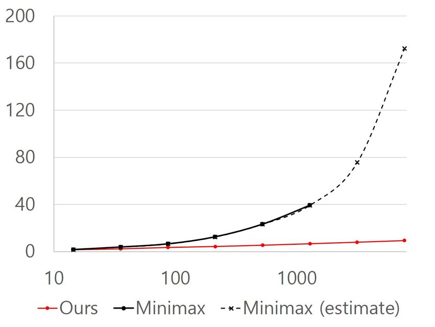
delegation of machine learning (ML) algorithms based on HE, in particular,
has garnered much attention since many ML algorithms are being utilized for
personal data, and privacy-related issues are constantly being raised.
    However, HE serves only limited types of operations: addition and multipli-
cation. It has been a challenging problem to compute a general circuit containing
sophisticated non-polynomial functions based on HE. The most prevalent solu-
tion for this is to replace non-polynomial functions with its polynomial approx-
imations. An evaluator of HE first selects the domain of each real-valued non-
polynomial function and replaces the function with its polynomial approximation
on the selected domain interval. This enables us to approximately compute any
given circuit in encrypted states, and now we focus on a specific problem that is
to find an appropriate polynomial approximation for HE.
    Meanwhile, a computation over encrypted data has several differences com-
pared to that in an unencrypted state. First, the evaluator of HE cannot observe
the input values; moreover, the intermediate values during the evaluation should
not be revealed. As a consequence, there are only a few clues about the domain
interval of each real-valued function. Also, all intermediate values during the
evaluation should belong to the plaintext space of HE. Once a single intermedi-
ate value gets out of the plaintext space of HE, it has the potential to ruin the
ciphertext and damage all evaluation results. Therefore, we should find polyno-
mial approximations on large domain intervals for successful evaluations based
on HE.

1.1    Fundamental Problem

The approximation error induced by the polynomial approximation determines
the quality of computation. To use a polynomial approximation for the privacy-
preserving computation based on HE, we should consider both (a) the error
induced by the polynomial approximation and (b) the computational cost for the
evaluation of the polynomial approximation function. For ease of discussion, in
this paper, we aim to minimize the computational cost of approximate evaluation
of a real-valued function in an encrypted state under a given fixed maximum
error. Ultimately, the approximate evaluation with a small error and a small
computational cost is the most desirable.
    For the computational cost, we take the number of multiplications into ac-
count as a top priority. This is because, in HE computation, the multiplication
between two ciphertexts is much heavier than the other homomorphic opera-
tions such as addition, subtraction, and constant multiplication. We stress that
the evaluation of a polynomial with a higher degree does not necessarily require
more number of multiplications.3 Our goal here is to minimize the computational
costs during the approximate computation; rather than to minimize the degree
of an approximate polynomial.
3
    For instance, we can compute a polynomial x8 = ((x2 )2 )2 with 3 multiplications
    while we should use at least 4 multiplications to compute x7 .
To put it all together, the substantial question is how to evaluate a non-
polynomial real-valued function over homomorphically encrypted data with the
smallest number of multiplications. However, as we point out, HE evaluation
requires a sufficiently large domain interval to guarantee the success of the eval-
uation. While there have been some general solutions for this question, they
induce too much computational overhead as we select the sufficiently large do-
main intervals. In this paper, we focus on the following question:
On a large domain interval, how to approximately evaluate a non-polynomial
real-valued function over homomorphically encrypted data with a less number of
homomorphic multiplications?
In this paper, we provide a partial solution to the question. For example,
our solution enables us to evaluate the logistic function at large intervals with
reasonable costs in encrypted states. With the previous approach, such as the
combination of√minimax approximation and Paterson-Stockmeyer algorithm, we
should use Ω( R) multiplications for the approximate evaluation with fixed
maximum error on the domain interval [−R, R]. Our solution, domain-extension
methodology, enables us to use O(log R) multiplications to approximately evalu-
ate the logistic function on domain interval [−R, R] with a fixed maximum error
in encrypted states.
More generally, our domain-extension methodology serves an efficient privacy-
preserving evaluation of functions that converge at infinities (i.e. the limit of
σ(x) exists as x → ±∞). By using our methodology, we can approximately √
evaluate with a fixed maximum error those functions on [−R, R] with O( R)
multiplications in encrypted states. To the best of our knowledge, this is compu-
tationally better than the combination√of minimax approximation and Paterson-
Stockmeyer algorithm, which uses Ω( R) multiplications.
In addition, our methodology can be utilized for the management of outliers
from the outside of the approximation interval during the privacy-preserving
computation. Even a few outlying data can destroy the result because the eval-
uation value of polynomials can easily escape the plaintext space of HE at the
outside of a fixed domain interval. However, selecting a huge approximation in-
terval to contain all possible outliers induces too many computational overheads
and makes the computation impractical. By exploiting our methodology, we can
accommodate the rare outliers from a sufficiently large interval [−R, R] by using
O(log R) additional multiplications.
1.2 Our Contributions
Our contributions can be formalized as follows.
• Domain-extension methodology We propose a domain-extension method-
ology, which efficiently extends the valid domain interval of a polynomial for
HE. We first suggest the concept of domain extension functions (DEFs) and
domain extension polynomials (DEPs), which extend the valid domain in-
terval by a factor of L, the extension ratio (i.e., extend the domain intervalfrom [−R, R] to [−LR, LR]). In contrast to a simple scaling, DEFs and DEPs preserve the feature of the original function on its original domain interval. Domain-extension methodology consists in using DEFs and DEPs repeat- edly. After n domain-extension processes, we can extend the domain interval by a factor of Ln while preserving the feature of the original function on its original domain interval. As a consequence, once we are given a function on a small interval [−r, r], we can utilize it on a wider domain interval [−R, R] by using O(log R) additional operations; We note that the extended function behaves similarly on the original domain interval [−r, r]. • Uniform approximation on wide intervals. By using domain-extension methodology, we suggest an efficient way to evaluate in encrypted state a function f (·) that converges at infinities, i.e., limx→∞ f (x) and limx→−∞ f (x) exist in R. Our method provides a uniform polynomial approximation of f (·) on [−R, R] that can be evaluated by O(log R) multiplications and O(1) mem- ory in encrypted state. In terms of computational complexity, this is much better than the previous approach, minimax approximation and Paterson-Stockmeyer algorithm. We observe that the degree of the minimax approximation on [−R, R] is Ω(R) in cases of functions that converges at infinities. √ As a result, during√the computation in encrypted states, it requires Ω( R) operations and Ω( R) memory space, and it is inefficient to use it for sufficiently large R. In con- trast, our method can be evaluated with O(log R) operations and is more practical. We also implement and compare both methods in Section 5.1. • Accommodation of outliers from wide intervals. While using HE for numerous data, a single unexpected datum has the potential to damage the entire result. This is because an evaluation of a polynomial at the out of a fixed interval can easily get out of the plaintext space of HE. This immediately contaminates the ciphertext and ruins all evaluation results. However, it seems to be inefficient to use polynomial approximations on huge approximation intervals that are capable to contain all outliers. On the other hand, by using the domain-extension method, we can efficiently accommodate the rare outliers from large intervals. Our method accommo- dates the outliers from a large interval [−R, R] by using O(log R) additional operations, and prevents the rare outliers from ruining the entire process. • Logistic regression over large datasets in encrypted state. We ap- ply our method to perform the privacy-preserving logistic regression for big datasets based on HE. By applying our method to the logistic function, we efficiently evaluate the logistic function on large domain intervals in an encrypted state. There have been several similar works to this, but to the best of our knowledge, they are unlikely to be applied to big datasets. All previous works heuristically selected the domain interval of the logistic func- tion, and we observed that those short intervals are not sufficient for many big public datasets. Moreover, previous works select the domain intervals by monitoring the process in an unencrypted state; however, this monitoring
is undesirable in HE applications since it may leak some pieces of informa-
      tion about the data. In this work, on the other hand, we approximate the
      logistic function on sufficiently large domain intervals by using DEPs. This
      enables us to successfully perform the logistic regression on heavy datasets
      with various hyper-parameters in encrypted states.

1.3     Related Work

1.3.1 Machine Learning over Encrypted Data For the privacy-preserving
delegation of computation, many works have applied HE to ML algorithms. The
key to HE-based solutions for privacy-preserving ML algorithms is appropri-
ate replacement of real-valued functions by their polynomial approximations.
Since logistic regression has a simple structure, there have been several works
that leverage HE for the privacy-preserving logistic regression [1–4]. Kim et al.
proposed a HE-based logistic regression [2]. They replace the logistic function
with the least square fitting polynomial approximation on [−8, 8]. Chen et al.
implement HE-based logistic regression by using the minimax polynomial ap-
proximation on [−5, 5] [3]. To make input values of the logistic function belong
to [−5, 5], they perform preprocessing (average pooling) to the data. Han et al.
use the least square fitting polynomial approximation on [−8, 8], and also per-
form preprocessing (average pooling) for the experiment on MNIST dataset [4].
To the best of our knowledge, all previous works heuristically select the approx-
imation interval of the logistic function. In some cases, preprocessing is needed
to force the inputs of the logistic function to belong to the selected interval.
This selection of short approximation intervals makes it difficult to perform the
logistic regression on large public datasets such as the Swarm Behavior dataset.
In this work, we suggest a practical solution to approximate the logistic func-
tion on substantially wide intervals, and by using it, we implement the logistic
regression in an encrypted state for large datasets.
    There also have been many works that utilized HE to ML algorithms other
than the logistic regression. CryptoNet modified CNN models to be HE friendly
by replacing the ReLU function and max-pooling by square function and sum
function respectively [5]. Hesamifard et al. suggested a better polynomial re-
placement of the ReLU function and analyzed its efficiency [6].

1.3.2 Computation with less multiplications When we use HE, multipli-
cation is much heavier than the other operations such as addition and constant
multiplication. Thus, the evaluation of a polynomial by using a less number of
multiplications is important to mitigate the computational overhead from HE.
    Paterson-Stockmeyer √algorithm is an algorithm to evaluate a polynomial
of degree d by using O( d)multiplications [7]. Chen et al. adopted Paterson-
Stockmeyer algorithm for the HE computations, and they performed Paterson-
Stockmeyer algorithm based on the Chebyshev basis to make the coefficients
more consistent [8]. Chen et al.’s algorithm is being widely used for the evalua-
tion of high-degree polynomials based on HE [9, 10].
On the other hand, while Paterson-Stockmeyer algorithm provides good per-
formances on general polynomials, there exist some polynomials that can be
evaluated with less number of multiplications compared to Paterson-Stockmeyer
n
algorithm. For example, x2 can be evaluated with only n multiplications by
repeating the squaring, rather than 2n/2+1 multiplications. Finding an approxi-
mate polynomial that can be evaluated with less multiplications can reduce the
computational cost. As another example, Cheon et al. [11] proposed an itera-
tive method to approximately evaluate the sign function on [−1, 1], and they
argued that their method requires relatively less number of multiplications. In
the same manner, we suggest an iterative method for the polynomial approxi-
mation on a large domain interval, which can be evaluated with a less number
of multiplications.
1.3.3 Homomorphic Evaluation with Bit-wise HE We are focusing on
the homomorphic evaluation of functions on large domain intervals by using
HE. We point out that bit-wise HE schemes, which encrypt each bit of message
separately, induce a serious computational and memory overhead when applied
to arithmetic operations on real-valued data on large scales. Another variant
of HE schemes is programmable TFHE schemes [12, 13]. It can deal with a
slightly larger interval compared to the original TFHE scheme but still suffer
from the inefficiency of real-valued addition and multiplication [14]. There have
been several works on conversion between TFHE and CKKS scheme to address
this issue [15, 14]. However, they still have weaknesses to be applied to real-valued
functions on large domain intervals. We describe more details in Section 4.1.2.
2 Preliminaries
2.1 Notations
In this paper, Clim is the class of continuous functions that converges at infinities
(i.e., Clim := {f (·)| f (·) is continuous, and both limx→∞ f (x) and limx→−∞ f (x)
exist in R}. When we say multiplication, it means a non-scalar multiplication
unless we indicate. A maximum error between two function f (·) and g(·) on an
interval I is ∥f − g∥∞,I := sup{|f (x) − g(x)| : x ∈ I}. We omit I unless it is
necessary.
For the homomorphic encryption, we use the ring R = Z[X]/(X N + 1) where
N is a power-of-two integer, and Rq denotes R/qR.
2.2 Homomorphic Encryption and CKKS scheme
HE is a cryptographic scheme that allows operations in encrypted states with-
out any decryption process. Among various HE schemes, we adopted CKKS
scheme presented by Cheon at el [16, 17], which supports arithmetic operations
of approximate numbers. CKKS scheme has a strong advantage in application to
machine learning algorithms since its plaintexts are real numbers. CKKS schemehas been adopted in many implementations of privacy-preserving machine learn-
ing algorithms based on HE [4, 18, 19].
Let N be a power-of-two integer. There exists a field isomorphism τ : R[X]/(X N +
1) → CN/2 which CKKS scheme uses for encoding and decoding messages.
CKKS scheme encrypts a (encoded) plaintext m ∈ CN/2 into a ciphertext
ct ∈ RQ . For the decryption process, a secret key sk is needed; formally, the
decryption process is
Decsk (ct) = m + e,
where e is a small error vector. We refer [16] for the detail of CKKS scheme. The
main operations of CKKS scheme and their properties are the followings.
• Add(ct1 , ct2 ): For ciphertexts ct1 and ct2 of m1 and m2 , output a ciphertext
ct of m1 + m2 .
• cMult(m, ct1 ): For a ciphertext ct1 of m1 and a message m, output a cipher-
text ct of m ⊙ m1 .
• Mult(ct1 , ct2 , evk): For ciphertexts ct1 and ct2 of m1 and m2 , output a cipher-
text ct of m1 ⊙ m2 , where ⊙ indicates the component-wise multiplication
between messages in CN/2 .
• Bootstrap(ct, evk): For ciphertexts ct of m, output a ciphertext ct′ of m with
a fresh noise level.
Each multiplication between ciphertexts increases the noise in ciphertexts, so
it is necessary to refresh the noise level by using Bootstrap after consuming some
multiplicative levels. Also, Bootstrap and the Mult are significantly slower than
other operations. Thereby, the number of multiplications and the multiplica-
tive depth mostly determines the computational costs of circuits over CKKS
ciphertexts.
To use CKKS scheme, we should select the parameters N and qL , where N
is the dimension of the ring RqL and qL is the initial modulus size.
2.3 Minimax Polynomial Approximation and Paterson-Stockmeyer
Algorithm
For a given continuous function f (·), an interval [a, b] and a positive integer d,
a minimax polynomial approximation p(·) is a polynomial of degree at most d
such that minimize the maximum error, ∥f − p∥∞,[a,b] . Many algorithms finding
the minimax polynomial approximation have been suggested such as Remez
algorithm and Barycentric-Remez algorithm [20, 21].
Minimax approximation guarantees a good quality of approximation at each
point of the approximation interval. Hence, it is plausible to be adopted in the
polynomial approximation for HE computations which hide the inputs of each
function to the HE evaluator.
The evaluation of a high-degree polynomial requires lots of multiplications
and additions. There are several evaluation algorithms such as Horner’s method [22]
and Paterson-Stockmeyer algorithm [23] to decrease the computational costs ofthe evaluation. Horner’s method √ requires O(d) multiplications, and Paterson-
Stockmeyer algorithm requires O( d) multiplications. Paterson-Stockmeyer al-
gorithm is often being adopted when multiplication is substantially more ex-
pensive than addition operation; such as circuits over matrix and circuits over
HE.
Chen et al. [8] suggest Paterson-Stockmeyer algorithm with Chebyshev ba-
sis. They pointed out that in the case of many known polynomial approximation
techniques, the coefficient with respect to the Chebyshev basis is more consis-
tent compared to that with respect to the power basis. The modified Paterson-
Stockmeyer algorithm is currently widely being used for the evaluation of high
degree polynomials based on HE.
2.4 Logistic Regression
The logistic regression algorithm is a well-known ML algorithm that solves binary
classification problems. A logistic regression classifier consists of a weight w and
a bias b. As in [2, 24], for the ease of discussion, we use each datum with an
additional feature with the value of 1 for the bias term. To be more detailed,
we represent each datum x in the form of z = (x, 1), and the logistic regression
model in the form of W = (wT , b)T . Then, wT x + b = W T z.
For the inference of the logistic regression, a model W classifies each datum
x into a class of either one of 1 or −1 by addressing the value of the following.
Pr the label of x is 1 = σ(W T z)
where σ(t) = 1/(1 + e−t ) is the logistic function.
For the training of logistic regression, we consider a cost function
1 X
J(W ) = log(1 + exp(−y · W T z))
n
(z,y)
where each z is a datum with the class of y ∈ {−1, 1}, and n is the number
of data. By using gradient descent method to this cost function, the training
process seeks the appropriate weights and bias that minimize the cost function
for given training dataset. Explicitly, for a given learning rate α, we update the
weight and bias as follows.
α X
W ← W − α∇J(W ) = W + σ(−y · W T z) · (yz)
n
(z,y)
3 Domain-extension Methodology
HE supports only polynomial operations: addition and multiplication. When we
compute a circuit over encrypted data based on HE, we need to replace the
non-polynomials by their polynomial approximations on each of its estimateddomain interval, the approximation interval. Once the intermediate value during
the computation gets out of the plaintext space of HE, the outlier immediately
ruins the ciphertext and contaminates the entire computation. To avoid this, we
need to select the approximation interval of each polynomial approximation as
large enough. Unfortunately, a larger approximation interval requires a bigger
degree of the approximate polynomial, and results in considerable computational
overhead.
We can efficiently evaluate low-degree polynomials, but in general, a low-
degree polynomial is useful only on relatively small domain intervals and be-
haves unexpectedly on the out of the small interval. In this work, we aim to
utilize a low-degree polynomial to large intervals by using a few more number of
operations. We call this process by domain-extension process. By the domain-
extension process, we use a low-degree polynomial similarly on its original (small)
domain interval; meanwhile, on a larger interval, we maintain the size of function
values bounded and prevent it from behaving unexpectedly.
For ease of discussion, during the domain-extension process, we distinguish
two domain intervals of a given polynomial, the interval type I and II. We denote
the interval type I as the interval that the function after the domain-extension
process behaves similar to the original polynomial. We denote the interval type
II as the interval that the size of function values is reasonably bounded. More
precisely, We aim to extend the interval type II during the domain-extension
process. The maximum norm (i.e., l∞ -norm) of the function after the domain-
extension process on the extended interval type II is bounded by that of the
original function on the original interval type II. In short, we regard interval
type I as where the most of inputs come from, and interval type II, on the other
hand, is the interval where we want to prevent the function value from behaving
unexpectedly.
3.1 Motivation
Domain Extension Function. We first introduce domain extension functions
(DEFs). For a given L > 1, we define a function D : [−L, L] → [−1, 1] by
Fig. 1: An example of domain-extension process by using a DEF.1
D(x) = 2 |x + 1| − |x − 1| . We will call this function a DEF with an extension
ratio L.
Now assume that we are given a function P (·) with the domain [−1, 1]. Then,
on [−L, L], the composition P ◦ D(·) behaves as followings.
P (−1),
if − L ≤ x ≤ −1
P ◦ D(x) = P (x), if − 1 ≤ x ≤ 1
P (1), if 1 ≤ x ≤ L
This means that interval type II of P ◦ D is extended to [−L, L] while the
function values do not change on the interval type I, [−1, 1].
Figure 1 illustrates the feature of DEF with extension factor 5, and how it
extends the small interval type II [−1, 1] of a polynomial 4x3 − 3x to a wide
interval [−5, 5]. In particular, it extends the interval type II by simply stretching
the endpoints, and it exactly preserves the features on the interval type I.
Domain-extension Methodology. We can extend the size of the interval type
II exponentially by repeatedly using the argument above. To be more precise,
let D(·) be a DEF with the extension factor L that extends interval type II
[−1, 1] to [−L, L]. We may consider the scaled function Dn (x) := Ln D(x/Ln )
as another DEF with extension ratio L, which extends the interval type II from
[−Ln , Ln ] to [−Ln+1 , Ln+1 ]. Applying Di (·) n times sequentially, we can extend
interval type II of f (·) from [−1, 1] to [−Ln , Ln ]. In other words, we extend the
size of interval type II by factor of R with O(log R) domain-extension processes.
We also point out that the function value on the original domain, [−1, 1], does
not change.
We name this iterative strategy that extends the interval type II while pre-
serving the features of the target function on the interval type I as domain-
extension methodology. Unfortunately, DEFs may not be directly used for privacy-
preserving computations based on HE since they cannot be evaluated by using
only HE operations. Thus, we define domain extension polynomials (DEPs) in
Section 3.2, and we explain the domain-extension methodology with DEPs in
Section 3.3.
Fig. 2: An example of DEP.Fig. 3: An example of domain-extension process by using a DEP.
3.2 Domain Extension Polynomial
To utilize domain-extension methodology for the HE-based computations, we
need polynomials that can take the role of DEFs. The crux is to exploit the
approximate polynomials of DEFs. For ease of discussion, we define a narrow
definition of DEPs as follows.
Definition 1 (Domain Extension Polynomials). For given constants R2 >
R1 > r > 0 and small error δ > 0 , we define D(δ, r, R1 , R2 ) as a class of
polynomials d(·) satisfying:
(a) |x − d(x)| ≤ δ|x|3 ∀x ∈ [−r, r]
(b) 0 ≤ d′ (x) ≤ 1 ∀x ∈ [−r, r]
(c) d(r) < d(x) < R1 ∀x ∈ [r, R2 ]
(d) −R1 < d(x) < d(−r) ∀x ∈ [−R2 , −r].
We call R2 /R1 as the extension ratio of d(·). We also denote d(·) is a DEP
extending [−R1 , R1 ] to [−R2 , R2 ] preserving [−r, r] if d(·) ∈ D(δ, r, R1 , R2 ).
Figure 2 visualizes a graph of an example of DEPs. We point out that it
approximates a DEF and it may behave similarly to a DEF. Figure 3 visualizes
how a DEP (approximately) extends the interval type II of a given polynomial.
We can observe that a DEP can extend the interval type II of a polynomial
while preserving the function values on the narrow interval type I with minor
differences. More precisely, we argue that a DEP d(·) ∈ D(δ, r, R1 , R2 ) can extend
the interval type II of a polynomial from [−R1 , R1 ] to [−R2 , R2 ] while preserving
the polynomial on a narrow subinterval of type I, [−r, r]. We formally state this
in Theorem 1.
Theorem 1. Assume that we are given a DEP d(·) ∈ D(δ, r, R1 , R2 ), and a
polynomial p(·) such that sup{|p′ (x)| : −r ≤ x ≤ r} ≤ M . Then,
∥p ◦ d ∞,[−R2 ,R2 ]
≤ ∥p∥∞,[−R1 ,R1 ] ,
∥p ◦ d − p ∞,[−r,r]
≤ M r3 δ,
and
sup{|(p ◦ d)′ (x)| : −r ≤ x ≤ r} ≤ M.Proof. For each x ∈ [−r, r], there exist x∗ between d(x) and x such that
|p ◦ d(x) − p(x)| = |p′ (x∗ )||x − d(x)| ≤ M δ|x|3 ≤ M r3 δ.
Also,
|(p ◦ d)′ (x)| = |p′ (d(x))d′ (x)| ≤ M.
Note that 0 ≤ d′ ≤ 1 on [−r, r] insists that −r ≤ −|x| ≤ d(x) ≤ |x| ≤ r.
To put it all together, a DEP behaves similar to a DEF. A DEP extends the
interval type II from [−R1 , R1 ] to [−R2 , R2 ], while preserving the features of the
original function on a small subinterval of type I, [−r, r].
3.3 Domain-extension Methodology with DEPs
We now describe an iterative domain-extension by using a DEP.
We begin with the observation that if d(·) is a DEP that extends [−R1 , R1 ] to
[−R2 , R2 ], then its scaled polynomial kd(·/k) is a DEP that extends [−kR1 , kR1 ]
to [−kR2 , kR2 ].
Theorem 2. If d(·) ∈ D(δ, r, R1 , R2 ) and L > 1, then
x δ
D(x) := Ld ∈ D 2 , r, LR1 , LR2 .
L L
Proof. For each x ∈ [−r, r], let z = x/L ∈ [−r, r]. Then,
δ
|x − D(x)| = |Lz − Ld(z)| ≤ Lδ|z|3 = |x|3
L2
holds. Also,
d x
D′ (x) = Ld = d′ (x) ∈ [0, 1].
dx L
For each x ∈ [r, LR2 ], let z = x/L ∈ [−r/L, R2 ]. If z ≤ r, d Lr ≤ d(z)
≤ d(r) ≤
R1 holds since 0 ≤ d′ ≤ 1 on x ∈ [0, r]. Meanwhile, if z > r, d Lr ≤ d(r) ≤
d(z) ≤ R1 holds. Thus, in both cases,
r
D(r) = Ld ≤ Ld(z) = D(x) ≤ LR1
L
holds for x ∈[−LR2 , −r].
holds, and similar result
Therefore, D(x) ∈ D Lδ2 , r, LR1 , LR2 .
By using Theorem 2, we can generate a sequence of DEPs, Bn (x) = Ln B(x/Ln ),
from a base DEP B(x) that extends [−R, R] to [−LR, LR]. Each DEP Bn (·) ex-
tends [−Ln R, Ln R] to [−Ln+1 R, Ln+1 R], so we can utilize them sequentially. To
apply DEPs Bi (·) sequentially to a given polynomial that has interval type IIFig. 4: The functions with extended intervals type II after 1, 2, 3 iterations of
domain-extension method to the red curve. Note that the feature of the original
function is preserved on [−0.5, 0.5]
[−R, R], the interval type II would be extended to [−Ln R, Ln R] after n itera-
tions. Hence, we can extend the interval type II by a factor of L′ with O(log L′ )
iterations. Figure 4 visualizes how the sequence of DEPs extends the interval
type II for each iteration. We will call this methodology as domain-extension
methodology. We argue that domain-extension methodology with DEPs (1) ex-
tends the interval type II efficiently, and (2) preserves the feature of the original
function on the interval type I.
Theorem 3 (Domain-extension methodology). Assume that B(·) ∈ D(δ, r, R, LR)
and a polynomial p(·) on [−R, R] is given. For each non-negative integer n, let
x
Bn (x) := Ln B .
Ln
Then, after n sequential composition of Bi (·) to p(·),
p ◦ B0 ◦ · · · ◦ Bn−1 ≤ ∥p∥∞,[−R,R] ,
∞,[−Ln R,Ln R]
and
L2
p − p ◦ B0 ◦ · · · ◦ Bn−1 ≤ M r3 δ
∞,[−r,r] L2−1
holds where M = sup{|p′ (x)| : −r ≤ x ≤ r}.
Proof. By Theorem 2, Bn (·) ∈ D              δ        n
                                            L2n , r, L R, L
                                                            n+1
                                                                R       . By using Theorem 1,
we conclude that

              p − p ◦ B0 ◦ · · · ◦ Bn−1
                                  n−1
                                  X
             ≤ ∥p − p ◦ B0 ∥ +          ∥p ◦ B0 · · · ◦ Bi−1 − p ◦ B0 · · · ◦ Bi ∥
                                  i=1
                        n−1                  ∞
                        X      1            X    1         L2
             ≤ M r3 δ          2i
                                  ≤ M r 3
                                          δ      2i
                                                    = M r3 2   δ
                        i=0
                              L             i=0
                                                L         L −1

Here, we denoted ∥ · ∥∞,[−r,r] as ∥ · ∥.

    Theorem 3 implies that if we use a DEP with a small δ, the output polynomial
of domain-extension methodology has only a small difference from the original
polynomial on [−r, r], and at the same time, the output polynomial is bounded
on the large interval, [−Ln R, Ln R].
    To briefly sum up, we suggest DEPs and domain-extension methodology with
it that extends the interval type II of a polynomial efficiently while preserving
the approximation property on the interval type I. Note that to extend a poly-
nomial’s interval type II by a factor of L, domain-extension methodology uses
O(log L) operations.

Remark 1. Note that the domain-extension methodology is done by invoking a
simple base DEP repeatedly. Once we are given an appropriate base DEP B(·)
that can be stably evaluated based on HE (e.g., it does not considerably magnify
the errors induced by HE), its scaled function Bn (x) would be also HE friendly.
This makes the domain-extension methodology stable and HE friendly.

Example 1. d(x) = − 27   x + x is a DEP in D 27
                       4 3                        4
                                                    , r, 1, L for each 1.5 < L <
   √
1.5 3 and 0 < r < 1.5 such that d(r) < d(L). Note that Theorem 2 implies that
we can decrease δ as much as possible by scaling.

4   Homomorphic Evaluation on Large Intervals

In this section, we explain how domain-extension methodology can be used for
privacy-preserving computations based on HE. We remark that to exploit HE,
non-polynomial functions should be replaced by their polynomial approxima-
tions, and the approximation interval should be large enough to contain all
input values. Since polynomial approximation on the large interval, in general,
introduces a high degree and considerable computational overheads, domain-
extension methodology may provide a more efficient solution to manage a large
domain interval.
    We suggest two applications of thedomain-extension methodology. First, we
show that for several functions (e.g., the logistic, arctan, tanh, capped ReLU, and
Gaussian function), domain-extension methodology extends not only interval
type II, but also interval type I. As a consequence, by using the domain-extension
methodology, we can evaluate those functions based on HE over large domain
intervals. We stress that this is substantially more efficient than other known
polynomial approximation techniques.
Second, we explain that domain-extension methodology can effectively man-
age rare outlying data. Suppose there are some rare outliers from a large interval,
while the most of data are from a small domain interval. The function value of
known polynomial approximations soars rapidly on the outside of a fixed approx-
imation interval. An outlier from the out of the approximation interval would
become extremely large after the homomorphic evaluation of the function. Once
the evaluation value does not belong to the plaintext space of HE, the ciphertext
will be polluted, and the entire results will be contaminated. Hence, the approx-
imation interval should be large, but it might be inefficient if there are only a
few outliers. In Section 4.2, we suggest an efficient solution to address this issue
by using the domain-extension methodology.
4.1 Uniform Approximation using DEPs
We introduce an efficient polynomial approximation technique for functions in
Clim (i.e., f (·) that is continuous and both limx→∞ f (x) and limx→−∞ f (x)
exist in R). We first remark that many ML algorithms utilize functions that
converge at infinities; e.g., the logistic function, tanh function, arctan, capped
ReLU function [25], and Gaussian function. To perform those ML algorithms in
an encrypted state, it is necessary to uniformly approximate by polynomials the
functions in Clim . However, with known approaches, the HE evaluation of such
functions on sufficiently large intervals results in considerable overhead.
By utilizing our domain-extension method in Section 3, we suggest an efficient
polynomial approximation technique for functions in Clim . The idea is simple:
find an approximation on a smaller interval and extend its approximation interval
by using the domain-extension method. Then, we approximately compute f (·) ∈
Clim on [−R, R] with O(log R) operations. Algorithm 1 describes how to utilize
domain-extension methodology for this scenario.
As in Figure 4, our domain-extension methodology stretches the graph of the
given polynomial by pulling on both ends while fixing the central part (interval
type I) of the original function. Thus, in the case of approximate polynomials
of f (·) ∈ Clim , the domain-extension method immediately extends not only the
interval type II but also the interval type I, so we yield an efficient polynomial
approximation f (·) on the extended wide interval. More precisely, Theorem 4
states that Algorithm 1 is correct unless r is too small.
Theorem 4. Assume that a M -Lipshitz continuous function f (·) ∈ Clim and a
DEP d(·) ∈ D(δ, r, R, LR) such that
|f (x) − f (y)| < ϵ1 if x, y ≤ −d(r)
|f (x) − f (y)| < ϵ1 if x, y ≥ d(r).Algorithm 1 Homomorphic evaluation of Clim functions on large intervals
Input: f (·) ∈ Clim , x ∈ [−Ln R, Ln R].
Output: Approximate value of f (x).
1: P (·) := the minimax polynomial on [−R, R]
2: Take B(·) ← D(δ, r, R, LR)
3: y = x
4: for i ← n − 1 to 0 do
5: y = Li B Lyi
6: end for
7: y = P (y)
8: return y
for some ϵ1 > 0. Suppose that p(·) on [−R, R] is a polynomial approximation of
f (·) that satisfies
|f (x) − p(x)| < ϵ2 if x ∈ [−R, R].
for some ϵ2 > 0.
Then, p ◦ d(·) is a polynomial approximation of f (·) on [−LR, LR] with max-
imum error is bounded by max(M r3 δ, ϵ1 ) + ϵ2 .
Moreover, after Algorithm 1, we get the polynomial approximation on [−Ln R, Ln R]
with maximum error less than
3 2
max( MLr2 −1
L
δ, ϵ1 ) + ϵ2 .
Proof. From Theorem 1, for each x ∈ [−r, r],
|p ◦ d(x) − f (x)| ≤ |p ◦ d(x) − f ◦ d(x)| + |f ◦ d(x) − f (x)|
≤ ϵ2 + M |x − d(x)| ≤ ϵ2 + M r3 δ.
Meanwhile, for each x ∈ [r, LR],
|p ◦ d(x) − f (x)| ≤ |p ◦ d(x) − f ◦ d(x)| + |f ◦ d(x) − f (x)|
≤ ϵ1 + ϵ2 ≤ max(M r3 δ, ϵ1 ) + ϵ2 .
And the same argument holds for x ∈ [−LR. − r]. Thus,
|p ◦ d(x) − f (x)| ≤ max(M r3 δ, ϵ1 ) + ϵ2
for all x ∈ [−LR, LR].
Finally, the similar argument with Theorem 3 proves that Algorithm 1 serves
the uniform approximation on [−Ln R, Ln R] with maximum error less than
3 2
max( MLr2 −1
L
δ, ϵ1 ) + ϵ2 .
As a consequence, we can approximately evaluate a function f (·) ∈ Clim on an
3 2
arbitrarily large interval [−R, R] within the error less than ϵ = max( MLr2 −1
L
δ, ϵ1 )+Fig. 5: The graphs of a polynomial before and after the domain-extension
methodology. The black line shows the exact logistic function, the green line
shows its 9th order minimax approximation on [−14.5, 14.5], the red line shows
the polynomial after 1 domain-extension process, and the pink line shows the
polynomial after 2 domain-extension processes.
# of extensions 0 1 2 3
Size of domain 29 71.05 174.07 426.48
Maximum error 0.04416 0.04447 0.04447 0.04447
# of Mult 4 6 8 10
Table 1: The maximum errors of polynomial approximations of the logistic func-
tion using Algorithm 1 with various numbers of domain-extension processes. We
used the DEP x − 16/22707x3 , which extends [−14.5, 14.5] to [−35.525, 35.525].
ϵ2 by using Algorithm 1 with O(log R) iterations of domain-extension processes.
Table 1 and Figure 5 describe the maximum error after the domain-extension
processes for the homomorphic evaluation of the logistic function.
Our algorithm is very efficient for large domain intervals. We measured the
computational cost in terms of the number of multiplications during the com-
putation, because the multiplication is much heavier than other operations in
HE. To approximately evaluate a function in f (·) ∈ Clim on sufficiently large in-
terval [−R, R], we perform domain-extension process for O(log R) times; hence,
our method uses O(log R) multiplications in encrypted state. Also, we point out
that our method exploits O(1) memory since the domain-extension processes are
sequentially executed.
For the computation based on HE, the multiplicative depth is also an impor-
tant factor since it determines the number of required bootstrapping during the
computation. The multiplicative depth of our method is O(log R) since we uses
O(log R) domain-extension processes for the interval [−R, R].Remark 2. Our algorithm can be easily extended to a function whose difference
from a low degree polynomial converges to constants ∈ R at infinities. Note that
such function can be represented as f (x) + p(x), where f (·) ∈ Clim and p(·) is a
lower degree polynomial.
4.1.1 Towards higher accuracy Theorem 4 states that the domain-extension
methodology extends the approximation interval for function f (·) in Clim , while
compromising the small maximum error bounded by a certain limit. The error
growth from domain-extension process using d(·) ∈ D(δ, r, R, LR) is determined
by f , δ and r. To yield higher accuracy, e.g., maximum error less than 2−20 , with
Algorithm 1, domain-extension polynomials with small δ’s are needed. We intro-
duce optimizations that enable us to use simple domain-extension polynomials
with not too small δ’s for high precision polynomial approximations.
Suppose we want to approximate a function f (·) ∈ Clim on a large domain
interval [−R, R]; by using DEP d(·) and a polynomial approximation on the
small interval [−r, r].
Our first optimization is to use the minimax approximation Q(·) of f ◦ d−1 (·)
on [−r, r] instead of the minimax approximation P (·) of f (·) on [−r, r]. To be
more precise, let Q(x) ≈ f ◦d−1 (x) where d−1 ◦d(x) ≈ x, and suppose the degree
of Q(·) and P (·) are equal. Then,
∥f − P ◦ d∥∞,[−R,R] ≥ ∥f ◦ d−1 − P ◦ d ◦ d−1 ∥∞,[−r,r]
≈ ∥f ◦ d−1 − P ∥∞,[−r,r]
≥ ∥f ◦ d−1 − Q∥∞,[−r,r]
≈ ∥f − Q ◦ d∥∞,[R,R] .
To sum up, we can expect to yield a better maximum error than that in Theo-
rem 5 by considering the minimax approximation of f ◦ d−1 (·).
However, finding the minimax approximation of f ◦ d−1 (·) is not easy in
general. To address this issue, we suggest a second heuristic optimization. The
idea is to use the polynomial approximation of d−1 , say q(x). Then, f ◦ d−1 (x) ≈
P ◦ q(x). By applying domain-extension methodology to P ◦ q(·), we get P ◦ q ◦
d ≈ f ◦ d−1 ◦ d ≈ f . Thus, we can yield an efficient high precision polynomial
approximation on large domain intervals.
Fortunately, a low degree polynomial approximation of d−1 (·) is sufficient to
achieve a high accuracy (e.g., maximum error ≤ 2−20 ). Algorithm 2 describes an
algorithm of our method for high accuracy using the simplest domain-extension
4 3 th
polynomial, x − 27R 2 x . For the optimization, we use a 5 degree polynomial,
2 2n
4 L (L −1) 3 5
q(x) = x + 27 L2n (L2 −1) (x − x ), which is a polynomial approximation of a
composition of inverse of n DEPs used for the domain-extension method. We
implemented Algorithm 2 to approximate the logistic function on large domain
intervals within maximal error 2−20 . The experimental results are represented
in Figure 6 and Table 2. The detailed results are reported in Section 5.Algorithm 2 Homomorphic evaluation of Clim functions on large intervals with
higher accuracy
Input: f (·) ∈ Clim , x ∈ [−Ln R, Ln R].
Output: Approximate value of f (x).
1: P (·) := the minimax polynomial on [−R, R]
2: y = x
3: for i ← n − 1 to 0 do
4 3
4: y = y − R2 27L 2i y
5: end for
6: y = y/R
2 2n
4 L (L −1) 3 5
7: y = y + 27 L2n (L2 −1) (y − y )
8: y = P (Ry)
9: return y
Maximum Error (log2 )
# of extensions 0 1 2 3 4
(Size of domain) (110) (220) (440) (880) (1760)
Algorithm 1 -21.6 -14.0 -13.7 -13.6 -13.6
Algorithm 2 -21.6 -20.3 -20.1 -20.0 -20.0
Table 2: The logarithmic values of the maximum errors of polynomial ap-
proximations of the logistic function using Algorithm 1 and 2 with various
numbers of domain-extension processes. We used domain-extension polynomial
x − 4/81675x3 , which extends the interval type II from [−55, 55] to [−110, 110].
4.1.2 Comparison to the previous approaches For the privacy-preserving
evaluation of non-polynomial functions, to the best of our knowledge, there are
two approaches using: (a) the conversion between other HE schemes, and (b)
the minimax polynomial approximation. However, both are not satisfactory for
the evaluation on substantially large domain intervals.
Pegasus. Pegasus [14] proposed a conversion algorithm between TFHE and
CKKS scheme to evaluate non-polynomial functions over CKKS ciphertexts.
For a given CKKS ciphertext, Pegasus converts it into a number of TFHE ci-
phertexts, performs programmable bootstrappings of the TFHE scheme, and
repacks the TFHE ciphertexts into a CKKS ciphertext.
However, to utilize Pegasus for the function evaluation on large domain inter-
vals, a CKKS ciphertext should be converted into TFHE ciphertexts containing
messages from the large domain interval. This results in the large parameters of
the TFHE scheme and a substantial computational overhead incurs.
To be more precise, as mentioned in [14], when using Pegasus on [−q/2ϵ̃, q/2ϵ̃),
the approximation error is about Lq/(2ϵ̃n) where L is the smoothness of the non-
polynomial function, ϵ̃ is a small integer (e.g., 2), and q and n are parameters
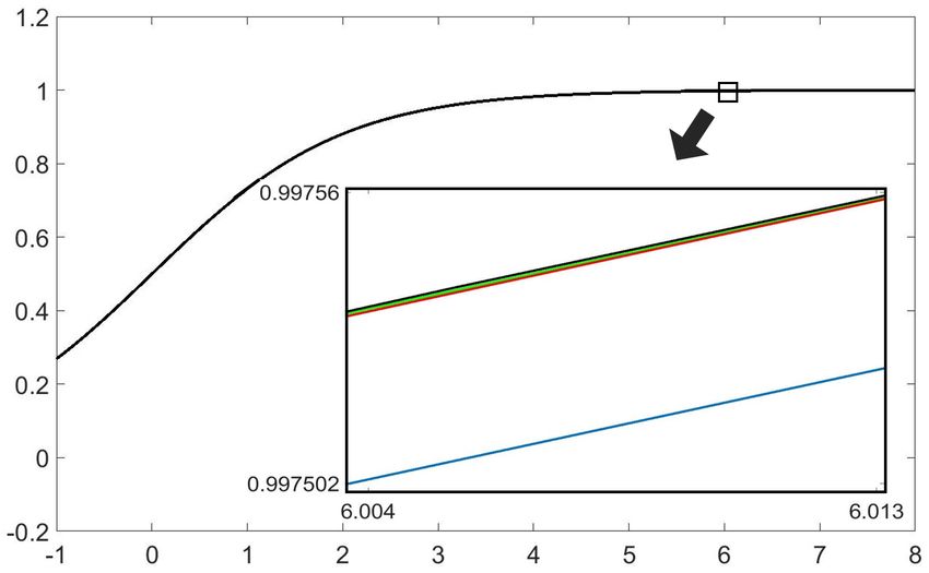
for TFHE. Thus, to evaluate on a large domain interval [−R, R] with a consis-Fig. 6: The graphs of polynomial approximations of the logistic function. The
black line shows the exact logistic function, the green line shows the 243th order
minimax approximation on [−55, 55], the blue line shows the polynomial after 3
domain-extension processes (Algorithm 1), and the red line shows the polynomial
after 3 domain-extension processes with optimization (Algorithm 2).
tent approximation error, the parameter RLWE dimension and the ciphertext
modulus should be Ω(R). This induces both the memory and computational
overhead of Ω̃(R). Pegasus mostly consider the function evaluation on narrow
domain intervals, e.g., [−8, 8].
It is also possible to use the small TFHE parameters for large domain in-
tervals. Then, instead of evaluating a function f (·) on [−R, R], one evaluates
f ( Rr x) on [−r, r]. In that case, the smoothness L of the function grows, and the
approximation error becomes large when we consider substantially large domain
intervals. We report the implementation results in Section 5.1.
Also, Pegasus generates and manipulates a TFHE ciphertext for each slot of
a given CKKS ciphertext. As a consequence, Pegasus cannot leverage the SIMD
(Single Instruction Multiple Data) operations of the CKKS scheme.
Minimax polynomial approximation. For given maximum error, minimax
approximation technique serves the polynomial approximation with the smallest
degree, so it is prevalent to use minimax approximation for HE computations. To
evaluate the minimax approximation, Paterson-Stockmeyer algorithm is being
widely adopted since it uses a less number of multiplications.
However, as we illustrate in Figure 7 and prove in Theorem 5, to approx-
imately evaluate f (·) ∈ Clim on [−R, R] in encrypted state with minimax ap-
proximation, we should compute a polynomial of degree Ω(R). As a consequence,Fig. 7: The minimal degrees for the minimax approximation to approximate the
several functions by maximum errors of 0.05 on various domains. The degree of
minimax polynomial increases linearly with respect to the size of the approxi-
mation domain.
√ √
even with Paterson-Stockmeyer algorithm, Ω( R) multiplications and Ω( R)
memory space are needed. Also, the number of cMult (multiplication between
a ciphertext and a plaintext) is Ω(R). Even though cMult is pretty faster than
Mult (multiplicatoin between two ciphertexts) in HE computation, it is not neg-
ligible when R is substantially large. We report the implementation result in
Section 5.
Theorem 5. Assume that we are given a function f (·) ∈ Clim where limx→∞ f (x) ̸=
limx→−∞ f (x). For a sufficiently small ϵ > 0, the minimax polynomial approxi-
mation on [−R, R] with maximum error ϵ has degree Ω(R) as R → ∞. Empiri-
cally, the same result holds even if limx→∞ f (x) = limx→−∞ f (x) unless f is a
constant function.
Proof. Without loss of generality, assume that limx→−∞ f (x) = 0 and limx→∞ f (x) =
1. There exists r > 0 such that |f (x) − 1| < ϵ/2 if x > r, and |f (x)| < ϵ/2 if
x < −r For sufficiently large R ≫ r, let PR (·) be the minimax polynomial ap-
proximation of f (·) on R by maximum error less than ϵ/2. Let d be the degree# of # of Mult.
Memory
Mult cMult depth
[14] √ Time: Ω(R) Ω(R)
√
Minimax Ω( R) Ω(R) Ω(log R) Ω( R)
Ours O(log R) O(log R) O(log R) O(1)
Table 3: Cost of our algorithm and previous approaches to evaluate Clim func-
tions on [−R, R] under a fixed maximum error.
of PR . Then,
ϵ ≥ sup{|PR (x) − sgn(x)| : x ∈ [−R, −r] ∪ [r, R]}
R R
= sup{|PR (rx) − sgn(x)| : x ∈ [− , −1] ∪ [1, ]}
r r r
r
r d−1
r
2 A−1 2 2 R dr
≥ (A − 1) ∼ −
πAd A+1 π dr R
where A = R/r. This
q comes from the arguments in [26].
R
This implies that dr < E for some constant E(ϵ). As a consequent, d > CR
for some constant C(ϵ), and d = Ω(R). The graphs in Figure 7 shows that the
empirical result.
Compared to the minimax approximation, our approach is more efficient in
terms of both computational and memory costs. To approximately evaluate on
[−R, R] based on HE, our method uses √ O(log R) numbers of Mult and cMult
while minimax approximation uses Ω( R) and Ω(R) number of Mult and cMult
respectively. Both methods require O(log R) multiplicative depth. See Figure 8
and 9 for the experimental results.
Also, we point out that our method uses O(1) √ memory during the computa-
tion while the minimax approximation uses Ω( R) memory for the Paterson-
Stockmeyer algorithm. Table 3 summarizes the costs to approximate a function
on [−R, R] under a fixed uniform error by using Pegasus, minimax approxima-
tion, and our algorithms.
Another point is that our method provides a stable evaluation even for large
domain intervals. This is because during the domain-extension, all we compute is
DEPs of low degrees. On the other hand, when we exploit the minimax approx-
imation with Paterson-Stockmeyer √ algorithm, we should precisely evaluate the
Chebyshev polynomial of degree d where d = Ω(R). Consequently, as R grows,
the error induced by HE would make it challenging to use Paterson-Stockmeyer
algorithm.
As more, our algorithm is much simpler to implement. In practice, it is diffi-
cult to find the minimax polynomial on a significantly large interval. In contrast,
our algorithm can be easily implemented for substantially large domain intervals,
by using a simple DEP and a minimax polynomial on a small domain interval.4.2 Accommodation of Outliers
In this section, we utilize DEPs to accommodate rare outliers distributed on a
wide interval. A polynomial approximation has a weakness to the outliers from
the outside of the approximation interval because its value soars rapidly at the
inputs from the out of the approximation interval. This can be a serious issue
since it has the potential to damage the ciphertext and ruin the entire compu-
tation. To take the training phase of neural networks in an encrypted state as
an example, a single strange training datum can generate input of an activation
function from the out of the approximation interval, and its polynomial evalu-
ation might be out of the plaintext space of HE. As a result, a single outlying
datum can destroy the ciphertext, and ruin the entire training phase. Moreover,
all the processes are being done in an encrypted state, so we even cannot detect
which datum caused the failure.
To address this issue, there should be a clever way to manage such outlying
inputs from wide intervals. However, it is inefficient to use a polynomial approxi-
mation on huge approximation intervals to manage all such outliers. We suggest,
instead, considering a polynomial approximation that is accurate on a relatively
small interval (interval type I) and bounded on a huge interval (interval type
II) at the same time. The rare outliers from the huge interval may not produce
meaningful results; albeit, they do not damage either the ciphertext or other
parts of the algorithm. For example, in the case of the neural network training
over encrypted data, we now can prevent abnormal data from contaminating the
entire process.
For the formal description, we consider F , a class of approximate functions
of f (·), as followings. We note that this is a class of approximate polynomials
that is accurate on a small interval [−r, r], and bounded by ρ on the large interval
[−R, R].
Definition 2. For a given function f (·) on [−R, R] and given R > ρ > r > 0
with small ϵ > 0 , we define F (f ; ϵ, r, ρ, R) to be a class of function of p(x)
satisfying:
(a) |p(x) − f (x)| < ϵ ∀x ∈ [−r, r]
(b) |p(x)| < ρ ∀x ∈ [−R, R].
F (f ; ϵ, r, ρ, R) is a class of functions that is accurately approximates f (·) on
[−r, r] and is bounded by ρ on [−R, R]. Thus, the HE evaluation on [−r, r] would
be valuable, and that on [−R, R] would be stable (i.e., each function value on
[−R, R] belongs to the plaintext space of HE).
In this case, our domain-extension methodology can be applied; as we regard
[−r, r] as the interval type I and [−R, R] as the interval type II. Theorem 3
explains how domain-extension methodology enables us to efficiently increase
the stable interval. Note that Theorem 6 is an immediate outcome of Theorem 3.
Theorem 6. Assume that we are given a function f (·) and its approximation
p(·) ∈ F (f ; ϵ, r, ρ, R); also, suppose we are given a DEF d(·) ∈ D(δ, r, R, LR)where LR > R > ρ > r > 0 and δ, ϵ > 0 are small. Then,
p ◦ d(·) ∈ F f ; ϵ + M r3 δ, r, ρ, LR
where M = sup{|p′ (x)| : −r < x < r}. Moreover, if we let
x
Bn (x) := Ln d n
L
for each non-negative integer n, then
L2
F ◦ B0 ◦ · · · ◦ Bn−1 (·) ∈ F f ; ϵ + M r3 δ, r, ρ, Ln
R .
L2 − 1
To put it all together, when we use a polynomial approximation in F , we can
manage the outliers from a wide interval [−R, R] by using additional O(log R)
number of operations.
5 Experiments
In this section, we implement our domain-extension methodology and apply it
to the privacy-preserving logistic regression based on HE. Note that the training
and inference of a logistic regression classifier can be done by the computation
of linear operations and the logistic function.
The logistic function is in Clim , so domain-extension methodology provides
an efficient uniform approximation of the logistic function on large intervals as
described in Section 4.1. We implement our domain-extension methodology for
the logistic function, and by using it, we perform the logistic regression based on
HE. We adopt CKKS scheme [16, 17] among many HE schemes since it supports
floating-point operation on real numbers.
We introduce two experiments: (1) homomorphic evaluation of the logis-
tic function on large domain intervals by using our methods, and (2) privacy-
preserving training of logistic regression by using our method.
We approximately evaluate the logistic function on various domain inter-
vals by using each method. Our experiments include approximation for both
moderate (i.e., maximum error≈ 0.045) and high (i.e., maximum error ≤ 2−20 )
accuracy.
For the privacy-preserving logistic regression, we used two datasets: MNIST
and Swarm Behavior datasets. For the MNIST dataset, all data belong to a
bounded interval, [0, 255]28×28 , and we approximate the logistic function on a
sufficiently large input domain that contains all the possible inputs. The Swarm
Behavior dataset, on the other hand, contains the data of values without an ex-
plicit bound. We approximate the logistic function on a sufficiently large domain
interval, [−7683, 7683]. We stress that for the Swarm Behavior dataset, as we
observed the intermediate values during the training in an unencrypted state,
the approximation interval of the logistic function should be large enough, i.e.,
larger than [−1333, 1333].You can also read