Enemies of the people - Gerhard Toews Pierre-Louis V ezina September 14, 2018
←
→
Page content transcription
If your browser does not render page correctly, please read the page content below
Enemies of the people

                                          Gerhard Toews†
                                        Pierre-Louis Vézina‡

                                        September 14, 2018

                                                Abstract

       Enemies of the people were the millions of intellectuals, artists, businessmen, politicians,
       professors, landowners, scientists, and affluent peasants that were thought a threat to
       the Soviet regime and were sent to the Gulag, i.e. the system of forced labor camps
       throughout the Soviet Union. In this paper we look at the long-run consequences of
       this dark re-location episode. We show that areas around camps with a larger share of
       enemies among prisoners are more prosperous today, as captured by night lights per
       capita, firm productivity, wages, and education. Our results point in the direction of a
       long-run persistence of skills and a resulting positive effect on local economic outcomes
       via human capital channels.

       JEL CODES: O15, O47
       Key Words: human capital, productivity, gulag, persistence, natural experiment.

   ∗
      We are grateful to Sascha Becker, Richard Blundell, Sergei Guriev, Alex Jaax, Andrei Markevich,
Tatjana Mikhailova, Karan Nagpal, Elena Nikolova, Judith Pallot, Elias Papaioannou, Helena Schweiger,
Michele Valsecchi, Thierry Verdier, and Ekaterina Zhuravskaya. We also wish to thank seminar participants
at the 2017 Journees LAGV at the Aix-Marseille School of Economics, the 2017 IEA Wold Congress in
Mexico City, the 2017 CSAE conference at Oxford, and at SSEES at UCL, NES in Moscow, Memorial in
Moscow, ISS-Erasmus University in The Hague, the OxCarre brownbag, the QPE lunch at King’s, the Oxford
hackaton, and at Saint Petersburg State University for their comments and suggestions. We are also thankful
to the Riesen and Toews families for their insightful comments received at their annual family reunion. Both
families were relocated to Kazakhstan in the 1930s and 1940s where their descendants remained until 1989.
This project has been supported by a British Academy/Leverhulme small research grant and OxCarre. We
thank Anthony Senior at King’s for help with the grant application. Finally, we also thank Eugen Ciumac
for excellent research assistance.
    †
      New Economic School, Moscow. Email: gtoews@nes.ru.
    ‡
      Dept of Political Economy, King’s College London. Email: pierre-louis.vezina@kcl.ac.uk.
The FAKE NEWS media (failing @nytimes, @CNN,
                                       @NBCNews and many more) is not my enemy, it is the
                                       enemy of the American people. SICK!

                                                                           Donald J. Trump, 2017

                                       No mercy for these enemies of the people, the enemies of
                                       socialism, the enemies of the working people! War to the
                                       death against the rich and their hangers-on, the bourgeois
                                       intellectuals; war on the rogues, the idlers and the rowdies!

                                                                                       Lenin, 1917

1     INTRODUCTION

Enemies of the people are back in the political sphere. The phrase has long been used
by dictators and revolutionaries, from Robespierre to Fidel Castro, to describe political
opponents. It was Lenin and Stalin however that made it stick. The enemies of the people,
or vragi naroda, were the millions of intellectuals, artists, engineers, politicians, businessmen,
professors, landowners, scientists, and affluent peasants that were thought a threat to the
Soviet regime. Along with millions of other non-political criminals, they were sent to forced
labor camps scattered across the Soviet Union, what Aleksandr Solzhenitsyn called the
Gulag Archipelago (Solzhenitsyn, 1973). In this paper we look at the long-run development
consequences of this re-location policy.

    We look at the long-run effects of the allocation of enemies of the people, or enemies, on
development outcomes across localities of the ex-Soviet Union. The Gulag was the forced
labour camp system Stalin scattered across the Soviet Union starting in the 1920s in his
push for industrialization and totalitarian governance. From 1928 until Stalin’s death in
1953, possibly as many as 18 million prisoners and political exiles passed through 474

                                                1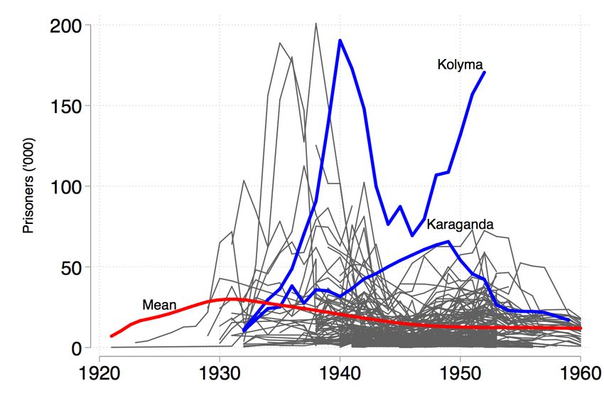
camps devoted to various economic activities such as forestry, mining, light and metal
manufacturing, or agriculture. While this dark episode in human history has been extensively
detailed by historians (e.g. Solzhenitsyn (1973), Applebaum (2012)) and is now in most
history textbooks, little economic research has been devoted to understanding its consequences
on the development of the countries’ involved.       We know from recent papers that the
population of cities where Gulag camps were located grew significantly faster from 1926 to
2010 than that of similar cities without camps (Mikhailova, 2012), and that Gulag districts
were associated with anti-communist voting during the 1990s (Kapelko and Markevich, 2014).

    We investigate the long-run consequences of the Gulag focusing on the development
impact of the forced displacement of enemies of the people. Enemies were the high-skilled,
educated elite (Miller and Smith, 2015), targeted by the authorities for they posed a threat
to the propaganda-dependant regime. For this reason we conjecture that their selection
into Gulags might have affected local economic outcomes via human capital channels. The
re-location of enemies was on a massive scale. One estimate suggests that 1.6 million (nearly
2.5% of the working population) had been arrested for counter-revolutionary violations
during the Great Terror of 1937 and 1938 alone (Kozlov, 2004). And as people often ended up
remaining in their Gulag’s town after the Gulag’s fall (Cohen, 2012), their forced re-location
might have persistent effects. The forced re-location of enemies can hence be seen as a
natural experiment that allows us to identify the long-run persistence of skills and its effect
on growth. In doing so we aim to contribute to the growing body of natural experiments in
macroeconomics (Fuchs-Schndeln and Hassan, 2016) and further our understanding of the
role of social structure in the uneven development outcomes we observe both across and
within countries.

    The heart of our empirical investigation is a dataset on Gulags from Memorial, an
organization in Moscow devoted to the memory of the Soviet Union’s totalitarian history.
This data provides information on the location, population, and economic activity of 474
camps from 1921 to 1960. Crucially, it provides information on the number of political

                                              2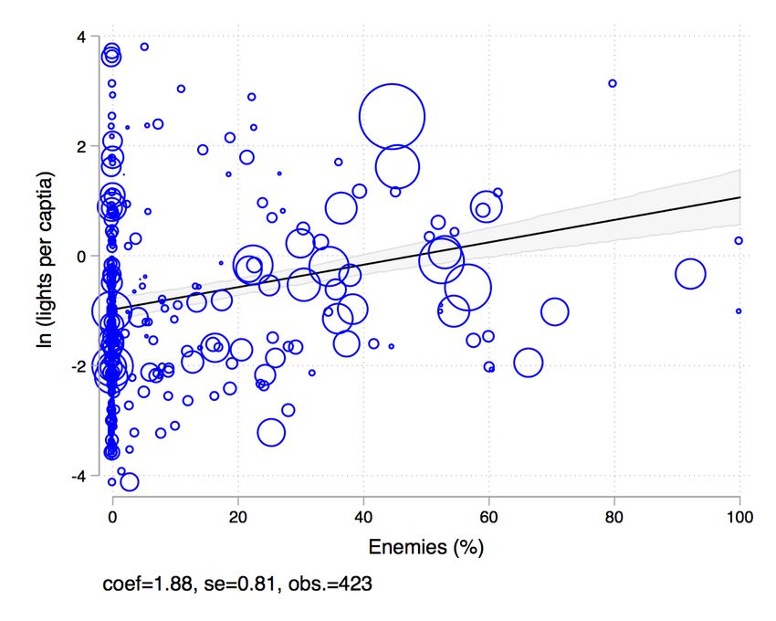
prisoners, or enemies, per camp and per year. This allows us to use the enemy share of the
camps’ population to capture the skill composition of the forced migration shocks, spread
across the Soviet Union like a chain of islands, i.e. the Gulag Archipelago (Solzhenitsyn,
1973). We then match spatially the camps’ locations with current economic activity and
education outcomes, using a household- and firm-level data as well as night light intensity.

       We first show that cities located within a 30km radius of Gulags which were populated
by a higher share of enemies are richer today, as proxied by lights per capita (Figure 1).1
We then show that in 2014 firms near those enemy-intensive Gulags are more productive
and pay higher wages to more educated workers. Moving from a town near a Gulag where
enemies accounted for 8% of prisoners, i.e. the average across camps, to one near a camp with
25% enemies, or a one standard-deviation increase from the mean (17 percentage points),
increases lights per capita by 15%, value added per employee by 22%, revenue per employee
by 26%, average wages by 14%, and the probability an employee is tertiary educated increases
by 10 percentage points. The latter result is robust to using education data from a 2010
household survey and the 1989 census. Our results point in the direction of a long-run
persistence of skills and a resulting positive effect on growth.2

       In providing evidence on the long-run effect of enemies our paper contributes to the
literature on long-run persistence, especially the subset that focuses on human capital and
growth.3 The role of human capital in growth is at the core of economics research but its
effect has been hard to identify.4
   1
     Lights per capita is a measure of prosperity akin to GDP per capita used by Pinkovskiy and Sala-i
Martin (2016) and Pinkovskiy (2017). The use of nighttime lights to measure economic activity in general
has been pioneered by Henderson et al. (2012).
   2
     It is important to note that the Gulag system is one of the most atrocious episode in recent history.
And while we find that inflows of enemies had positive long-run effects on local development, we do not
investigate the legacy of their mass removals on their home regions, for we do not have data on their origins.
   3
     The volume by Michalopoulos and Papaioannou (2017) and the literature review by Nunn (2009) cover
much of this new literature on the persistence of historical events. Examples include Dell (2010), who look
at the persistence of extractive institutions in Peru, Nunn (2008) who look at the long run effect of the slave
trade in African countries, Guiso et al. (2016) who look at the consequences of self-government in the Middle
Ages in Italian cities, and Grosfeld and Zhuravskaya (2015) who look at the legacies of three past empires
in Poland.
   4
     Barro and Lee (2010) suggest the cross-country rate-of-return to an additional year of schooling ranges

                                                      3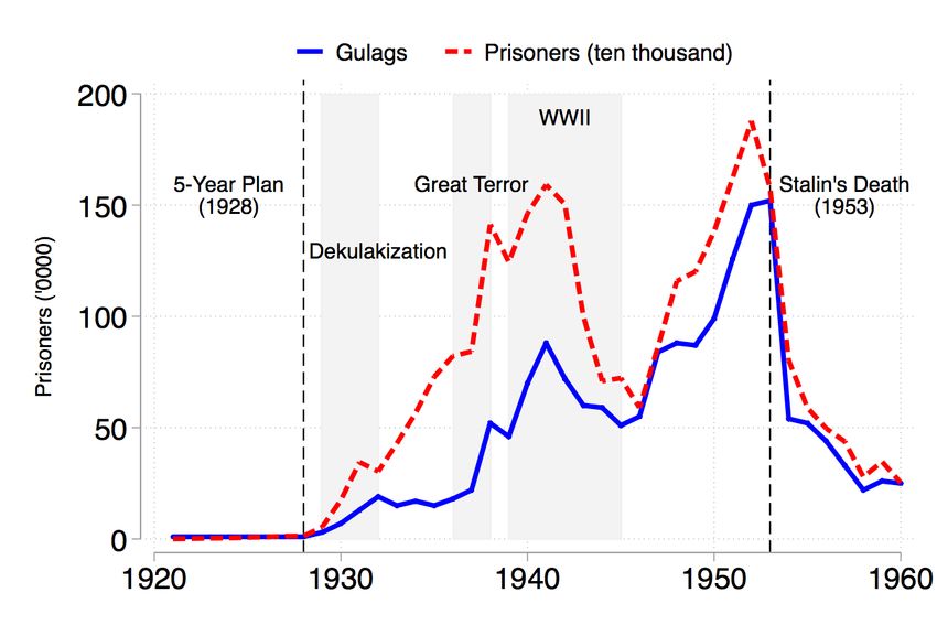
Figure 1. Enemies of the people (%) vs. lights per capita

Notes: The figure depicts the relationship between the share of enemies
across Gulags and the nightlight intensity within a radius of 30km of the
Gulags. Individual observations are weighted by camp prisoner population
(indicated by the size of the circles). The light intensity is calculated using
average population and light emission estimates within a radius of 30km
of the respective Gulag. The lights data is from the DMSP-OLS satellite
program and the grided population data is from SEDAC. The Gulag data
is from Memorial. See text for details.

                                      4
Many of the latest contributions rely on historical natural experiments of human capital
allocation across space to identify its effect on development. Easterly and Levine (2016)
for example document how the descendants of European colonizers are rich wherever they
are in the world as colonizers brought their human capital with them and this made their
host countries richer. Similarly, Rocha et al. (2017) shows that high-skilled immigrants
settled to particular regions of Brazil via a state-sponsored policy around 1900 have higher
levels of schooling and income per capita today. Droller (2018) shows that European settlers
raised literacy rates and helped industrialization in Argentinean counties. Hornung (2014)
shows that in the late 17th century Prussia, firms in areas receiving skilled Huguenots from
France experienced increased productivity. In Latin America (Valencia Caicedo, 2015) and
in Madagascar (Wietzke, 2015), human capital spillovers from missionary areas contributed
to superior education outcomes in former settler districts. Bazzi et al. (2016) also show that
farmers resettled by a policy experiment in Indonesia transfer their human capital and skills
and thus contribute to their host region development.5
A growing body of evidence thus suggests that migration has long-run effects as migrants
take their human capital with them and transfer it to their children and colleagues. The
mechanisms of transmission of social norms or skills over time are well understood and
documented. For example, Bisin and Verdier (2001) provide a model of intergenerational
cultural transmission where parents transmit their preferences to their offspring motivated
by a form of paternalistic altruism. Hvide and Oyer (2018) use dinner table human capital
from 5% to 12% across countries but these estimates are absent from the latest version of their work. More
fine-grained estimations include Gennaioli et al. (2013), Ciccone and Papaioannou (2009), and Squicciarini
and Voigtlander (2015) who present evidence that upper-tail knowledge was an important driver of city
growth during the first industrial revolution in France, mainly through increased productivity in industrial
technologies. Waldinger (2016) also provides evidence for the importance of upper-tail human capital in the
production of scientific knowledge using the dismissal of scientists in Nazi Germany as a natural experiment.
There is also a long-established literature highlighting the importance of human capital such as schooling in
accounting for productivity heterogeneity across firms (Abowd et al., 2005; Ilmakunnas et al., 2004; Fox and
Smeets, 2011).
5
It is worth mentioning that the effect migration on growth may not only be due to the selection of
high-skilled migrants but also to the fact that migration itself, especially forced migration, may give people
an incentive to invest in human capital. See for example Becker et al. (2018) who show that forced re-locations
within Poland had this effect on education attainment.
5to refer to industry knowledge learned through parents. Lindahl et al. (2015) document
persistence in educational attainments over four generations in Sweden, labelling this persistence
as dynastic human capital. Valencia Caicedo (2015) puts it as occupational persistence
and intergenerational knowledge transmission.6 Our paper further adds to this literature
by showing in additional results that the long-run effect of enemies on firm productivity
is strongest in local industries that date back to Gulag times. This suggests that the
intergenerational transmission of skills is strongest within specific industries and hence may
be linked to industry knowledge.
The rest of our paper is structured as follows. Section 2 provides the historical background,
Section 3 presents the data and empirical strategy, Section 4 our results and robustness checks
and finally Section 5 concludes.
2 HISTORICAL BACKGROUND
The Gulag was the Soviet system of corrective labor camps through which as many as 18
million people (the true figure remains unknown), from petty criminals to political exiles,
were re-located from 1918 to 1956. Around 474 camps were scattered across the Soviet
Union like a chain of islands (see Figure 2), what Aleksandr Solzhenitsyn called the Gulag
Archipelago.7 In this section we only scratch the surface on this dark episode in human
history. We’ll focus on the targeting of enemies of the people, often described as political
prisoners or counter revolutionaries.
6
Other examples include Grönqvist et al. (2016) who show that parents cognitive and non-cognitive
abilities are a strong predictor of their childrens education and labor market outcomes. Also Peisakhin
(2013) provides evidence on the role of families in transmitting historical political identities using the split
of Ukrainians between Austrian and Russian empires in the late 18th century.
7
The story of the massive and monstrous policy of the Gulag has been told and made famous by
(Solzhenitsyn, 1973) and more recently by Applebaum (2012). The Gulag Archipelago is now the most
cited work on the Soviet labor camp system and is common reading in Russian schools. It was a criminal
offence to read it until the late 1980s however.
6Figure 2. Location and size of Gulags
7
Notes: Source: Memorial.The idea of the Gulag and of the targeting of enemies of the people can be traced back to
Lenin. In a speech in 1917, he proclaimed that “All leaders of the Constitutional Democratic
Party, a party filled with enemies of the people, are hereby to be considered outlaws, and are
to be arrested immediately and brought before the revolutionary court... No mercy for these
enemies of the people, the enemies of socialism, the enemies of the working people! War
to the death against the rich and their hangers-on, the bourgeois intellectuals; war on the
rogues, the idlers and the rowdies!” (cited in Albert et al. (1999)). Applebaum (2012) notes
that by 1918 Lenin was already targeting aristocrats and merchants and having them locked
up in concentration camps outside major towns. She suggests that there were already as
many as 84 camps in 43 provinces in 1921, and these were specifically designed for these first
enemies of the people.
The mass arrests of enemies, that Lenin famously described as the faeces of the nation,
began in 1919. These enemies of the people were not precisely defined. They included
political opponents, journalists, bourgeois intellectuals, artists, professors, scientists, land-
owners, and speculators involved in trade. Class and education were often the key criteria
to be identified as an enemy. As Martin Latsis, a Soviet politician, wrote in 1920 “In the
interrogation do not seek evidence and proof that the person accused acted in word or deed
against Soviet power. The first questions should be: What is his class, what is his origin,
what is his education and upbringing? These are the questions which must determine the
fate of the accused.” (cited in Solzhenitsyn (1973)).
The targeting of the educated, but also the randomness of being labelled an enemy and
being sent away, can also be understood from the drawings by Baldaev (2010), a Gulag
guard.8 In one drawing depicting the secret police rounding up enemies to be deported, one
agent tells his colleagues: “We’ve been instructed to round up twelve enemies of the people.
With the engineer, the doctor woman and the old moron professor, we’ve only gotten ten.
Take any two people from the apartments on the first floor, whoever you can get - workers
8
The drawings by Baldaev (2010) provide a vivid illustration of the atrocities of the re-location process
and the camps.
8or kolkhozniks (farmers) - it doesn’t matter. We just need twelve people in all. That’s an
order. Off you go...”.9
In the 1920s Stalin started pushing for the fast industrialization of the Soviet Union, and
this involved the mass re-locations of enemies and other prisoners to an expanding number of
Gulags (see Figure 3). Article 58 of the Russian Penal Code put into force in 1927 formalized
the criminality of enemies, defining a counter-revolutionary action as “any action aimed at
overthrowing, undermining or weakening of the power of workers’ and peasants’ Soviets and
governments of the USSR and Soviet and autonomous republics, or at the undermining or
weakening of the external security of the USSR and main economical, political and national
achievements of the proletarial revolution.” The 1928 Five-Year Plan on the use of forced
labor explicitly stated that convicts receiving a sentence in prison exceeding 3 years, as most
enemies did, should be allocated to labor camps.
According to Hosford et al. (2006), the campaign against enemies of the people that
followed occurred through three major waves. The first was the deportations and executions
of millions of Kulaks, or dekulakization, from 1929 to 1932. The Kulaks were the well-off
peasants that used hired labor, or owned mills or other processing equipment. In reality
any peasant who sold his surplus goods on the market could be classified as a Kulak. The
second major wave of arrests is known as the Kirov flood, triggered by the assassination of
Sergei Kirov, the head of the Communist Party in Leningrad, in 1934. In the months that
followed his death, around 40,000 residents of Leningrad were rounded up. The third episode
is the Great Terror of 1937-1938, when 1.5 million enemies were arrested, and half of them
executed (Harrison, 2008). Hosford et al. (2006) cites a propaganda doggerel written in 1937
9
Eugenia Ginzburg, a teacher and member of the Communist party, sent to the Gulag for
counter-revolutionary activity in 1937, also describes the various type of enemies who had been sent to
camps in her memoir about Gulag survival, Journey into the Whirlwind (Ginzburg, 2002). She recounts how
once in a camp hospital in Siberia she found herself among her own: “I had seen no men of this sort; our
sort - the intellectuals; the country’s former establishment - since transit camp... The men here were like us.
Here was Nathan Steinberger; a German Communist from Berlin. Next to him was Trushnov; a professor
of language and literature from somewhere along the Volga; and over there by the window lay Arutyunyan;
a former civil engineer from Leningrad... By some sixth sense they immediately divined that I was one of
them and’ rewarded me with warm, friendly; interested glances.” (cited in Shatz (1984)).
9by Demian Bedny, a poet, dehumanizing enemies and supposed to serve as an apologia for
the Great Terror: “How disgraceful the sight of enemies among us! Shame to the mothers
that gave birth To these vicious dogs of unprecedented foulness! ”
The Gulag played a central role in the Soviet economy, mining one-third of all the
Soviet Union’s gold, and much of its coal and timber. The camps were of various types,
from prisons surrounded with barbed wire to unguarded towns in remote locations, and
were often devoted to a particular economic activity, from mining to manufacturing and
agriculture. As Hosford et al. (2006) writes, “the GULAG participated in every sector of
the Soviet economy, including mining, highway and rail construction, arms and chemical
factories, electricity plants, fish canning, airport construction, apartment construction and
sewage systems. Among the items prisoners produced were missiles, car parts, leather goods,
furniture, textiles, glass cups, lamps, candles, locks, buttons and even toys.”. The system
expanded until Stalin’s death in 1953, when the camps total population reached 1,727,970,
after which the system slowly came to an end.
One example of such camp was KarLag, immortalised by Solzhenitsyn’s One Day in the
Life of Ivan Denisovich 10 . Karlag was one the largest labor camps of the Soviet Union (see
Figure 3), located near Karaganda in the sparsely populated steppe of Kazakhstan. The
choice of KarLag’s location was mainly determined by large coal deposits and an abundance
of iron and nonferrous metals. The steppes surrounding Karaganda were transformed into a
centre for metallurgical industry running on coal and labor (Harris, 1945). This required the
mass relocation of thousands of workers. These were mostly involved in resource extraction
10
It is worth emphasizing again that, as detailed in One Day in the Life of Ivan Denisovich, living
conditions in the camps were a traumatising experience. Prisoners often were forced into harsh physical
labor while living in overcrowded camps with little food, insufficient clothing, and poor hygiene. Mortality
rates were around five times higher than on average in the Soviet Union Khlevniuk (2004) and Blyth (1995)
estimated the number of deaths in camps to be between 9.7 and 16.7 million. A memo from a procurator of
the Soviet Union to the chief of the People’s Commissariat for Internal Affairs in 1938 stated that “Among
the prisoners there are some so ragged and liceridden that they pose a sanitary danger to the rest. These
prisoners have deteriorated to the point of losing any resemblance to human beings. Lacking food . . . they
collect orts [refuse] and, according to some prisoners, eat rats and dogs.” (Brent, 2008). Khlevniuk (2004)
also notes that there were corrosive and violent measures to keep inmates in check and camps were told not
to spare bullets when inmates attempted to escape.
10Figure 3. The evolution of the Gulag
Notes: The top figure shows the number of Gulag camps and the total
number of prisoners while the bottom one shows the number of prisoners in
each camp. Each grey line is the prisoner population of one camp. The red
line is the yearly average. Source: Memorial.
11and processing but some were agricultural scientists publishing articles on fertilisation in the
Kazakh steppe (Shaimuhanov and Shaimuhanova, 1997). One estimate suggests that over
50% of Karlag’s population were enemies (Memorial, 2016). Karaganda continued growing
for several decades after KarLag’s closure, reaching a population above half a million within
40 years of its creation.
Table 1: Share of prisoners by education
Education Gulag Enemies∗ Pop. Pop.
1937 (1927-1953) 1937 1926
Tertiary (%) 1.0 4.6 0.6 -
Secondary (%) 8.9 13.0 4.3 -
Elementary (%) 49.3 56.0 38.3 -
Semi literate (%) 32.4 - - -
Illiterate (%) 8.4 26.0 39.0 61.0
Notes: *Author’s calculation based on individual-level data from
Memorial. Other data from J. Arch Getty (1993) and 1926 Census.
The legacy of the Gulag is not yet fully understood. We do know that after the fall of
the Gulag prisoners often had to settle down and continue working at the same industrial
projects as outside options were heavily limited (Cohen, 2012). We also know that a number
of major industrial cities in Russia and other ex-Soviet countries were originally camps built
by prisoners and run by ex-prisoners. And finally, we know that cities where Gulag camps
were located grew significantly faster than similar cities without camps from 1926 to 2010
(Mikhailova, 2012).11
In this paper we stress the importance of the selection of highly educated enemies into
the Gulag to explain its economic legacy. Enemies, or educated dissidents, amounted to
around one third of the Gulag population (J. Arch Getty, 1993). What this elite targeting
implied was a higher education level on average in camps than in society as a whole. Table
1 compares the education levels of the Gulag population to that of the Soviet Union as
a whole in 1926 and 1937. It suggests that the share of people with school achievement
11
Mikhailova (2012) argues that the Gulag had a permanent effect on the economy’s spatial equilibrium,
whereas WWII evacuations and enterprise relocations did not.
12above secondary was twice as high in Gulags, at around 10% in 1937. And only 8.4% of
the Gulag prisoners were illiterate compared to as much as 39% of the Soviet population.
Individual-level data from Memorial on enemies suggest the latter were even more educated,
with as much as 17.6% of them having at least a secondary education. In the rest of our
paper we investigate whether the skill composition of camps captured by the share of enemies
across camps may have led to positive education and growth outcomes.
3 DATA AND EMPIRICAL STRATEGY
The heart of our empirical investigation is a dataset on Gulags from Memorial, an organization
in Moscow devoted to the memory of the Soviet Union’s totalitarian history. This data
provides information on the location, population, and economic activity of 474 camps from
1921 to 1960. Crucially, it provides information on the number of political prisoners, or
enemies, per camp and per year, among other camp descriptors available on camp-specific
webpages.12
Our variable of interest is the enemy share of the Gulag’s prisoner population. The data
provides yearly observations on total prisoners and enemies for the Gulag years but as we
are interested in the geographic variation in enemies across Gulags, we take the median
number of enemies and divide it by the median number of prisoners by camp. This gives
us an indication of the Gulag’s skill composition during the whole period and is not driven
by outlier years. It is also not affected by missing observations, i.e. camp-years with no
information on enemies. We thus define our variable of interest, varying across Gulags g, as:
Median number of Enemiesg
Enemies(%)g ≡ Median number of Prisonersg
12
The historical Memorial data on Gulags is also available from Tatiana Mikhailova online but this version
does not contain information on enemies. While the memorial data does not provide information on the
ethnicity of the prisoners, we know from J. Arch Getty (1993) that the Gulag population was as diverse
ethnically as that of the Soviet Union at large. In 1939 63% of prisoners were Russians, 13.8% Ukrainians
while Belorussians, Tatars, Uzbeks, Jews, Germans, Kazakhs, Poles, Georgians, Armenians, Turkmen,
Latvians, Finns accounted for the rest. If any ethnic group was at all over represented in camps, it was
Russians.
13Figure 4. The distribution of enemy shares across camps
Notes: The first column, including Gulags with zero enemies, adds
up to 314 camps. Source: Memorial.
The distribution of enemies (%) across Gulags is depicted in Figure 4. Out of 423 camps,
314 have less than 5% enemies among their prisoner population. There is, however, a large
number of camps with a large share of enemies. The average share is 8% and the standard
deviation is 17 percentage points.
According to the aggregate data used in J. Arch Getty (1993) and shown in Figure 5,
enemies, labeled here as counterrevolutionaries, amounted to around one third of the Gulag
population. Our camp-level data, shown in the bottom panel of Figure 5, gives us similar
yearly aggregated prisoner numbers. While we do not have sufficient yearly observation to
estimate the share of enemies in each year, we do match closely the aggregate share for the
years for which we have enemy numbers. This confirms that the data we use on the shares
of enemies across Gulags, obtained using the years for which data is available, is in line with
aggregate figures from previous studies.
For our analysis we will test the robustness of our results to two samples of Gulags.
14Figure 5. The enemy share of Gulag prisoners
Notes: The top panel is from J. Arch Getty (1993). The bottom panel graphs
our estimates from Memorial data. The number of enemies is available for a
large number of camps for the years 1938/1939 and 1942/1943 so we focus on
this period to estimate aggregate numbers. For most camps we only have data
on enemies for one of the two years in these two periods. We use numbers from
the first year if available and numbers from the second year otherwise.
15The baseline sample of 423 Gulags include all Gulags for which we have information on the
number of enemies and total prisoners. The robustness sample includes a subset of 238
Gulags that existed for at least 2 years. This subset of camps has more information on the
number of enemies across years and hence will allow us to check if our results are sensitive
to the quality of our enemy data. Also, the reduced sample might be a less noisy a measure
of enemy exposure as short-lived camps might not have the same persistence effects. We
include estimates based on these two samples throughout our results section.
To examine the long-run effect of enemies on growth we merge spatially the camps’
locations to information on economic activity and education from three datasets.
First we proxy for local GDP per capita using satellite data on night light intensity
collected by the DMSP-OLS satellite program and made available by the Earth Observation
Group and the NOAA National Geophysical Data Center13 , which we combine with data on
population from the grided population of the world from SEDAC.14 Data on light intensity
and population is for 2010. Lights per capita are a good proxy for economic activity as
consumption in the evening requires lights, and hence light usage per person increases with
income (Henderson et al., 2012). Lights per capita have been used as a measure of prosperity
akin to GDP per capita by Pinkovskiy and Sala-i Martin (2016) and Pinkovskiy (2017).
The use of nighttime lights to measure economic activity in general has been pioneered by
Henderson et al. (2012). Figure 6 illustrates how our spatial matching of night lights and
camp locations allows us to check whether enemies are an important predictor of lights per
capita across cities. It shows how in the far east of Russia for example, Gulags, whether
they hosted enemies or not, are more often located near economic activity.
The other two datasets we use are firm and household surveys conducted by the European
Bank for Reconstruction and Development (EBRD) and the World Bank. The firm-level
13
Light intensity is measured on a scale between 0 and 63.
14
The Gridded Population of the World (GPW) dataset is constructed using national censuses and
maintained by the Socioeconomic Data and Applications Center (SEDAC) at the Center for International
Earth Science Information Network at the Earth Institute at Columbia University.
16Figure 6. Matching Gulag locations with night lights
survey is the Business Environment and Enterprise Performance Survey (BEEPS), which is a
representative sample of an economy’s private sector and is based on face-to-face interviews
with managers. We use data from the fifth round of BEEPS in 2011-2014 which covers
almost 16,000 enterprises in 30 countries, including 4,220 enterprises in 37 regions in Russia.
It includes questions on a broad range of business environment topics including sales, costs,
and employees. The household survey is the second Life in Transition survey (LiTS 2)
which surveyed almost 39,000 households in 34 countries in 2010 to assess public attitudes,
well-being and the impacts of economic and political change. We use BEEPS data to measure
firm productivity as sales per employee or value-added per employee, average wages, and
workforce education. We use LiTS data to measure household’s education and corroborate
the firm-level data. We thus examine the long-run effect of enemies on development by
linking the location of Gulags to firms in 2014 and households in 2010 in all countries of
the former Soviet Union. The geographic coverage of the firms and households which we
were able to link to the location of Gulags (radius of 30km) is summarized in Table 2. The
descriptives of the main outcome variables on education are summarized in Table 3.
17Table 2: Gulags, firms, and households
Number of Observations Enemies (%)
Gulags Firms Households Mean SD
(1) (2) (3) (4) (5)
Azerbaijan 4 248 240 0 0
Georgia 1 176 300 0 0
Kazakhstan 17 270 200 7 15
Kyrgyzstan 2 152 40 0 0
Russia 374 2397 398 8 17
Tajikistan 3 117 20 0 0
Ukraine 16 185 166 0 0
Uzbekistan 2 208 80 6 12
Sum 423 3753 1444
Average 8 17
Notes: Gulags with insufficient information on location or economic activity
have been excluded from the analysis. Only firms and households within a
radius of 30km of a camp have been included in our analysis.
Table 3: Descriptive Statistics on Education
variable mean sd max min obs.
Years of education (Firm Level) 12.37 2.18 20 0 985
>13 years education (Firm Level) 0.29 0.45 1 0 985
Tertiary education (Household Level) 0.33 0.46 1 0 824
Primary Education 1926 (Census) 0.35 0.14 0.71 0.04 92
Tertiary Education 1989 (Census) 0.09 0.03 0.21 0.04 92
Source: Calculations based on BEEPS, LiTS and Census data
18Before investigating the legacy of the enemies of the people it is important to ask whether
enemies were systematically sent to some specific regions or industries. Indeed enemies
might have been allocated to more productive regions with better soil, or to skill-intensive or
capital-intensive activities. They also might have been sent to the larger camps benefitting
from agglomeration economies and higher productivity.
After going through the historical narrative of the Gulag, provided in particular by the
books of Solzhenitsyn (1973) and Applebaum (2012), to check if there was any systematic
bias in the allocation of enemies, we found no indication of such a system. The deportation
process is rather described as rushed and disorganized, with random arrests and train
packing. Both authors also suggest that political prisoners were often not allowed to be
involved in skilled labor and were nearly always mixed with the non-political offenders doing
unskilled work. In fact, according to an official decree released on the 7th of April 1930 by
the Council of People’s Commissars, prisoners convicted of counter-revolutionary activities
were not allowed to occupy any administrative-economic position.
We nonetheless check whether Gulags with enemies of the people differ statistically from
other Gulags across geographic or industrial characteristics. The relevant summary statistics
are in Table 4. As we explain above, we use two samples of Gulags. The All Gulags sample
includes the 423 camps for which we have at least one year of enemy data. The > 2 years
sample includes only the Gulags that were active for at least 2 years for which we have
more years of data. Across economic activities, we find enemy Gulags more likely to focus
on agriculture and the food industry. Interestingly, enemy Gulags are less likely to focus
on research or energy. Across resource extraction sectors we find no statistical difference
between enemy and non-enemy Gulags except for gold, which is more prevalent in enemy
Gulags. Across climate and land characteristics, we find enemy Gulags to be located further
East on average, to be colder and drier in winter, and to have inferior soil (higher numbers for
workability and rooting). Enemy Gulags are also more likely to be further away from densely
populated urban areas. To sum up, enemies were more likely to be sent to less populated
19locations with worse climatic conditions and be employed in sectors such as agriculture and
food processing. These differences however do not point to a systematic allocation of enemies
to camp location or industries that may be drivers of prosperity and firm productivity today.
We nonetheless control for these sources of variation in our regressions so that we identify
as precisely as possible the effect of enemies’ skills.
In Table 5 we check if the share of enemies in a camp is conditionally correlated with
any of these characteristics. We run a regressions with all variables included on the right at
the same time to estimate conditional relationships:
Enemies(%)g = c + Xg0 γ + eg
We run both a standard cross-section OLS with Conley standard errors (30km) and a
weighted regression in which individual observations are weighted by the median number
of prisoners by camp. We find that conditional on other variables, the share of enemies
increases significantly as we move north and away from urban centers. We also find the
share of enemies to be higher in Gulags with a food industry and lower in Gulags with
a research industry. These slight differences across Gulags do not suggest any type of
systematic allocation of enemies that might affect their legacy. The allocation of enemies
across Gulags can hence be thought of as a natural experiment that allows us to identify the
effect of skill persistence on growth.
To examine the differences in lights per capita across 30km-radius areas around Gulags
with different shares of enemies, we start by estimating the following model at the Gulag
level:
(1) Lightsg = β1 Enemies(%)g + Xg0 δ + g ,
where Lightsg is night light intensity within a 30km radius around Gulag g, Enemies(%)g
20Table 4: Gulag characteristics for the period 1927-1953
All Gulags p-value Gulags (> 2 years) p-value
No Enemies Enemies (1)=(2) No Enemies Enemies (4)=(5)
(1) (2) (3) (4) (5) (6)
Enemies (’000) 0 3.8 0.00 0 4.3 0.00
Share Enemies (%) 0 23 0.00 0 24 0.00
Population
Prisoners (’000) 8 12 0.01 12 14 0.29
Population Den. 25 13 0.01 23 12 0.00
Urbanisation (%) 25 19 0.04 23 19 0.05
Climate and Land
Longitude 64 79 0.00 66 78 0.03
Latitude 55 56 0.22 55 56 0.54
Elevation 269 305 0.38 255 305 0.22
Ruggedness 97 106 0.47 90 110 0.25
Rooting 1.7 2.4 0.00 1.78 2.23 0.05
Workability 1.7 2.3 0.00 1.81 2.25 0.05
Precip. (Jan.) 30 26 0.00 29 26 0.03
Precip. (July) 75 75 0.78 75 76 0.63
Temp. (Jan.) -14 -18 0.00 -15 -18 0.00
Temp. (July) 18 17 0.08 17 17 0.26
Resource Extraction
Calciumph. (%) 1 2 0.43 1 3 0.28
Coal (%) 4 6 0.44 7 7 0.92
Gold (%) 2 6 0.05 3 8 0.06
Iron (%) 1 1 0.40 1 2 0.52
Stone (%) 11 9 0.44 16 9 0.09
Economic Activity
Agriculture (%) 14 38 0.00 21 43 0.00
Forestry (%) 28 45 0.00 45 49 0.49
Infrastructure (%) 58 66 0.09 60 67 0.23
Metal (%) 4 6 0.20 5 8 0.34
Material (%) 18 24 0.09 29 27 0.62
Mechanical (%) 3 6 0.15 6 7 0.67
Food Industry (%) 7 20 0.00 11 25 0.01
Energy (%) 7 6 0.86 6 5 0.68
Research (%) 5 3 0.36 6 3 0.42
Services (%) 13 18 0.16 19 20 0.90
Number of Gulags 284 139 124 114
Note: Column 3 and 6 display the p-value of a mean comparison test of columns 1 and 2 and 4 and 5
respectively. Note that 34 Gulags are located in Moscow. Excluding these does not significantly affect our
main conclusions.
21Table 5: The correlates of enemies
Dependent variable: Share of enemies among prisoners
All Gulags Gulags (> 2 years)
Conley50km Weighted Conley50km Weighted
(1) (2) (3) (4)
Prisoners (’000) 0.001∗ 0.000 0.001 -0.000
(0.001) (0.000) (0.001) (0.000)
Population Den. 0.000 0.001 0.001 0.001
(0.000) (0.001) (0.001) (0.001)
Urbanisation -0.115∗∗ -0.223∗∗ -0.184∗ -0.329∗∗
(0.056) (0.104) (0.107) (0.162)
Longitude 0.001 0.000 0.000 -0.000
(0.000) (0.001) (0.000) (0.001)
Latitude 0.007∗∗ 0.007 0.008∗∗ 0.009
(0.003) (0.004) (0.003) (0.006)
Elevation -0.000 -0.000 -0.000 -0.000
(0.000) (0.000) (0.000) (0.000)
Ruggedness 0.000 0.000 0.000 0.000
(0.000) (0.000) (0.000) (0.000)
Rooting -0.014 -0.169 -0.079 -0.270
(0.100) (0.167) (0.148) (0.167)
Workability 0.008 0.167 0.072 0.262
(0.102) (0.167) (0.150) (0.167)
Precip. (Jan.) -0.000 -0.001 -0.001 -0.004
(0.001) (0.001) (0.001) (0.003)
Precip. (July) -0.000 -0.001 -0.000 -0.001∗
(0.000) (0.001) (0.000) (0.001)
Temp. (Jan.) -0.002 -0.001 -0.003 0.000
(0.002) (0.004) (0.003) (0.006)
Temp. (July) 0.008∗∗ 0.006 0.009∗∗ 0.005
(0.004) (0.006) (0.004) (0.008)
Calciumph. -0.114 -0.018 -0.021 0.052
(0.070) (0.093) (0.080) (0.120)
Coal -0.019 0.012 -0.034 -0.030
(0.034) (0.062) (0.041) (0.069)
Gold 0.013 0.027 0.023 0.046
(0.034) (0.078) (0.048) (0.085)
Iron -0.028 -0.086 -0.030 -0.116
(0.050) (0.087) (0.062) (0.103)
Stone -0.018 -0.082∗∗∗ -0.033 -0.109∗∗
(0.021) (0.031) (0.030) (0.044)
Agriculture 0.022 0.037 0.030 0.025
(0.020) (0.032) (0.026) (0.038)
Forestry 0.016 0.056∗ 0.004 0.044
(0.020) (0.033) (0.030) (0.039)
Infrastructure 0.013 0.034 0.010 0.034
(0.014) (0.026) (0.022) (0.036)
Metal 0.034 0.083 0.028 0.090
(0.035) (0.050) (0.043) (0.063)
Mechanical 0.025 0.010 0.012 0.012
(0.040) (0.044) (0.049) (0.050)
Material -0.006 -0.008 -0.027 -0.018
(0.020) (0.035) (0.025) (0.043)
Food Industry 0.077∗∗ 0.070∗ 0.103∗∗∗ 0.075∗
(0.031) (0.039) (0.035) (0.043)
Energy -0.026 -0.043 -0.039 -0.064
(0.022) (0.040) (0.040) (0.057)
Research -0.048∗∗ -0.088∗∗ -0.051 -0.072∗
(0.023) (0.035) (0.040) (0.042)
Service 0.027 0.020 0.033 0.007
(0.028) (0.039) (0.043) (0.051)
N 423 423 238 238
R-sq 0.30 0.26 0.40 0.30
Note: Conley standard errors are in parentheses : *** pis the share of enemies among all prisoners in Gulag g; and Xg is a set of control variables
which include fixed effects capturing Gulags’ economic activities, the number of prisoners in
the Gulag, as well as location specific variables, i.e. country fixed effects, latitude, longitude,
ruggedness, and elevation. We account for spatial correlation across nearby Gulags using
Conley standard errors for g .
To examine the differences in performance and education outcomes across firms and
households near Gulags with different shares of enemies, we estimate the following model at
the firm or household level:
(2) Yi = β1 Enemies(%)i + Xi0 δ + i ,
where Yi is a measure of labor productivity or human capital reported by firm or
household i, Enemies(%)i is the share of enemies in Gulags within 30km of firm or household
i; and Xi includes location specific controls, i.e. country fixed effects, latitude, longitude,
ruggedness, elevation, as well as fixed effects capturing the firms’ industries or the occupation
of household heads as well as gender, age, and age squared. It also includes the number of
prisoners in Gulags within 30km of firm or household i, and fixed effects for the Gulags’
economic activities. We cluster the error term, i by geographic clusters of Gulag exposure.
To measure labor productivity we use the firms’ value added per employee but also a
measure of revenues per employee which allows us to include the entire sample of firms, as
some firms drop out when we compute value added due to missing data on inputs. It is
worth noting that revenues per employee is a common metric used by investors and industry
analysts to understand how efficiently a firm uses its employees. We also compute the firms’
average wages by dividing total labor costs by the number of employees. Finally the firm
data also contains information on the average years of education of production employees
which allows us to measure education in years and also as a tertiary education dummy,
which we define as equal to 1 if education years is above 13, and zero otherwise. We also
23use household survey data on the tertiary education of household heads to check for the
robustness of the effect of enemies on education outcomes.
4 RESULTS
4.1 BASELINE
The estimates of the effect of enemies (%) on lights per capita are in Table 6. In our
benchmark specification which includes all controls and fixed effects (Panel A, column 2),
we find that a one standard deviation increase in Enemies (%) increases lights per capita
by 15% (e.819∗.17 ). Results are twice as big in a specification without geographic controls or
Gulag activity indicators (column 1). In column (3) we focus only on Russia, where almost
90% of Gulags were located, and find similar results. Results in columns 4 to 6 replicate
columns 1 to 3 but focusing on our restrained sample of Gulags, i.e. those active for more
than two years. While the number of observations falls by almost half, the results are of the
same magnitude as in the full-Gulag sample specifications. In the bottom panel (Panel B),
we include robustness checks where we measure enemy exposure using a dummy variable
equal to one if enemies were sent to that Gulag, and zero otherwise, instead of the actual
share of enemies. The coefficients in these specifications are positive though not statistically
significant at the 90% level. Nonetheless they are in line with our baseline. Column (2) in
Panel B suggests that in Gulags with enemies light intensity per capita is 14% higher. It is
also worth noting that Gulags that did not survive, i.e. those that became pitch black on
the lights map, have a lower share of enemies.
Our estimates of the effect of Enemies (%) on firm-level revenues per employee, value
added per employee, average wages, and employee education are in Tables 7, 8, 9, 10, and
11. We find that a one standard deviation increase in enemy share, i.e. a 17 percentage
point increase, increases revenues per employee by 26%, value added per employee by 22%,
24Table 6: Dependent Variable: Lights per capita (ln)
Panel A: Share of Enemies of the People
All Gulags Gulags (>2 years)
(1) (2) (3) (4) (5) (6)
∗∗∗ ∗∗ ∗∗ ∗∗ ∗
Enemies (%) 1.559 0.819 0.925 1.252 0.728 0.925∗
(0.470) (0.402) (0.411) (0.501) (0.437) (0.506)
N 423 423 386 238 238 217
R-sq 0.34 0.44 0.41 0.31 0.43 0.40
Panel B: Dummy Variable
All Gulags Gulags (>2 years)
(1) (2) (3) (4) (5) (6)
∗
Enemies (=1) 0.296 0.141 0.163 0.090 0.030 0.079
(0.178) (0.162) (0.171) (0.210) (0.189) (0.199)
N 423 423 386 238 238 217
R-sq 0.33 0.43 0.41 0.29 0.42 0.39
Total prisoners Y Y Y Y Y Y
Country FE Y Y Y Y Y Y
Geography N Y Y N Y Y
Gulag activity N Y Y N Y Y
Conley standard errors in parenthesis, and * stands for statistical significance at the 10%
level, ** at the 5% level and *** at the 1% percent level. In column 1-3 we use the full
sample of Gulags. In column 4-6 we use only Gulags which remained active for more than 2
years. In column 1 and 4 we present the results with country fixed effects as well as the the
total number of prisoners. In column 2 and 5 we control for additional geographical variables
as well as dummies indicating the main economic activities of Gulags. In column 3 and 6 we
focus only on Russia, using the full-control specification of column 2 and 5.
25average wages by 14%, years of education by 3 months, and the probability to have a tertiary
education by 10 percentage points. The statistical significance of these effects is robust
across specifications except for the wage regressions, where we obtain less precise though
still positive estimates.
In Table 12 we confirm the effect of enemies on the areas’ share of tertiary educated
people using household survey data from LiTS. Here the industry dummies are occupation
dummies but the specification is similar otherwise. We find robust positive effects of enemies
on the probability of a nearby household’s head to have a tertiary education. In our baseline,
a 17 percentage point increase in enemy share increases the probability of being tertiary
educated by 6 percentage points. Focusing only on Russia suggests a larger effect. Here a
similar increase in enemies increases the the probability of being tertiary educated by 13.5
percentage points.
These results suggest that areas around more enemy-intensive Gulags are richer today.
They have more intense night lights per capita, here used as a proxy for GDP per capita, and
local firms have higher levels of labor productivity and pay higher wages to more educated
workers. This is in line with our conjecture that the skills transferred by forcedly displaced
enemies do indeed matter in explaining prosperity across regions of the ex-Soviet Union.
4.2 ROBUSTNESS TO CENSUS DATA
As a further robustness check on the legacy of enemies of the people on the areas average
education levels, we estimate the effects of enemies on the share of tertiary educated in 1989,
using data from the last Soviet census at the regional level, i.e. across 92 administrative units
knows as oblasts. To aggregate our enemy data at the oblast level we use enemies as a share
of the oblast’s 1926 population (before most of the forced resettlements), to which we add
the camp prisoner population. This allows us to measure how big a shock the enemies’
relocation was relative to the initial oblast’s population as well as the camp’s populations.
26Table 7: Dependent Variable: Revenues per employee (ln)
Panel A: Share of Enemies of the People
All Gulags Gulags (>2 years)
(1) (2) (3) (4) (5) (6)
Enemies (%) 0.990∗∗ 1.373∗∗∗ 1.864∗∗∗ 1.117∗∗ 1.824∗∗∗ 2.189∗∗∗
(0.471) (0.407) (0.465) (0.486) (0.419) (0.487)
N 2645 2645 1735 2323 2323 1614
R-sq 0.66 0.67 0.16 0.62 0.62 0.16
Panel B: Dummy Variable
All Gulags Gulags (>2 years)
(1) (2) (3) (4) (5) (6)
Enemies (=1) 0.355∗∗∗ 0.308∗∗∗ 0.305∗∗∗ 0.407∗∗∗ 0.357∗∗∗ 0.316∗∗∗
(0.098) (0.069) (0.076) (0.103) (0.066) (0.080)
N 2645 2645 1735 2323 2323 1614
R-sq 0.67 0.67 0.16 0.62 0.63 0.16
Total prisoners Y Y Y Y Y Y
Country FE Y Y Y Y Y Y
Industry FE Y Y Y Y Y Y
Geography N Y Y N Y Y
Gulag activity N Y Y N Y Y
Standard errors in parenthesis clustered by geographic exposure to enemies, and * stands
for statistical significance at the 10% level, ** at the 5% level and *** at the 1% percent
level. In column 1-3 we use the full sample of Gulags. In column 4-6 we use only Gulags
which remained active for more than 2 years. In column 1 and 4 we present the results with
country and industry fixed effects as well as the the number of prisoners (ln). In column
2 and 5 we control for additional geographical variables as well as dummies indicating the
main economic activities of Gulags. In column 3 and 6 we focus only on Russia, using the
full-control specification of column 2 and 5.
27Table 8: Dependent Variable: Value Added per employee (ln)
Panel A: Share of Enemies of the People
All Gulags Gulags (>2 years)
(1) (2) (3) (4) (5) (6)
∗∗ ∗∗∗ ∗∗∗
Enemies (%) 0.598 1.176 1.633 0.656 1.560 1.985∗∗∗
(0.444) (0.472) (0.542) (0.460) (0.513) (0.557)
N 1848 1848 1337 1657 1657 1255
R-sq 0.67 0.67 0.25 0.61 0.62 0.26
Panel B: Dummy Variable
All Gulags Gulags (>2 years)
(1) (2) (3) (4) (5) (6)
∗∗∗ ∗∗ ∗∗ ∗∗∗ ∗∗∗
Enemies (=1) 0.296 0.222 0.240 0.330 0.254 0.249∗∗
(0.110) (0.096) (0.100) (0.118) (0.098) (0.104)
N 1848 1848 1337 1657 1657 1255
R-sq 0.67 0.67 0.25 0.62 0.62 0.25
Total prisoners Y Y Y Y Y Y
Country FE Y Y Y Y Y Y
Industry FE Y Y Y Y Y Y
Geography N Y Y N Y Y
Gulag activity N Y Y N Y Y
Standard errors in parenthesis clustered by geographic exposure to enemies, and * stands
for statistical significance at the 10% level, ** at the 5% level and *** at the 1% percent
level. In column 1-3 we use the full sample of Gulags. In column 4-6 we use only Gulags
which remained active for more than 2 years. In column 1 and 4 we present the results with
country and industry fixed effects as well as the the number of prisoners (ln). In column
2 and 5 we control for additional geographical variables as well as dummies indicating the
main economic activities of Gulags. In column 3 and 6 we focus only on Russia, using the
full-control specification of column 2 and 5.
28Table 9: Dependent Variable: Average wages (ln)
Panel A: Share of Enemies of the People
All Gulags Gulags (>2 years)
(1) (2) (3) (4) (5) (6)
∗ ∗
Enemies (%) 0.236 0.762 0.960 0.439 0.600 0.699
(0.480) (0.422) (0.522) (0.621) (0.452) (0.574)
N 2588 2588 1531 1723 1723 1141
R-sq 0.74 0.75 0.09 0.64 0.65 0.10
Panel B: Dummy Variable
All Gulags Gulags (>2 years)
(1) (2) (3) (4) (5) (6)
∗ ∗∗
Enemies (=1) 0.233 0.087 0.150 0.270 0.106 0.103
(0.120) (0.090) (0.107) (0.137) (0.099) (0.126)
N 2588 2588 1531 1723 1723 1141
R-sq 0.74 0.75 0.09 0.64 0.65 0.10
Total prisoners Y Y Y Y Y Y
Country FE Y Y Y Y Y Y
Industry FE Y Y Y Y Y Y
Geography N Y Y N Y Y
Gulag activity N Y Y N Y Y
Standard errors in parenthesis clustered by geographic exposure to enemies, and * stands
for statistical significance at the 10% level, ** at the 5% level and *** at the 1% percent
level. In column 1-3 we use the full sample of Gulags. In column 4-6 we use only Gulags
which remained active for more than 2 years. In column 1 and 4 we present the results with
country and industry fixed effects as well as the the number of prisoners (ln)]. In column
2 and 5 we control for additional geographical variables as well as dummies indicating the
main economic activities of Gulags. In column 3 and 6 we focus only on Russia, using the
full-control specification of column 2 and 5.
29Table 10: Dependent Variable: Years of Education
Panel A: Share of Enemies of the People
All Gulags Gulags (>2 years)
(1) (2) (3) (4) (5) (6)
Enemies (%) 0.931 1.595∗ 3.466∗∗∗ 1.108 1.676 3.986∗∗∗
(0.781) (0.933) (1.030) (0.790) (1.139) (1.030)
N 985 985 549 856 856 520
R-sq 0.13 0.15 0.09 0.11 0.12 0.10
Panel B: Dummy Variable
All Gulags Gulags (>2 years)
(1) (2) (3) (4) (5) (6)
∗∗∗ ∗∗∗ ∗∗∗ ∗∗∗ ∗∗∗
Enemies (=1) 0.572 0.597 0.728 0.635 0.644 0.775∗∗∗
(0.199) (0.173) (0.180) (0.213) (0.195) (0.183)
N 985 985 549 856 856 520
R-sq 0.14 0.15 0.09 0.12 0.13 0.10
Total prisoners Y Y Y Y Y Y
Country FE Y Y Y Y Y Y
Industry FE Y Y Y Y Y Y
Geography N Y Y N Y Y
Gulag activity N Y Y N Y Y
Standard errors in parenthesis clustered by geographic exposure to enemies, and * stands
for statistical significance at the 10% level, ** at the 5% level and *** at the 1% percent
level. In column 1-3 we use the full sample of Gulags. In column 4-6 we use only Gulags
which remained active for more than 2 years. In column 1 and 4 we present the results with
country and industry fixed effects as well as the the number of prisoners (ln). In column
2 and 5 we control for additional geographical variables as well as dummies indicating the
main economic activities of Gulags. In column 3 and 6 we focus only on Russia, using the
full-control specification of column 2 and 5.
30Table 11: Dependent Variable: > 13 Years of Education Dummy
Panel A: Share of Enemies of the People
All Gulags Gulags (>2 years)
(1) (2) (3) (4) (5) (6)
∗∗∗ ∗∗ ∗ ∗∗
Enemies (%) 0.321 0.623 0.854 0.417 0.623 1.012∗∗∗
(0.211) (0.202) (0.342) (0.229) (0.270) (0.367)
N 985 985 549 856 856 520
R-sq 0.15 0.17 0.11 0.10 0.13 0.10
Panel B: Dummy Variable
All Gulags Gulags (>2 years)
(1) (2) (3) (4) (5) (6)
Enemies (=1) 0.087 0.115∗∗∗ 0.145∗∗∗ 0.116∗∗ 0.126∗∗∗ 0.151∗∗∗
(0.055) (0.044) (0.055) (0.059) (0.048) (0.057)
N 985 985 549 856 856 520
R-sq 0.15 0.17 0.10 0.11 0.13 0.09
Total prisoners Y Y Y Y Y Y
Country FE Y Y Y Y Y Y
Industry FE Y Y Y Y Y Y
Geography N Y Y N Y Y
Gulag activity N Y Y N Y Y
Standard errors in parenthesis clustered by geographic exposure to enemies, and * stands
for statistical significance at the 10% level, ** at the 5% level and *** at the 1% percent
level. In column 1-3 we use the full sample of Gulags. In column 4-6 we use only Gulags
which remained active for more than 2 years. In column 1 and 4 we present the results with
country and industry fixed effects as well as the the number of prisoners (ln). In column
2 and 5 we control for additional geographical variables as well as dummies indicating the
main economic activities of Gulags. In column 3 and 6 we focus only on Russia, using the
full-control specification of column 2 and 5.
31You can also read