ESTIMATED ABUNDANCES OF CETACEAN SPECIES IN THE NORTHEAST ATLANTIC FROM TWO MULTIYEAR SURVEYS CONDUCTED BY NORWEGIAN VESSELS BETWEEN 2002-2013 ...
←
→
Page content transcription
If your browser does not render page correctly, please read the page content below
ARTICLE
NAMMCO Scientific Publications

ESTIMATED ABUNDANCES OF CETACEAN SPECIES IN THE
NORTHEAST ATLANTIC FROM TWO MULTIYEAR SURVEYS
CONDUCTED BY NORWEGIAN VESSELS BETWEEN 2002–2013
Deanna M. Leonard1,2 & Nils I. Øien1
1 IMR   - Institute of Marine Research, Bergen, Norway. Corresponding author: deanna.leonard@hi.no
2 North    Atlantic Marine Mammal Commission (NAMMCO), Tromsø, Norway.

                                                                   ABSTRACT

Two shipboard line-transect surveys of the Northeast Atlantic were conducted between 2002–2007 and 2008–2013 to meet the
ongoing requirements of the Revised Management Procedure (RMP) for common minke whales (Balaenoptera acutorostrata
acutorostrata) developed by the International Whaling Commission’s Scientific Committee. Here we present estimated abundances
for non-target species for which there were sufficient sightings, including fin whales (Balaenoptera physalus), humpback whales
(Megaptera novaeangliae), sperm whales (Physeter macrocephalus), killer whales (Orcinus orca), harbour porpoises (Phocoena
phocoena), and dolphins of genus Lagenorhynchus. The 2 surveys were conducted using a multiyear mosaic survey design with 2
independent observer platforms operating in passing mode, each with 2 observers. The abundances of Lagenorhynchus spp. from
the 2002–2007 survey were estimated using single-platform standard distance sampling methods because of uncertainty in
identifying duplicate sightings. All other estimates were derived using mark-recapture distance sampling techniques applied to a
combined-platform dataset of observations, correcting for perception bias. Most notably, we find that the abundance of humpback
whales, similar in both survey periods, has doubled since the 1990s with the most striking changes occurring in the Barents Sea. We
also show that the pattern in distribution and abundance of fin whales and sperm whales is consistent with our earlier surveys, and
that abundances of small odontocete species, which were not estimated in earlier surveys, show stable distributions with some
variation in their estimates. Our estimates do not account for distributional shifts between years or correct for biases due to
availability or responsive movement.
Keywords: North Atlantic, cetacean, abundance, line-transect, fin whales, humpback whales, sperm whales, killer whales, harbour porpoises, dolphins.

INTRODUCTION

Two multi-year surveys, targeting North Atlantic common                      Here we present abundance estimates of non-target cetacean
minke whales (Balaenoptera acutorostrata acutorostrata),                     species from the Norwegian 2002–2007 and 2008–2013
were conducted in the Northeast Atlantic between 2002–2007                   surveys, including: fin whales (Balaenoptera physalus),
and 2008–2013. The intent of the surveys was to achieve                      humpback whales (Megaptera novaeangliae), sperm whales
management targets under the Revised Management                              (Physeter macrocephalus), killer whales (Orcinus orca), harbour
Procedure (RMP) for common minke whales, developed by the                    porpoises (Phocoena phocoena), and dolphins of genus
International Whaling Commission’s Scientific Committee (IWC,                Lagenorhynchus (Figure 1). Combined platform estimates are
1994). Similar surveys have been conducted in Norwegian and                  provided, except in the case of Lagenorhynchus spp. in the
adjacent waters to varying degrees since 1988 (Christensen,                  2002–2007 survey, where only single platform sightings were
Haug, & Øien, 1992; Øien, 2009, 1990). All surveys preceding                 used. In this paper, the term Lagenorhynchus spp. refers
1995 covered portions of the total study area (described under               collectively to white-beaked dolphins (Lagenorhynchus
Materials and Methods), while a complete synoptic survey of                  albirostris) and white-sided dolphins (Lagenorhynchus acutus).
the region was achieved in 1995. A cyclical mosaic survey design             Estimates of minke whale abundances are published elsewhere
was implemented in 1996 to cover the Northeast Atlantic with                 (Bøthun, Skaug, & Øien, 2009; Solvang, Skaug & Øien, 2015).
a patchwork of smaller-scale surveys over a multi-year
                                                                             Earlier surveys have resulted in published estimates for non-
timeframe (Øien & Schweder, 1996). These are the second and
                                                                             target species including fin, humpback, and sperm whales from
third complete surveys under the mosaic survey design. The
                                                                             surveys conducted in 1988, 1989, 1995, and 1996–2001
survey methodology has remained essentially the same, with
                                                                             (Christensen et al., 1992; Øien, 2009, 1990), in which
slight improvements to ensure best possible estimates of minke
                                                                             abundance estimates were made assuming that all animals on
whale abundance as the target species (Schweder, Skaug,
                                                                             the transect line were detected (p(0)=1). This analysis differs in
Dimakos, Langaas, & Øien, 1997; Skaug, Øien, Schweder, &
                                                                             that it uses the double platform configuration to estimate p(0),
Bøthun, 2004).
                                                                             accounting for perception bias to improve the abundance
                                                                             estimates.

Leonard, D. M. & Øien, N. I. (2020). Estimated Abundances of Cetaceans Species in the Northeast Atlantic from Two Multiyear Surveys Conducted by
Norwegian Vessels between 2002–2013. NAMMCO Scientific Publications 11. https://doi.org/ 10.7557/3.4695

                                                                                                     Creative Commons License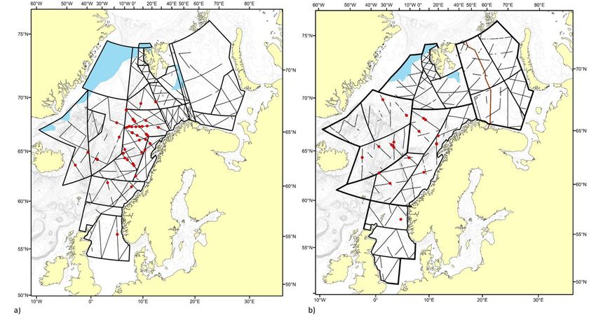
Leonard and Øien (2020)

            Figure 1. (a) White-beaked dolphin, (b) Fin whale, (c) Killer whales, and (d) Humpback whales. Photo credit: Deanna Leonard

MATERIALS AND METHODS                                                       structure that occurred in 2003 (described in the Survey Design
                                                                            section above), some blocks (FI, NOS, NC1) were surveyed
                                                                            twice, both in 2002 and 2006. Based on advice from the
Survey Design
                                                                            NAMMCO Abundance Estimates Working Group in October
The study area covers the Northeast Atlantic from the North Sea             2018 (NAMMCO, 2018), the duplicate effort in some blocks was
to the ice edge, and from the Greenland Sea in the west to the              retained and used to improve abundance estimation. The block
Barents Sea in the east. It consists of the 5 Small Management              BA2 was modified from the original BAW block mid survey cycle,
Areas (SMA) of the North Atlantic Minke Whale Implementation                in 2003. As a result, it was partially surveyed twice, and due to
(IWC, 2004): CM, ES, EB, EW, and EN (Figure 2). Within each                 differing amounts of ice cover affecting the total area of the
SMA, a block structure was fitted to create areas of similar                block, 2 separate estimates were obtained (BA2_a and BA2_b).
densities of minke whales, with survey effort distributed
                                                                            During 2008–2013, one or two vessels conducted the surveys
proportional to area. Within each block, transects were
                                                                            each year, with a total of 7 vessels operating over the 6-year
constructed as zig-zag tracks with a random starting point
                                                                            period. In 2008 the Svalbard area was surveyed; in 2009 the
(Buckland et al., 2001). Block areas used to estimate species
                                                                            North Sea; in 2010 the Jan Mayen area; in 2011 the Norwegian
density were adjusted for ice-cover. In 2003, the SMA structure
                                                                            Sea; and in 2013 the Barents Sea was surveyed.
was modified by the IWC Scientific Committee, shifting the
eastern boundary of the Barents Sea SMA westward to 28°E and                Field methodology
extending the upper boundary of North Sea SMA southward to
62°N (IWC, 2004). This necessitated splitting the blocks BAW                Both surveys used a double-platform design with two platforms
and FI each into 2 blocks, and because block FI was surveyed                that were visually and acoustically separated from each other
before the boundary change, it was further subdivided into Fl1              and thus independent. Platform 1 was positioned in a barrel on
and Fl2, and re-stratified (Figure 2a).                                     the mast above platform 2, which was located on the roof of the
                                                                            bridge. The two platforms varied in eye height depending on the
Due to the fragmentation of the strata through redefinitions of             vessel, with an average of 13.8 m for platform 1 and 9.7 m for
SMA boundaries that occurred in 2003 (IWC, 2004), it was                    platform 2.
necessary to redesign the block structure within the SMAs prior
to the 2008–2013 survey (Skaug et al., 2004). The updated block             Each platform operated continuously during daylight hours
design and names used in the 2008–2013 survey are illustrated               (between 05:00 and 23:00, depending on the latitude) with a
in Figure 2b.                                                               team of 2 observers. Each team worked on 1- or 2-hour shifts
                                                                            with teams rotating between platforms. The searching speed
The surveys                                                                 was 10 knots with surveys conducted in passing mode.
                                                                            Searching was conducted by naked eye. The designated search
In 2002–2007, two vessels operated simultaneously each
                                                                            area was the 90o sector centred around the transect line, within
summer, covering different parts of the survey area. Every year,
                                                                            1500 m of the vessel. When searching, one observer in each
the surveys began in late June and lasted until early August. In
                                                                            team scanned the port 45o sector from the transect line while
2002, the survey covered the area north of the coast of
                                                                            the other scanned the starboard 45o sector. All sightings were
Finnmark and a northeast section of the Norwegian Sea (SMA
                                                                            recorded regardless of whether they were sighted within the
EB); in 2003, the Svalbard area (SMA ES); in 2004 the North Sea
                                                                            designated search area.
area (SMA EN); in 2005, the Jan Mayen area (SMA CM); in 2006,
the entire Norwegian Sea (new SMA EW); and in 2007, the                     Observers recorded observations using a microphone
eastern Barents Sea (SMA EB). Due to the changes to the SMA                 connected to a central computer equipped with a GPS. Each

NAMMCO Scientific Publications, Volume 11                                                                                                       2
Leonard and Øien (2020)
observation documented the species, the angle from the Measures of covariates including glare, visibility, Beaufort Sea
transect line read from an angle board, the radial distance State (BSS) and weather conditions were recorded hourly
estimated by eye, and the group size. Tracking procedures were and/or when conditions changed notably. Covariate
followed for minke whales, where the observer dedicated their classifications and definitions are detailed in Øien (1995).
effort to recording each repeat surfacing until it passed abeam Acceptable survey conditions were defined as BSS of 4 or less
of the ship. During tracking procedures, the other team member and meteorological visibility greater than 1 km.
took over searching the entire 90o search area. When both
Data treatment
observers were occupied tracking minke whales, other minke
whale sightings, along with all non-target species, were Sightings used in the abundance-estimate analyses were
recorded as initial sightings only. After each completed included based on the following criteria: the sighting was
recording of a minke whale or other large whale sighting, initially detected before abeam; the sighting was recorded from
observers reported the sighting to the team leader by radio. The platform 1 or 2; and the species (or genus in the case of
platforms operated on separate radio channels to maintain Lagenorhynchus spp.) was confirmed.
independence. During the surveys, regular training in distance
estimation was conducted, including accuracy of angle-board Observations from the two independent platforms were
readings and distance estimation using buoys as targets. combined through a process of determining duplicate sightings.
When possible, duplicates were identified in the field by the
team leader operating from the bridge; otherwise, they were
determined post-cruise.
The criteria used to determine duplicates, both in the field and
in the post-cruise analysis, involved accounting for the timing
and position of the sightings relative to the vessel (given a speed
of 300 m per minute and allowing for some error in radial-
distance estimates by different observers). Since only the initial
sightings were recorded for non-target species, there was
occasionally the need to match duplicates of disparate
surfacings of the same whale. Given the relatively short
designated search distance for the target species (1500 m), it
was possible to have one platform make an initial sighting of a
whale thousands of meters away, while the second platform
observed it much later, once the ship moved closer to it. The
team leader played an important role in identifying these
duplicates in the field. When only one platform reported a
sighting, the team leader could assist by tracking the whale so
that if the other platform detected it closer to the ship, it could
be identified as a duplicate.
In rare cases where one observer of a clear pair of duplicate
sightings recorded the species as ‘unidentified large whale’
while the other confirmed the species, the positive ID was
accepted for that sighting. In cases where there was uncertainty
in species identification by one or both observers, the team
leader, operating from the bridge, used binoculars to confirm
uncertain identifications. Species identification was not always
possible, so some sightings were left recorded as ‘unidentified
large whales.’
For all duplicate sightings, the information recorded by the
platform from which the whale was first sighted was used in the
combined-platform analyses, as the analytical method used
requires that these fields be identical (Laake & Borchers, 2004).
Abundance estimates were calculated for the double platform
for all species apart from Lagenorhynchus spp. in the 2002–
2007 survey, where only a single platform (platform 1) was used
due to uncertainty in judging duplicates. The certainty in judging
duplicates improved between the 2002–2007 and 2008–2013
surveys due to a change in emphasis for the observers who
were instructed to make a greater effort to discern and report
smaller groups of dolphins rather than larger aggregations. In
earlier surveys, some observers would classify nearby groups of
dolphins as a single group, while others would classify them as
separate groups. This caused greater uncertainty in judging
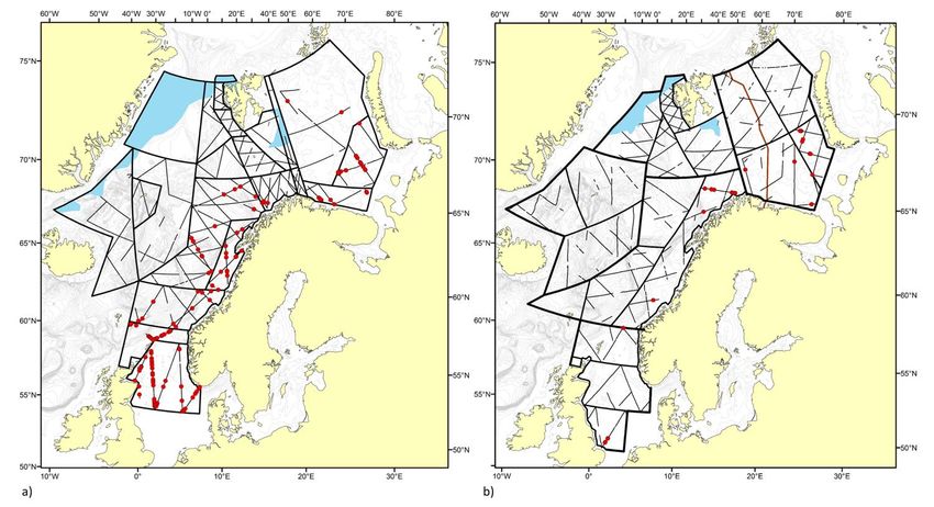
Figure 2. Survey blocks and realized search effort (Beaufort Sea State
4) on predetermined transect lines during (a) the 2002–2007 surveys and
duplicates, such that we did not feel they were reliable.
(b) the 2008–2013 surveys. The blue areas represent ice coverage.
NAMMCO Scientific Publications, Volume 11 3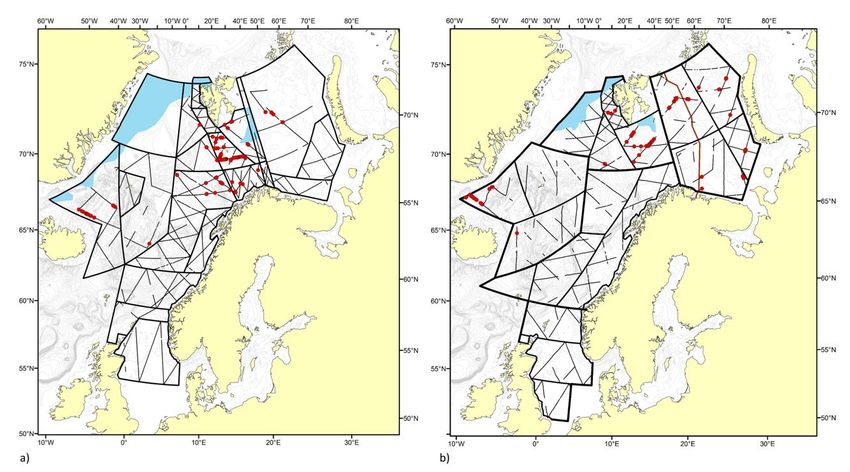
Leonard and Øien (2020)

Analysis                                                                       identity, weather, group size, glare, and visibility. Some
                                                                               covariates were aggregated into categories for simplification
These analyses were performed using the DISTANCE 7.2
                                                                               and to improve model convergence, as detailed in
software package (Thomas et al., 2010). Encounter rate and
group size for each species and each survey were estimated by                  Table 1. Data exploration also included truncation of the data
block. The effective search half-width (eshw) was estimated                    by up to 5% if it improved the test statistics (Chi-square and
using pooled data over all survey blocks (globally) for each                   Kolmogorov-Smirnov) and the shape of the q-q plot.
survey period as there were insufficient data to support
                                                                               Encounter-rate variances were estimated using R2, the default
stratified estimates.
                                                                               in the mark recapture (MRDS) engine in DISTANCE 7.2, which is
To account for perception bias by estimating p(0), mark-                       a design-based empirical estimator that assigns weights to
recapture distance sampling (MRDS) techniques were used                        transect lines based on length (Fewster et al., 2009). The
(Laake & Borchers, 2004). The fully independent platform                       confidence intervals of the abundance estimates were
design allowed for the “independent observer configuration” to                 calculated assuming that estimated abundance is log-normally
be used (Laake & Borchers, 2004). Both “full independence” (FI)                distributed (Buckland et al., 2001).
and “point independence” (PI) were tested (Laake & Borchers,
2004). Models were chosen based on a comparison of the                         RESULTS
Akaike’s information criterion (AIC) values. The “point
independence” configuration requires the estimation of 2                       General
detection functions: one for the probability of detection by one
or more observers (Distance Sampling model: DS model), and a                   In 2002–2007 a total effort of 27,009 km of transects were
second conditional detection function (Mark Recapture model:                   searched over the survey period (Figure 2a), covering a total
MR model) for detection probabilities conditioned on detection                 area of 2,962,269 sq. km. The distributions of search effort by
by the other platform (Laake & Borchers, 2004). The “full                      BSS were 3% in BSS 0, 15% in BSS 1, 22% in BSS 2, 32% in BSS 3
independence” configuration requires only the conditional                      and 28% in BSS 4. The surveys conducted between 2008–2013
detection function. The conditional detection function is                      covered a total area of 3,268,243 sq. km and 24,300 km of
modelled logistically with the same covariates available for the               transects were searched (Figure 2b). The distributions of search
primary detection function, selected based on AIC values.                      effort by BSS were 0.5% in BSS 0, 16% in BSS 1, 20% in BSS 2,
                                                                               29% in BSS 3 and 33% in BSS 4.
The detection function models were selected based on AIC,
goodness of fit test statistics, and visual inspection, particularly           In both survey cycles there were parts of the survey area that
of data around the transect line. Hazard-rate and half-normal                  were not covered due to ice and unsuitable survey conditions.
models were tested. The covariates considered were BSS, vessel                 In 2002–2007, blocks VSI and SVI were not covered due to ice

           Table 1. Covariates descriptions included to improve model fit. Some covariates were aggregated into levels for simplification.

                                                                                             Aggregated covariates
            Covariate             Description             Symbol                  Levels                        Definition

                                                                                                                BI: [0-1], BII: [2], BIII: [3-
            Beaufort              5 categories               B                    BI, BII, BIII
                                                                                                                4]

                                                                                                                good: W01-W04, bad:
            Weather               12 categories              W                    good, bad
                                                                                                                W05-W12
            Vessel                5 vessels                 Ves                          -                                    -

                                                                                                                low < 50% Max
            Visibility            numerical                  V                    high, low
                                                                                                                high > 50% Max

                                                                                  glare, no
            Glare                 4 categories               G                                                  G0: no glare, G1: glare
                                                                                  glare

            Group size            numerical                  S                           -                                    -

            Distance              numerical                  D                           -                                    -

NAMMCO Scientific Publications, Volume 11                                                                                                          4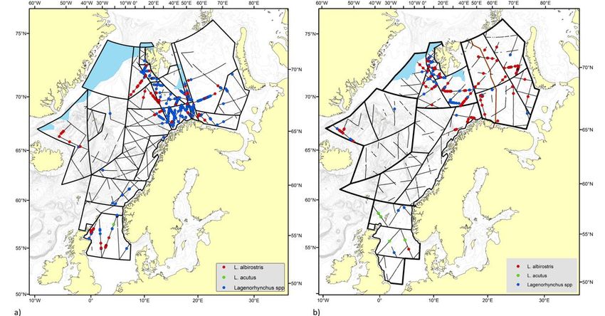
Leonard and Øien (2020)

and poor weather. In 2008–2013, block EW4 was not covered
due to consistently poor weather and parts of the northernmost
blocks (ES) were not surveyed due to ice cover. Block areas used
in calculating abundance estimates were adjusted to exclude
ice-covered areas.
Large whales
In 2002–2007 there were 893 unique records of large whale
sightings (Table 2) and of these, 218 were identified as fin
whales, 229 as sperm whales, 245 as humpback whales, 11 as
blue whales, and 1 was identified as a sei whale. 189 sightings
were categorized as ‘unidentified large whales’. In 2008–2013,
there were 611 records of large whale sightings (Table 3) and of
these, 224 were identified as fin whales, 92 as sperm whales,
179 as humpback whales, 2 as blue whales, and 1 as a sei whale.
113 were categorised as ‘unidentified large whale’.
Smaller odontocetes
There were 1042 unique records of smaller odontocete groups
sighted during the 2002–2007 survey period (Table 2). Of these,
96 were identified as killer whales, 294 as harbour porpoises,
628 as Lagenorhynchus spp., and 12 as northern bottlenose
whales. In 2008–2013, there were 487 records of small
odontocete groups sighted (Table 3) and of these, 35 were
identified as killer whales, 50 as harbour porpoises, 392 as
Lagenorhynchus spp., and 10 of the sightings were identified as
northern bottlenose whales.
The observations by platform, duplicates, and estimated p(0)
for each species are shown in Table 4. In all cases, the PI models
produced lower AICs than the FI models. Therefore, the PI
method was used exclusively. Covariates included in the final
model for each species, for both the Distance Sampling model
(DS model) and the Mark Recapture model (MR model), are
detailed in Table 5.
Fin whales
2002–2007
The sightings of fin whales are shown in Figure 3a. They were
found throughout the survey area but were especially abundant
west of Spitsbergen, in the Barents Sea, and in the western
survey blocks near Iceland/Jan Mayen (NVN, NVS, JMC). The
final detection function models used a half-normal key function,
truncated to a perpendicular distance of 4000 m and included
BSS as a covariate in the DS model (Figure 4a). The resulting
eshw was 1858 m. The abundance of fin whales was corrected
with p(0)=0.72 (CV=0.10) to 10,004 (CV=0.18, 95% CI: 6,937–          Figure 3. Distributions of sightings recorded as fin whales during (a) the
                                                                     2002–2007 surveys and (b) the 2008–2013 surveys. The blue areas
14,426). Detailed results by survey block are reported in Table
                                                                     represent ice coverage.
6a.
2008–2013
The highest encounter rate of fin whales occurred west of            Humpback whales
Spitsbergen (ES1, ES2) and in the western Iceland/Jan Mayen
                                                                     2002–2007
survey blocks (CM2, CM3) (Figure 3b). The best-fitting models
used a half-normal key function with truncation to 4000 m. The       Humpback whales were found almost exclusively around Bear
DS model was fit with BSS and weather as covariates and the          Island, in the northern Barents Sea, and in the western-most
MR model was fit with BSS as a covariate. Plots of the detection     survey block north and east of Iceland (NVS), as depicted in
probabilities for each model are shown in Figure 5a. The             Figure 6a. The best-fitting models used a half-normal key
resulting eshw was 1909 m. The abundance estimate of fin             function truncated at a perpendicular distance of 4000 m and
whales was corrected with p(0)=0.77 (CV=0.08) to be 10,861           resulted in an eshw of 2240 m. The fitted detection function and
(CV=0.26, 95% CI: 6,433–18,339) (Table 6b).                          conditional detection probability plots are shown in Figure 4b.

NAMMCO Scientific Publications, Volume 11                                                                                                    5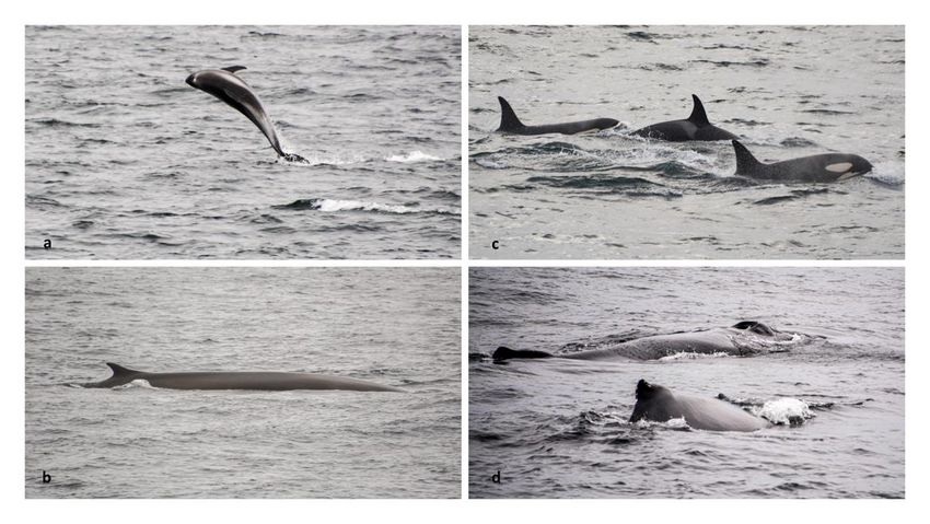
Leonard and Øien (2020)

Figure 4. 2002–2007 survey detection function curves for pooled detections (top) and the conditional detection probabilities of platform 1 (bottom)
for (a) fin whales, (b) humpback whales, and (c) sperm whales.

Figure 5. 2008–2013 survey detection function curves for pooled detections (top) and the conditional detection probabilities of platform 1 (bottom)
for (a) fin whales, (b) humpback whales, and (c) sperm whales.

Weather was included as a covariate in both the DS and the MR               Sperm whales
models. This produced a total estimate for humpback whales of
                                                                            2002–2007
9,749 (CV=0.34, 95% CI: 4,947–19,210), corrected with p(0)=
0.70 (CV=0.09) (Table 7a).                                                  Table 7a depicts the distribution of sperm whale sightings from
                                                                            the 2002–2007 sightings surveys. Most of the sightings were
2008–2013
                                                                            made in the deep waters of the Norwegian Sea, south of the
Humpback whales concentrated in 3 main areas: north and east                Mohn Ridge between Jan Mayen and Bear Island. A half-normal
of Iceland (CM2), around Bear Island (ES1), and in the northern             key function produced the best fit to the data, truncated to
Barents Sea (EB3) (Figure 6b). Detection function models were               2800 m (Figure 4c). The resulting eshw was 1564 m and the
fit with a half-normal key function truncated to 4000 m,                    probability of sighting sperm whales on the trackline was
producing an eshw of 1760 m (Figure 5b). The probability of                 estimated to be p(0)=0.81 (CV=0.06). With correction for
sighting a humpback whale on the trackline was estimated to be              perception bias, the sperm whale abundance was estimated to
p(0)=0.79 (CV=0.05). Visibility was included as a covariate in the          be 8,134 (CV=0.18, 95% CI: 5,695–11,617). Detailed estimates
DS model and weather was included in the MR model. The total                by block are detailed in Table 8a.
estimate of humpback whales (corrected for perception bias)
was 12,411 (CV=0.30, 95% CI: 6,847–22,497) (Table 7b).

NAMMCO Scientific Publications, Volume 11                                                                                                             6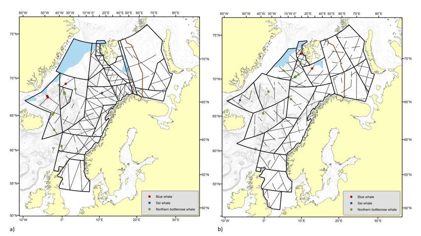
Leonard and Øien (2020)

2008–2013                                                                 Killer whales
Similar to the 2002–2007 survey, most of the sightings were               2002–2007
made over the deep waters of the Norwegian Sea (EW1), south
                                                                          Sightings of killer whales occurred mainly in the Norwegian Sea
of Jan Mayen (CM1) (Figure 7b). A half-normal key function
                                                                          south of the Mohn Ridge in block NOS (Figure 8a). They were
produced the best fit to the data truncated at 4000 m (Figure
                                                                          also abundant in the Icelandic/Jan Mayen survey blocks (NVN,
5c). The resulting eshw was 1964 m. Sperm whale abundance
                                                                          NVS). The best fitting models used a half-normal key function.
was corrected with p(0)=0.91 (CV=0.03) to a total corrected
                                                                          Data were truncated at 2000 m and resulted in an eshw of 996
estimate of 3,962 (CV=0.29, 95% CI: 2,218–7,079). Detailed
                                                                          m. BSS and weather covariates improved the fit of the DS model
results by survey block are reported in Table 8b.
                                                                          and group size improved the fit of the MR model (Figure 9a).

     Figure 6. Distributions of sightings recorded as humpback whales during (a) the 2002–2007 surveys and (b) the 2008–2013 surveys.
     The blue areas represent ice coverage.

     Figure 7. Distributions of sightings recorded as sperm whales during (a) the 2002–2007 surveys and (b) the 2008–2013 surveys. The
     blue areas represent ice coverage.

NAMMCO Scientific Publications, Volume 11                                                                                                   7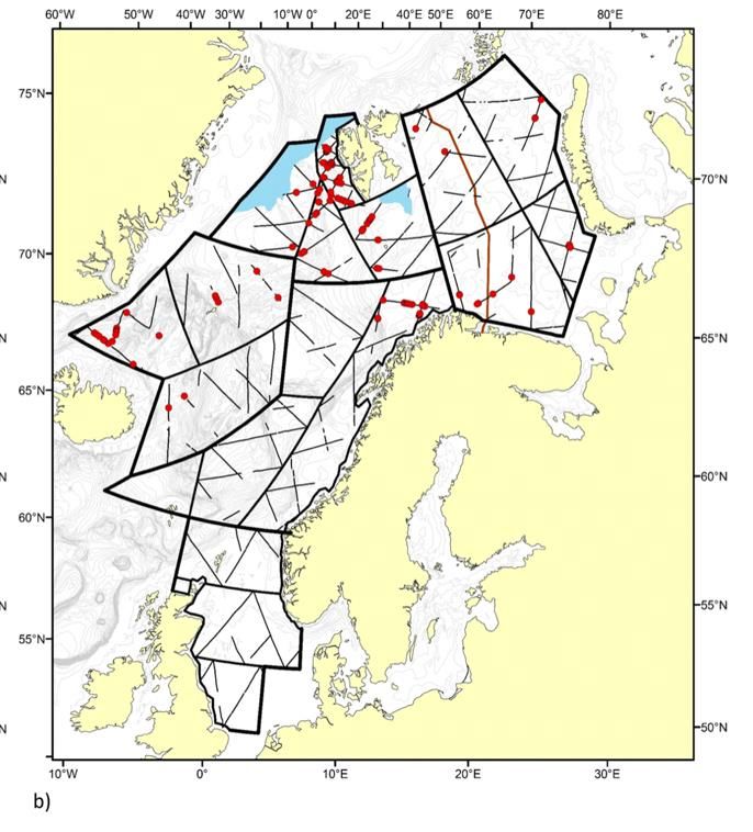
Leonard and Øien (2020)

The probability of sighting a killer whale on the trackline was             4,713–19,403). Detailed estimates by block are provided in
p(0)=0.93 (CV=0.04) and the total corrected estimate was                    Table 9b.
18,821 (CV=0.24, 95% CI: 11,525–30,735). Detailed estimates by
                                                                            Harbour Porpoises
block are reported in Table 9a.
                                                                            2002–2007
2008–2013
                                                                            Harbour porpoises were found in highest concentrations in the
As in 2002–2007, most of the sightings were made in the
                                                                            North Sea blocks NS and NC2 with additional concentrations in
Norwegian Sea (EW1, EW2) south of the Mohn Ridge. They were
                                                                            the Barents Sea (blocks KO and GA). They displayed a general
also abundant in the Icelandic/Jan Mayen survey blocks (CM1,
                                                                            shelf distribution within the study region and were absent from
CM3) (Figure 8b). Models were fit with a half-normal key
                                                                            the western and northern-most survey blocks (Figure 11a). A
function (Figure 10a). Distances were truncated at 2200 m,
                                                                            half-normal key function with distances truncated to 600 m
resulting in an eshw of 1377 m. BSS improved the fit of the MR
                                                                            generated the best fitting models, resulting in an estimated
model. Once corrected for perception bias (p(0)=0.92, CV=0.05)
                                                                            eshw=279 m and p(0)=0.52 (CV=0.15) (Figure 9b). The DS model
the total estimate for killer whales was 9,563 (CV=0.36, 95% CI:

   Figure 8. Distributions of sightings recorded as killer whales during (a) the 2002–2007 surveys and (b) the 2008–2013 surveys. The blue areas
   represent ice coverage.

   Figure 9. 2002–2007 survey detection function curves for pooled detections (top) and the conditional detection probabilities of platform 1
   (bottom) for (a) killer whales (a); harbour porpoises (b); and the detection function curve of the platform 1 detection distances for
   Lagenorhynchus spp. (c)

NAMMCO Scientific Publications, Volume 11                                                                                                          8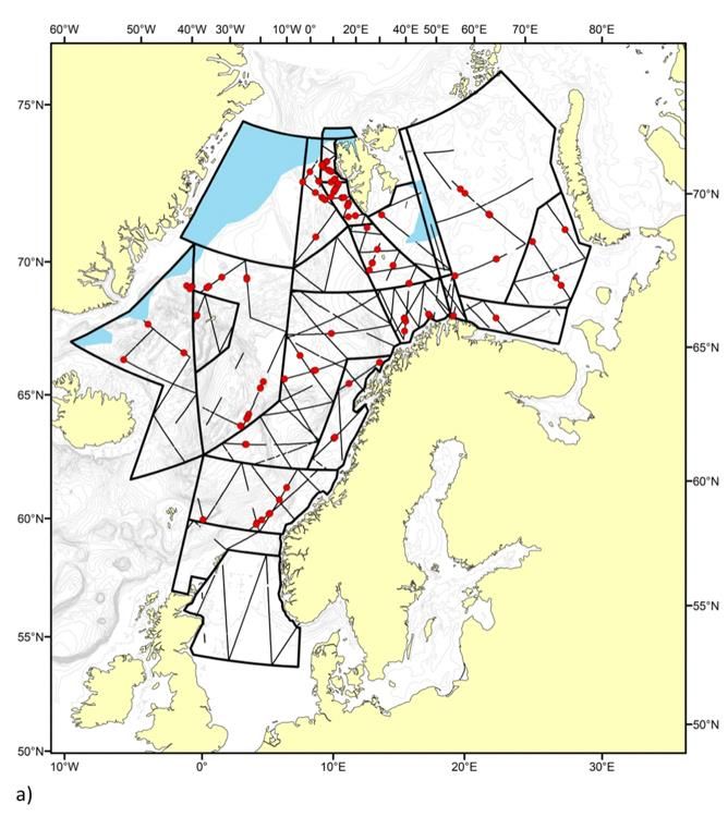
Leonard and Øien (2020)

included BSS, visibility, vessel, and group size as covariates. The          completely absent from the western and northern-most survey
MR model included the covariates BSS and weather. Once                       blocks (Figure 11b). A half-normal key function with distances
corrected for perception bias, the harbour porpoise abundance                truncated to 500 m generated the best fitting models, with an
was 189,604 (CV=0.19, 95% CI: 129,437–277,738). Detailed                     eshw of 375 m. The proportion of harbour porpoises sighted on
estimates by block are provided in Table 10a.                                the trackline was estimated to be p(0)=0.36 (CV=0.49). Both the
                                                                             DS model and MR models included BSS as a covariate (Figure
2008–2013
                                                                             10b). The corrected harbour porpoise abundance was 38,351
Harbour porpoises were sighted most commonly in the Barents                  (CV=0.58, 95% CI: 13,158–111,777). Detailed estimates by block
Sea (EB1, EB2) and the Norwegian Sea (EW1) and were                          are provided in Table 10b.

 Figure 10. 2008–2013 survey detection function curves for pooled detections (top) and the conditional detection probabilities of platform 1 (bottom)
 for killer whales (a), harbour porpoises (b), and Lagenorhynchus spp. (c).

 Figure 11. Distributions of sightings recorded as harbour porpoises during (a) the 2002–2007 surveys and (b) the 2008–2013 surveys. The blue areas
 represent ice coverage.

NAMMCO Scientific Publications, Volume 11                                                                                                           9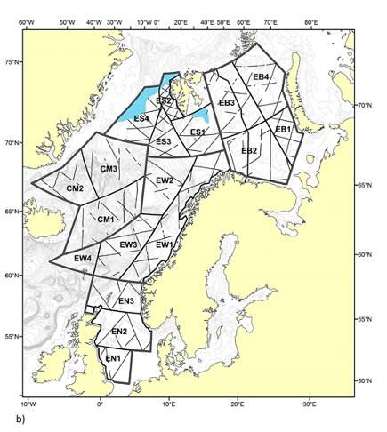
Leonard and Øien (2020)

  Table 2. Summary of effort and sightings for the 2002–2007 survey for each species by survey block and year.

                                        Total
                          Area                      Large         Fin        Humpback       Sperm         Blue     Sei      Northern     Killer    Lags     Harbor     Northern
    Year     Block                    Transect                                                                                                                                        Totals
                         sq. km                     whales       whales       whales        whales       whales   whales   bottlenose   whales    spp.**   porpoise   bottlenose
                                       length
             FI1*        78,602*       1,736          12           11             6            1                                                   115        6                        151
    2002     FI2*        16,033*        249           1                                                                                             28        1                         30
             NOS*       396,746*       4,314          28           17            12           101                              1          39        12       16           1            227
             BA1          73,918        645           11            6             5                                                                 36        1                         59
             BA2a         12,514        220           5             1            13                                                                 18                                  37
             BJ           75,479       1,228          45           13           144             1                                                   79                                 282
    2003     VSS          28,866        485           2            38                           5                                                   42                                  87
             NON          90,432        760           4                           3            23                              2          2         33                    2             69
             SV           79,929        792           16           19             2                                                                 20                                  57
             VSN          18,259        339           10           22                                                                                1                                  33
             NC1*       211586*        1,295          3             4                          1                               2          1          2        15          2             30
    2004     NC2          99,537        372                                                                                                          0        51                        51
             NS          261,311       2,154                                                                                              3         81       107                       191
             JMC          66,632        438           5             4                           3           3                  3                     0                    3             21
    2005     NVN         351,582       1,823          13           24             1            17           2                  1          13         1                    1             73
             NVS         310,021       1,834          15           14            41             1           6                  3          7         11                    3            101
             LOC          97,352       1,253          6             9                          24                                         7          1       21                         68
             FI1*        78,602*        463           7             7             1                                                                 45        4                         64
    2006
             NOS*       39,6746*       1,565          1                           3            36                   1                     23         6        2                         72
             NC1*       21,1586*        813                         6                          16                                         1          5        9                         37
             BA2b         34,850        240                                                                                                         13        1                         14
             BAE         401,721       1,783           3           11            14                                                                 39        4                         71
    2007     KO           95,965        768                         1                                                                               26       27                         54
             FI2*         16,033        129                         2                                                                                4                                   6
             GA          160,934       1,310           2            9                                                                               10       29                         50
    Total              2,962,269       27,009         189          218          245           229           11      1         12          96       628       294         12          1,935
    *partially surveyed in different years
    ** sightings from platform 1 only

NAMMCO Scientific Publications, Volume 11                                                                                                                                                      10
Leonard and Øien (2020)
Table 3. Summary of effort and sightings for the 2008–2013 survey for all species by survey block and year.
Total
Area Large Fin Humpback Sperm Blue Sei Killer Lags. Harbor Northern
Year Block transect Totals
sq. km whales whales whales whales whales whales whales spp. porpoise bottlenose
length
ES1 161,660 1,378 17 33 66 1 1 80 198
ES2 46,525 1,116 33 73 3 1 1 116 1 228
2008
ES3 118,765 1,414 6 18 4 1 26 7 62
ES4 131,447 1,348 3 4 3 1 11
EN1 95,675 765 5 5
2009 EN2 197,293 1,283 6 1 7
EN3 160,660 916 1 18 3 22
CM1 297,396 1,779 1 2 1 30 10 44
2010 CM2 177,961 958 20 25 45 1 15 106
CM3 295,929 1,002 6 9 3 2 20
EW1 333,180 2,909 5 32 31 12 24 12 116
EW2 218,943 969 2 9 5 1 17
2011
EW3 228,406 1,852 2 9 4 15
EW4* 84,625 0 0
EB1 107,105 1,199 2 9 6 3 19 39
EB2 278,964 2,122 2 7 8 10 15 10 52
2013
EB3 269,058 1,579 8 3 33 19 63
EB4 233,900 1,711 6 9 13 65 93
Total 3,268,243 24,300 113 224 179 92 2 1 35 392 50 10 1,098
* Block not surveyed due to poor weather
NAMMCO Scientific Publications, Volume 11 11Leonard and Øien (2020)
Table 4. Estimated p(0) for each species showing the total number of sightings (n), sightings by platform, and duplicates.
2002–2007 2008–2013
Species
Observations p(0) Observations p(0)
n Plat 1 Plat 2 Duplicates Estimate CV n Plat1 Plat2 Duplicates Estimate CV
Fin whales 212 137 127 52 0.724 0.100 222 159 143 80 0.772 0.083
Humpback whales 241 174 139 72 0.705 0.092 170 119 115 64 0.788 0.048
Sperm whales 229 161 150 82 0.811 0.063 94 76 64 46 0.908 0.031
Harbour porpoises 279 177 150 48 0.518 0.145 46 31 24 9 0.355 0.489
Killer whales 91 66 72 47 0.930 0.040 31 26 23 18 0.820 0.049
Lagenorhynchus spp. 597 597 - - 1.0* 0.000 354 246 261 153 0.835 0.041
*p(0) was assumed = 1 for Lagenorhynchus spp., estimated from a single platform.
Table 5. Covariates included in the final models for each species in the 2002–2007 and 2008–2013 surveys for the Distance Sampling model (DS model) and the Mark Recapture model (MR
model). Distance (D) is automatically added as a covariate in the DS Model. B=Beaufort, W=weather, Ves=vessel, V=visibility, G=glare, S=group size, D=distance.
2002–2007 2008–2013
Species DS Model MR Model DS Model MR Model
Fin whales B D B+W B
Humpback whales W W V W
Sperm whales D
Harbour porpoises B+V+Ves+S B+W B B
Killer whales B+W D+S B
Lagenorhynchus spp. - B+W+S
NAMMCO Scientific Publications, Volume 11 12Leonard and Øien (2020)
Lagenorhynchus spp. the Barents Sea (EB4) (depicted in Figure 12b). A half-normal
key function was used to fit the data (Figure 10c), with
2002–2007
covariates BSS, weather, and group size in the DS model. The
Lagenorhynchus spp. were found in almost all blocks within the eshw was 585 m, with the data truncated to 1200 m. Detection
study area, with the highest number of sightings around Bear of Lagenorhynchus spp. on the transect line was estimated to
Island (Figure 12a). A hazard-rate key function, without be p(0)=0.84 (CV=0.04). The corrected survey estimate of
covariates, provided the best fit to the data from platform 1, Lagenorhynchus spp. was 163,688 (CV=0.18, 95% CI: 112,673–
which were truncated at a perpendicular distance of 1200 m. 237,800). Block-wise estimates are detailed in Table 11b.
The detection function (Figure 9c) resulted in an eshw of 498 m
Other species
and a total Platform-1 estimate of 213,070 (CV=0.18, 95% CI:
144,720–313,690). Block-wise estimates are detailed in Table Other species recorded, for which abundance has not been
11a. As noted previously, the abundance was not corrected for estimated due to an insufficient number of observations,
perception bias. include blue whales, sei whales, and northern bottlenose
whales. Their distributions are displayed in Figure 13. No
2008–2013
sightings of pilot whales were made, but block EW4 near the
Lagenorhynchus spp. were found throughout the survey area Faroes, where they would be expected (Pike et al., 2019a,
and were most commonly sighted around Bear Island (ES1) and 2019b), has not been covered in recent surveys.
Figure 12. Distributions of sightings recorded as Lagenorhynchus spp. during (a) the 2002–2007 surveys and (b) the 2008–2013 surveys. The
blue areas represent ice coverage.
Figure 13. Distribution of blue whales, sei whales, and northern bottlenose whales sighted during (a) the 2002–2007 surveys and (b) the
2008–2013 surveys. The blue areas represent ice coverage.
NAMMCO Scientific Publications, Volume 11
13Leonard and Øien (2020)
Table 6. Estimated density and abundance of fin whales from the 2002–2007 survey (a) and the 2008–2013 survey (b). The eshw (effective
search half width (m)) was estimated for the entire study area. Encounter rate, group size, density, abundance, and upper and lower confidence
limits were estimated by block and corrected for perception bias, with the estimated p(0).
a)
Corrected 95% Confidence
Survey eshw Encounter Rate Group Size Density
Abundance Interval
Block
Estimate CV Estimate CV Estimate CV Estimate CV Lower Upper
BA1 0.016 1.030 1.67 0.000 0.006 1.036 448 1.036 12 16,228
BA2_a 0.005 0.000 1.00 0.154 0.002 0.158 84 0.158 55 128
BA2_b
BAE 0.011 0.489 1.82 0.067 0.004 0.515 1,552 0.515 517 4,662
BJ 0.011 0.352 1.08 0.076 0.004 0.371 323 0.371 142 733
FI1 0.010 0.502 1.19 0.114 0.004 0.526 287 0.526 98 842
FI2 0.013 1.279 2.50 0.000 0.005 1.284 83 1.284 4 1,863
GA 0.006 0.572 1.00 0.000 0.002 0.580 330 0.580 94 1,157
KO 0.004 0.949 3.00 0.000 0.002 0.956 146 0.956 16 1,336
SV 0.025 0.465 1.05 0.053 0.010 0.473 763 0.473 250 2,332
VSN 1,858 8.14 0.074 0.329 1.33 0.093 0.026 0.349 469 0.349 178 1,234
VSS 0.099 0.339 1.30 0.056 0.033 0.402 946 0.402 344 2,597
JMC 0.012 0.912 1.75 0.000 0.004 0.918 286 0.918 33 2,446
NVN 0.016 0.334 1.25 0.179 0.006 0.345 2,146 0.345 1 027 4,486
NVS 0.008 0.596 1.06 0.068 0.003 0.646 925 0.646 240 3,563
NON
NOS 0.004 0.448 1.31 0.156 0.001 0.486 537 0.486 207 1,394
LOC 0.007 0.620 1.13 0.044 0.003 0.630 273 0.630 57 1,306
NC1 0.005 0.465 1.11 0.112 0.002 0.461 406 0.461 147 1,119
NC2
NS
Total 0.003 0.186 10,004 0.186 6,937 14,426
b)
Corrected 95% Confidence
Survey eshw Encounter Rate Group Size Density
Abundance Interval
Block
Estimate CV Estimate CV Estimate CV Estimate CV Lower Upper
CM1 0.001 0.666 1.00 0.000 0.000 0.775 137 0.775 29 644
CM2 0.034 0.540 1.35 0.067 0.017 0.595 2,989 0.595 858 10,417
CM3 0.013 1.011 1.37 0.110 0.004 0.984 1,190 0.984 123 11,538
ES1 0.031 0.689 1.22 0.051 0.010 0.685 1,593 0.685 329 7,714
ES2 0.093 0.291 1.44 0.107 0.027 0.280 1,275 0.280 696 2,335
ES3 0.015 0.337 1.25 0.161 0.006 0.385 682 0.385 288 1,616
ES4 0.003 0.326 1.00 0.000 0.001 0.423 165 0.423 67 411
EW1 0.013 0.579 1.18 0.068 0.005 0.545 1,577 0.545 522 4,764
EW2 1,908.9 5.14
EW3
EB1 0.007 0.469 1.00 0.000 0.002 0.374 239 0.374 93 614
EB2 0.004 0.553 1.13 0.068 0.001 0.514 324 0.514 113 930
EB3 0.004 0.671 2.00 0.492 0.001 0.677 280 0.677 73 1,076
EB4 0.005 0.782 1.00 0.000 0.002 0.811 409 0.811 78 2,163
EN1
EN2
EN3
Total 0.003 0.262 10,861 0.262 6,433 18,339
NAMMCO Scientific Publications, Volume 11 14Leonard and Øien (2020)
Table 7. Estimated density and abundance of humpback whales from the 2002–2007 survey (a) and the 2008–2013 survey (b). The eshw (effective
search half width (m)) was estimated for the entire study region. Encounter rate, group size, density, abundance, and upper and lower confidence
limits were estimated by block and corrected for perception bias, with the estimated p(0).
a)
Corrected 95% Confidence
Survey eshw Encounter Rate Group Size Density
Abundance Interval
Block
Estimate CV Estimate CV Estimate CV Estimate CV Lower Upper
BA1 0.008 0.457 1.00 0.000 0.003 0.478 210 0.478 38 1,163
BA2_a 0.073 0.000 1.23 0.107 0.026 0.004 331 0.170 215 509
BA2_b
BAE 0.010 0.603 1.28 0.096 0.004 0.618 1,501 0.618 412 5,470
BJ 0.152 0.510 1.32 0.055 0.054 0.520 4,040 0.520 1,304 12,515
FI1 0.005 0.295 1.42 0.119 0.002 0.314 124 0.314 64 238
FI2
GA
KO
SV 0.003 0.701 1.00 0.000 0.001 0.713 72 0.713 14 364
VSN 2,240 6.36
VSS
JMC
NVN 0.001 1.036 1.00 0.000 0.000 1.048 72 1.048 10 501
NVS 0.027 0.734 1.27 0.016 0.009 0.742 2,925 0.742 644 13,292
NON 0.004 0.959 1.00 0.000 0.001 0.970 114 0.970 4 3,273
NOS 0.003 0.435 1.00 0.000 0.001 0.453 359 0.453 147 879
LOC
NC1
NC2
NS
Total 0.004 0.311 9,749 0.336 4,947 19,210
b)
Corrected 95% Confidence
Survey eshw Encounter Rate Group Size Density
Abundance Interval
Block
Estimate CV Estimate CV Estimate CV Estimate CV Lower Upper
CM1 0.001 0.915 1.00 0.000 0.000 0.924 61 0.919 10 371
CM2 0.051 0.609 1.14 0.066 0.022 0.578 3,747 0.574 1,073 13,084
CM3
ES1 0.067 0.460 1.59 0.022 0.026 0.509 3,963 0.499 1,197 13,117
ES2 0.003 0.646 1.00 0.000 0.001 0.659 46 0.652 12 175
ES3 0.002 0.910 1.00 0.000 0.001 0.919 93 0.914 14 618
ES4
EW1 0.002 0.668 1.25 0.148 0.001 0.681 210 0.674 55 804
EW2 1,760.3 5.11
EW3
EB1 0.005 0.916 1.00 0.000 0.002 0.925 197 0.920 23 1,704
EB2 0.006 0.692 1.63 0.167 0.002 0.704 628 0.697 158 2,495
EB3 0.028 0.710 1.42 0.136 0.011 0.721 2,754 0.715 673 11,272
EB4 0.008 0.459 1.06 0.045 0.003 0.473 713 0.466 253 2 013
EN1
EN2
EN3
Total 0.004 0.305 12,411 0.295 6,847 22,497
NAMMCO Scientific Publications, Volume 11 15Leonard and Øien (2020)
Table 8. Estimated density and abundance of sperm whales from the 2002–2007 survey (a) and the 2008–2013 survey (b). The eshw (effective
search half width (m)) was estimated for the entire study region. Encounter rate, group size, density, abundance, and upper and lower
confidence limits were estimated by block and corrected for perception bias, with the estimated p(0).
a)
Corrected 95% Confidence
Survey eshw Encounter Rate Group Size Density
Abundance Interval
Block
Estimate CV Estimate CV Estimate CV Estimate CV Lower Upper
BA1
BA2_a
BA2_b
BAE
BJ 0.001 0.953 1.00 0.000 0.000 0.957 24 0.957 4 162
FI1 0.000 0.977 1.00 0.000 0.000 0.980 14 0.980 2 86
FI2
GA
KO
SV
VSN 1,564 5.33
VSS 0.008 0.969 1.00 0.000 0.004 0.972 118 0.972 12 1,117
JMC 0.003 0.912 1.00 0.000 0.00 0.566 137 0.566 32 578
NVN 0.007 0.407 1.12 0.091 0.004 0.440 1,448 0.440 565 3,711
NVS 0.001 1.019 2.00 0.000 0.000 1.022 134 1.022 19 935
NON 0.024 0.259 1.04 0.034 0.012 0.259 1,129 0.259 452 2,822
NOS 0.016 0.223 1.01 0.008 0.009 0.228 3,680 0.228 2,317 5,845
LOC 0.010 0.575 1.00 0.000 0.008 0.643 737 0.643 147 3,697
NC1 0.007 0.798 1.06 0.009 0.003 0.839 714 0.839 128 3,986
NC2
NS
Total 0.003 0.180 8,134 0.180 5,695 11,617
b)
Corrected 95% Confidence
Survey eshw Encounter Rate Group Size Density
Abundance Interval
Block
Estimate CV Estimate CV Estimate CV Estimate CV Lower Upper
CM1 0.017 0.531 1.06 0.031 0.005 0.563 1,516 0.563 457 5,032
CM2
CM3
EN3
ES1 0.001 1.179 1.00 0.000 0.000 1.189 35 1.189 3 380
ES2 0.001 0.969 1.00 0.000 0.000 0.973 11 0.973 2 72
ES3 0.001 1.001 1.00 0.000 0.000 1.006 23 1.006 3 177
ES4
EW1 0.011 0.417 1.06 0.031 0.003 0.447 1,080 0.447 428 2,726
1,964.1 8.42
EW2 0.009 0.320 1.00 0.000 0.003 0.333 559 0.333 239 1,307
EW3 0.005 0.318 1.00 0.000 0.001 0.331 305 0.331 145 640
EB1
EB2 0.005 0.966 1.09 0.000 0.002 0.970 434 0.970 72 2,593
EB3
EB4
EN1
EN2
EN3
Total 0.001 0.286 3,962 0.286 2,218 7,079
NAMMCO Scientific Publications, Volume 11 16Leonard and Øien (2020)
Table 9. Estimated density and abundance of killer whales from the 2002–2007 survey (a) and the 2008–2013 survey (b). The eshw (effective search
half width (m)) was estimated for the entire study region. Encounter rate, group size, density, abundance, and upper and lower confidence limits
were estimated by block and corrected for perception bias, with the estimated p(0).
a)
Corrected 95% Confidence
Survey eshw Encounter Rate Group Size Density
Abundance Interval
Block
Estimate CV Estimate CV Estimate CV Estimate CV Estimate CV Lower Upper
BA1
KO
LOC 0.024 0.337 4.17 0.041 0.015 0.353 1,469 0.353 605 3,568
NC1 0.008 0.840 6.30 0.798 0.003 0.814 717 0.814 135 3,815
NC2
NON 0.004 0.499 1.00 0.000 0.002 0.458 205 0.458 41 1,015
NOS 0.043 0.213 4.45 0.101 0.023 0.243 9,134 0.243 5,612 14,866
NS 0.006 0.918 3.97 0.049 0.003 0.927 696 0.927 94 5,157
NVN 0.019 0.579 2.45 0.097 0.015 0.695 5,180 0.695 1,291 20,788
NVS 0.009 0.837 2.68 0.052 0.003 0.758 1,016 0.758 222 4,654
SV 995.91 7.5
BA2_a
VSN
VSS
BA2_b
BAE 0.002 0.992 4.00 0.000 0.001 1.000 404 1.000 60 2,726
BJ
FI1
FI2
GA
JMC
Total 0.006 0.242 18,821 0.242 11,525 30,735
b)
Corrected 95% Confidence
Survey eshw Encounter Rate Group Size Density
Abundance Interval
Block
Estimate CV Estimate CV Estimate CV Estimate CV Estimate CV Lower Upper
CM1 0.028 0.220 5.21 0.186 0.011 0.370 3,528 0.388 1,601 7,776
CM2
CM3 0.010 0.821 3.33 0.211 0.003 0.836 1,049 0.836 147 7,497
ES1
ES2
ES3
ES4
EW1 0.018 0.625 5.87 0.125 0.008 0.771 3,048 0.783 708 13,112
EW2 1,377.3 14.43 0.013 0.444 2.63 0.061 0.005 0.432 1,194 0.416 462 3,084
EW3 0.009 0.510 4.25 0.284 0.003 0.535 744 0.535 237 2,343
EB1
EB2
EB3
EB4
EN1
EN2
EN3
Total 0.003 0.355 9,563 0.362 4,713 19,403
NAMMCO Scientific Publications, Volume 11 17Leonard and Øien (2020)
Table 10. Estimated density and abundance of harbour porpoises from the 2002–2007 survey (a) and the 2008–2013 survey (b). The eshw
(effective search half width (m)) was estimated for the entire study region. Encounter rate, group size, density, abundance, and upper and lower
confidence limits were estimated by block and corrected for perception bias, with the estimated p(0).
a)
Corrected 95% Confidence
Survey eshw Encounter Rate Group Size Density
Abundance Interval
Block
Estimate CV Estimate CV Estimate CV Estimate CV Lower Upper
BA1 0.002 1.058 1.00 0.000 0.004 1.081 274.68 1.081 8.25 9,144
BA2_a
BA2_b 0.004 0.000 1 0.040 0.026 0.206 1,239 0.206 829 1,851
BAE 0.003 0.478 1.43 0.299 0.015 0.516 5,972 0.516 2,083 17,119
BJ
FI1 0.007 0.436 1.41 0.107 0.018 0.494 1,413 0.494 520 3,837
FI2 0.003 0.468 1.00 0.000 0.012 0.512 191 0.512 52 703
GA 0.032 0.463 1.25 0.124 0.128 0.387 20,545 0.387 9,065 46,561
KO 0.079 0.731 1.61 0.153 0.255 0.595 24,504 0.595 5,844 102,737
SV
VSN 279.2 4.71
VSS
JMC
NVN
NVS
NON
NOS 0.003 0.431 1.09 0.069 0.013 0.472 5,266 0.472 2,108 13,154
LOC 0.024 0.279 1.30 0.076 0.080 0.304 7,768 0.304 4,006 15,063
NC1 0.015 0.273 1.26 0.066 0.064 0.313 13,548 0.313 6,994 26,244
NC2 0.180 0.118 1.23 0.066 0.669 0.191 66,551 0.191 45,432 97,486
NS 0.065 0.387 1.36 0.086 0.162 0.374 42,332 0.374 18,283 98,014
Total 0.063 0.194 189,604 0.194 129,437 277,738
b)
Corrected 95% Confidence
Survey eshw Encounter Rate Group Size Density
Abundance Interval
Block
Estimate CV Estimate CV Estimate CV Estimate CV Lower Upper
CM1
CM2
CM3
ES1 0.001 0.995 1.00 0.000 0.008 1.158 1,231 1.158 153 9,904
ES2
ES3
ES4
EW1 0.004 0.700 1.00 0.000 0.031 1.063 10,304 1.063 1,679 63,228
EW2 375.2 10.79
EW3
EB1 0.019 0.426 1.30 0.079 0.132 0.690 14,107 0.690 3,790 52,514
EB2 0.007 0.552 1.29 0.250 0.028 0.544 7,683 0.544 2,712 21,761
EB3
EB4
EN1 0.007 0.765 1.5 0.000 0.011 0.869 1,050 0.869 152 7,240
EN2
EN3 0.003 0.656 1 0.000 0.025 0.853 3,976 0.853 733 21,572
Total 0.011 0.575 38,351 0.575 13,158 111,777
NAMMCO Scientific Publications, Volume 11 18Leonard and Øien (2020)
Table 11. Estimated density and abundance of Lagenorhynchus spp. for platform 1 from the 2002–2007 survey (a) and for the combined-platform
data for the 2008–2013 survey (b). The eshw (effective search half width (m)) was estimated for the entire study area. Encounter rate, group size,
density, abundance, and upper and lower confidence limits were estimated by block.
a)
Platform 1 95% Confidence
Survey eshw Encounter Rate Group Size Density
Abundance Interval
Block
Estimate CV Estimate CV Estimate CV Estimate CV Lower Upper
BA1 0.029 1.058 3.21 0.321 0.054 1.091 4,028 1.086 127 127,860
BA2_a 0.082 0.000 2.94 0.171 0.166 0.179 2,079 0.170 1,465 2,951
BA2_b 0.054 0.000 5.15 0.209 0.277 0.216 9,663 0.242 5,761 16,208
BAE 0.024 0.733 4.88 0.075 0.082 0.740 32,966 0.740 7,257 149,760
BJ 0.056 0.449 4.65 0.109 0.195 0.449 14,685 0.466 5,300 40,688
FI1 0.075 0.199 5.79 0.074 0.373 0.219 29,279 0.219 18,484 46,381
FI2 0.079 0.289 5.87 0.184 0.373 0.332 6,172 0.332 2,711 14,053
GA 0.008 0.630 6.27 0.266 0.048 0.737 7,767 0.725 1,870 32,260
KO 0.033 0.574 4.68 0.114 0.144 0.604 13,858 0.589 3,222 59,601
SV 0.027 0.307 3.95 0.164 0.088 0.358 7,048 0.368 3,184 15,604
VSN 494.8 0.062 0.003 0.918 3.00 0.000 0.009 0.919 163 0.919 14 1,947
VSS 0.093 0.313 3.38 0.139 0.278 0.349 8,035 0.343 3,525 18,313
JMC
NVN 0.001 0.941 1.00 0.000 0.001 0.942 163 0.942 32 1,181
NVS 0.005 0.494 1.00 0.212 0.022 0.543 8,035 0.550 2,204 20,879
NON 0.018 0.743 4.00 0.191 0.075 0.760 6,810 0.760 477 97,220
NOS 0.002 0.574 5.43 0.186 0.013 0.602 5,087 0.602 1,607 16,100
LOC 0.001 1.001 6.00 0.000 0.005 1.002 471 1.002 47 4,743
NC1 0.003 0.584 6.83 0.684 0.013 1.460 2,849 1.049 376 21,573
NC2
NS 0.044 0.447 5.20 0.098 0.197 0.232 51,445 0.460 17,252 153,410
Total 213,070 0.184 144,720 313,690
b)
Corrected 95% Confidence
Survey eshw Encounter Rate Group Size Density
Abundance Interval
Block
Estimate CV Estimate CV Estimate CV Estimate CV Lower Upper
CM1
CM2 0.039 0.570 3.21 0.142 0.039 0.022 6,876 0.560 2,010 23,520
CM3 0.011 0.954 3.56 0.112 0.011 0.010 3,162 0.959 342 29,267
ES1 0.181 0.324 3.26 0.093 0.213 0.064 34,389 0.301 16,569 71,376
ES2 0.285 0.108 2.67 0.087 0.279 0.038 12,969 0.135 9,725 17,295
ES3 0.055 0.417 3.52 0.081 0.058 0.024 6,933 0.410 2,720 17,676
ES4 0.002 1.037 1.40 0.034 0.002 0.002 285 1.043 35 2,296
EW1 0.035 0.460 4.50 0.088 0.030 0.014 10,066 0.461 3,851 26,314
EW2 585.19 3.86
EW3
EB1 0.008 0.599 5.04 0.157 0.009 0.005 936 0.621 199 4,396
EB2 0.042 0.447 5.43 0.160 0.035 0.015 9,775 0.433 3,970 24,069
EB3 0.053 0.268 4.29 0.138 0.049 0.012 13,097 0.242 7,816 21,944
EB4 0.205 0.466 5.68 0.119 0.177 0.087 41,426 0.489 14,026 122,352
EN1
EN2 0.025 0.241 6.14 0.362 0.023 0.007 4,632 0.290 2,356 9,108
EN3 0.131 0.688 6.09 0.062 0.119 0.082 19,141 0.685 2,740 133,699
Total 0.049 0.009 163,688 0.182 112,673 237,800
NAMMCO Scientific Publications, Volume 11 19Leonard and Øien (2020)
DISCUSSION AND CONCLUSIONS Availability bias
The corrected estimates account for perception bias by
Bias and estimation issues estimating for the values of p(0), but do not correct for
Survey coverage availability, which may be a concern for sperm whales in this
study. Given that sperm whales have long dive times (Drouot,
Ice coverage hampered effort in the northernmost regions of Gannier, & Goold, 2004; Watkins, Moore, Tyack, 1985), they
the study area. In 2002–2007, the entire SVI block was not may remain submerged during vessel passage, and therefore
surveyed due to ice. However, given that SVI accounted for only undetectable. Availability bias is likely less of a concern for fin
2% of the total sightings (all species) in the previous survey and humpback whales, which exhibit shorter dives (Dolphin,
period (Øien, 2009), the lack of effort in this area is not expected 1987; Panigada, Zanardelli, Canese, & Jahoda, 1999) and are
to have had a large effect on total abundance. In 2008–2013, ice therefore more likely to be detected within the window of time
also reduced the survey area coverage in the northern regions that they are in proximity to the ship. This should also not be a
by 2.4%. Additionally, the EW4 block was not surveyed in 2008– concern with small odontocete species because they tend to
2013 due to poor weather. However, the EW4 block was also surface frequently and display conspicuous surface behaviour.
not covered in the 2002–2007 survey, nor in the earlier 1996–
2001 and 1995 surveys because it was not included as part of Duplicate judgement
the SMAs under the minke whale RMP until 2003 (Øien, 2009;
Our methods for recording observations of non-target
IWC, 2004).
species—by recording only initial observations, without
Species identification tracking—likely results in a higher level of uncertainty in judging
duplicates compared to survey designs with tracking, such as
This study used survey methods specifically designed for minke the Buckland-Turnock (BT) method (Buckland & Turnock, 1992).
whales (Skaug et al., 2004), which resulted in less optimal data The level of uncertainty is also likely higher in our surveys
collection for other species. The effective search half-width because the analyses rely heavily on post-cruise duplicate
(eshw) for minke whales is in the range of half to one third of judgements and a largely subjective approach. Developing a
that for larger baleen whales. The designated search area for more empirical and reproducible method, like that used for
the observers was within 1500 m of the ship and observers were minke whales (Bøthun et al., 2009; Solvang et al., 2015), would
instructed to dedicate more of their effort to look for minke reduce the potential error associated with judging duplicates.
whales and also track them; thus, the detection of large whales Additionally, including a confidence rating would allow for a
was likely reduced by these patterns. sensitivity analysis of the effect of error in duplicate judgement.
Some negative bias was likely introduced in the abundance Responsive movement
estimates given that the surveys were conducted in passing
mode and none of the sightings were closed upon. An Responsive movement (i.e. when animals move toward or away
examination of effective search half-widths for ‘unidentified from the ship before they are first detected), is a source of
large whale’ sightings, truncated at 4000m, resulted in potential bias in any line transect survey studying cetaceans
estimates of 2107 m (CV=0.06) in 2002–2007 and 2509 m (Buckland et al., 2001). Movement toward the ship would result
(CV=0.07) in 2008–2013, indicating that they are associated in a larger than expected number of sightings near the trackline
with greater sighting distances. It can therefore be assumed (positive bias), whereas avoidance behaviour would have the
that the unidentified sightings do not bias the estimates opposite effect. Avoidance behaviour has been detected in
proportional to their occurrence in the dataset. Additionally, an harbour porpoises (Palka & Hammond, 2001), while white-
effort to improve identifications has reduced the proportion of beaked dolphins have been shown to display both attraction
‘unidentified large whales’ in 2002–2007 and 2008–2013 to and avoidance behaviour, depending on their distance from the
19%, down from 30% in 1996–2001 (Øien, 2009). We did not observation platform (Hammond et al., 2002; Palka &
allocate unidentified whales to species based on their Hammond, 2001). Given the designated search distance for
occurrence in the dataset. The effect of uncertainty in species minke whales in the survey (1500 m), it is possible that
identification could be measured in future surveys by including responsive movement could occur with small odontocetes
a confidence rating for each identification, which would allow before they are first detected.
for a sensitivity analysis of the magnitude of bias in species
Evidence for responsive movement in baleen whales is more
identification.
mixed. A 2007 survey conducted in European waters found
Pooling robustness some evidence that fin whales were attracted to vessels
(Macleod et al., 2009), whereas a similar survey in 2016 found
The detection functions and effective search widths were fitted
no responsive movement (Hammond et al., 2017). Similarly,
over the complete survey region because most blocks did not
minke whale avoidance behaviour has been detected in some
yield enough sightings to allow separate detection functions to
surveys (Palka & Hammond, 2001), but not in others (Paxton,
be fitted. This may lead to bias in the estimates for some blocks
Gunnlaugsson, & Mikkelsen, 2009). These findings suggest that
if the detection distances vary between blocks. The bias is
responsive movement may be survey-specific and depend on
hopefully low simply due to the consideration that the survey
region, vessel type, and possibly other factors. Our survey did
blocks with the highest estimates—and therefore the greatest
not measure responsive movement; thus, there is likely some
vulnerability to bias—also had the greatest influence over the
unaccounted-for bias, although the degree and direction are
detection functions.
unknown.
NAMMCO Scientific Publications, Volume 11 20Leonard and Øien (2020)
Distance estimation Additional variance due to year-to-year shifts in distribution has
been accounted for in minke whale estimates (Bøthun et al.,
There is a large potential for bias in distance measurements in 2009; Solvang et al., 2015). The estimates from prior synoptic
line transect surveys such as ours, which rely on naked-eye and multi-year surveys and knowledge about population
estimates of distance by trained observers (Leaper, Burt, growth are used to model the random effects and estimate
Gillespie, & Macleod, 2010). Error of this type can bias additional variance assuming a closed population based on
abundance estimates by influencing the detection function genetic evidence and historic catch statistics. Corresponding
models and affecting the identification of duplicate sightings
(Buckland et al., 2001). Leaper et al. (2010) have demonstrated information is not available for the non-target species that are
that both distance and angle errors make a substantial locally abundant in smaller parts of the survey area.
contribution to the variance of abundance estimates and may
Encounter rate variance
cause considerable bias. They also found that naked eye
estimates were negatively biased, but non-linear in that Variance in estimating encounter rate can be problematic for
observers tended to overestimate shorter distances and species other than minke whales, for which this survey was
underestimate greater distances. designed. Ideally, a transect design is stratified across a species’
density in order to ensure precision in estimating the encounter
To mitigate error in distance estimation, observers received
rate variance (Buckland et al., 2001). The survey stratification
regular training using buoys as targets and newer observers
was not considered for species other than minke whales, which
were paired with more experienced observers. Observers also
may affect the precision of the estimates for other species. To
tested and trained their distance estimation skills
aim for higher precision, a spatial modelling method could be
opportunistically using floating objects (such as buoys and
applied to take spatial variation into account. This type of
birds) by estimating their distance, then verifying distances with
analysis has been shown to reveal habitat preferences of minke,
a stopwatch using the speed of the vessel (300m/min). Leaper
fin and sperm whales and Lagenorhynchus dolphins (Skern-
et al. (2010) have shown that using measurements of distance
Mauritzen, Skaug, & Øien, 2009).
to objects at the surface such as buoys, were not predictive of
the actual biases found in measurements during the surveys. In Harbour porpoise estimates and Beaufort Sea State
future surveys, more could be done to reduce this type of error
Typically for harbour porpoises, only survey effort at a BSS of 2
by incorporating a means of validating some proportion of the
or less is used to estimate abundance, due to a rapid decline in
measurements, for example using cameras or reticle binoculars.
detection at higher sea states (Barlow, 1988; Hammond et al.,
Distributional shifts 2002). This approach was tested initially; however, our surveys
exhibited a relatively high encounter rate at higher BSS
Given that the survey is conducted over a multi-year period any
compared to what has been observed in other multi-species
shifts in distribution between survey years and between survey
surveys (e.g. Hammond et al., 2002) and lower variance when
blocks could have an effect on the abundance estimates. To
using total effort. As discussed at the NAMMCO Abundance
reduce additional variance due to distributional shifts, the goal
Estimates Working Group meeting in October 2019, due to
of the surveys is to cover each minke whale SMA within one
these factors it was agreed that total effort (BSS 4 or less) could
survey year (Skaug et al., 2004). This was achieved in the 2008–
be used for all of our survey cycles (NAMMCO, 2019). Given that
2013 survey cycle. However, in the 2002–2007 cycle, some
the maximum sighting distance for harbour porpoises in these
SMAs were surveyed over multiple years and within the SMAs,
surveys was 600 m, and observers were asked to focus within a
some blocks were surveyed twice (NOS, FI), increasing the
1500 m range to detect minke whales, our survey method might
potential for this type of variance. As a result, there may be
generate reasonable abundance estimates for harbour
additional variance in the minke whale estimates for the 2002–
porpoises.
2007 survey due to the added potential for the
duplication/omission of sightings between years. The block Comparison to past surveys
design is for minke whales; thus, constraining the area surveyed
to a single SMA in a given year doesn’t necessarily reduce Fin whales
additional variance for other species, although it may help for The fin whale estimates for both surveys were very similar with
more regional species (such as small odontocetes) due to the a total abundance estimate of 10,004 (CV=0.19, 95% CI: 6,937–
fact that the minke whale SMAs are oceanographic regions with 14,426) in 2002–2007 and 10,861 (CV=0.26, 95% CI: 6,433–
natural physical and biological distinctions. 18,339) in 2008–2013. Taking our corrections for perception
Variance due to distributional shifts likely differs between bias into account (0.72 CV=0.10 in 2002–2007 and 0.77 CV=0.08
species. Killer whales in the Norwegian Sea and Lagenorhynchus in 2008–2013), the previous uncorrected estimates of 10,369
spp. in the Barents Sea, for example, are local populations with CV=0.24, 95% CI: 6,277–17,128) in 1996–2001 and 5,034
large home ranges and their distribution is likely to vary within (CV=0.21, 95% CI: 3,314–7,647) in 1995 are within the range of
and between seasons in relation to prey distribution our estimates (noting that the 1995 survey did not cover block
(Christensen, 1982, 1988; Øien, 1996). Other species like NVS, which was an important area for fin whales in all other
humpback whales, which are mostly migratory, show a surveys) (Øien, 2009).
generally consistent pattern of annual habitat use (Kennedy et The distribution of fin whales in our surveys was consistent with
al., 2013), but they can also display complex variation in past surveys where fin whales were most abundant in the
distribution affected by larger climatological patterns as well as Icelandic blocks (JMC, NVN, NVS; CM1, CM2, CM3) and in the
small-scale local effects (Keen et al., 2017; Visser, Hartman, Svalbard blocks along the continental slope from Bear Island
Pierce, Valavanis, & Huisman, 2011). ranging northwards to the top of Spitsbergen (VSS, VSN; ES1,
ES2) (Øien, 2009).
NAMMCO Scientific Publications, Volume 11 21You can also read