Evaluating the Safety and Performance of Electric Micro-Mobility Vehicles
←
→
Page content transcription
If your browser does not render page correctly, please read the page content below
Evaluating the Safety and Performance
of Electric Micro-Mobility Vehicles
Comparing E-bike, E-scooter and Segway based on Objective
and Subjective Data from a Field Experiment
Master’s thesis in Systems, Control and Mechatronics

LUCAS BILLSTEIN
CHRISTOFFER SVERNLÖV

DEPARTMENT OF MECHANICS AND MARITIME SCIENCES
C HALMERS U NIVERSITY     OF   T ECHNOLOGY
Gothenburg, Sweden 2021
www.chalmers.se
Master’s thesis 2021:36

Evaluating the Safety and Performance of Electric
             Micro-Mobility Vehicles

 Comparing E-bike, E-scooter and Segway based on Objective and
           Subjective Data from a Field Experiment

                    LUCAS BILLSTEIN
                 CHRISTOFFER SVERNLÖV

            Department of Mechanics and Maritime Sciences
                      Division of Vehicle Safety
                Unit of Crash Analysis and Prevention
              Chalmers University of Technology
                      Gothenburg, Sweden 2021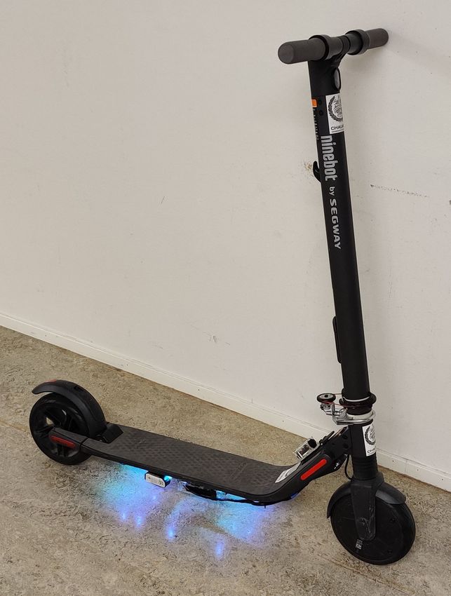
Evaluating the Safety and Performance of Electric Micro-Mobility Vehicles
Comparing E-bike, E-scooter and Segway based on Objective and Subjective Data
from a Field Experiment
LUCAS BILLSTEIN
CHRISTOFFER SVERNLÖV

© LUCAS BILLSTEIN, 2021.
© CHRISTOFFER SVERNLÖV, 2021.

Supervisor: Alexander Rasch, Department of Mechanics and Maritime Sciences
Supervisor: Christian-Nils Åkerberg Boda, Autoliv
Examiner: Marco Dozza, Department of Mechanics and Maritime Sciences

Master’s Thesis 2021
Department of Mechanics and Maritime Sciences
Division of Vehicle Safety
Unit of Crash Analysis and Prevention
Chalmers University of Technology
SE-412 96 Gothenburg
Telephone +46 31 772 1000

Cover: A picture of the e-bike, e-scooter and Segway used in the study.

Typeset in LATEX, template by Magnus Gustaver
Department of Mechanics and Maritime Sciences
Gothenburg, Sweden 2021

iv
Evaluating the Safety and Performance of Electric Micro-Mobility Vehicles
Comparing E-bike, E-scooter and Segway based on Objective and Subjective Data
from a Field Experiment
LUCAS BILLSTEIN
CHRISTOFFER SVERNLÖV
Department of Mechanics and Maritime Sciences
Chalmers University of Technology

Abstract
The rapid increase in popularity of electric micro-mobility vehicles has led to an
increasing amount of injuries. A large proportion of injuries are related to the ve-
hicles themselves, therefore, a thorough investigation of their safety is needed. The
purpose of this thesis was to collect conclusive evidence for or against the safety level
of e-bikes, e-scooters and Segways in terms of stability, maneuverability and rider
comfort. A regular bike was used as well to compare with. Rider kinematics data
were recorded by sensors mounted on each of the vehicles together with a stationary
LIDAR sensor. Thirty-four voluntary participants performed four different tasks
with each of the vehicles. Afterwards, they filled in a questionnaire regarding the
experienced safety and performance of the vehicles. A set of performance indicators
were studied to be able to compare the vehicles and establish the safety of each
vehicle.

Results suggest that the e-bike and the e-scooter performed very well in terms of
rider comfort and stability. The e-scooter also had good maneuverability, but lacked
in safety due to bad braking performance. The least safe vehicle was the Segway
which was rated the least safe by the participants and performed the worst according
to the performance indicators in high speed scenarios. There were however scenarios
at low speed, with the Segway that had comparable results with the other vehicles.

Future studies could include other micro-mobility vehicles or other tasks. Exper-
iments in a more naturalistic settings could provide valuable data to extend the
results presented in this thesis. The results from this thesis could be used to help
improve the design of electric micro-mobility vehicles and contribute to guidelines
for infrastructure design and policy making.

Keywords: safety, performance, micro-mobility, e-scooter, e-bike, Segway

                                                                                       v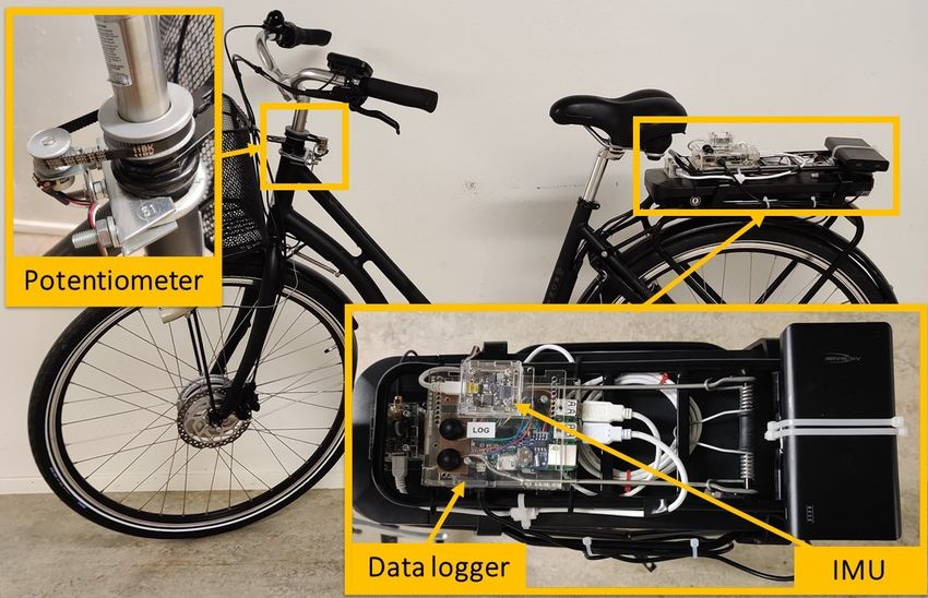
Acknowledgements
Thank you to our supervisor Alexander Rasch for supporting our work with thought-
ful insights and recommendations, and for always gladly answering to questions.
Your support and positive comments helped us get through stressful periods of this
thesis.

Thank you to our supervisor from Autoliv, Christian-Nils Åkerberg Boda for all the
help and discussion about technical details such as the orientation estimate. Your
humor and positive attitude was always welcome. Thank you Christian-Nils for al-
ways thinking one step further and challenging us throughout the whole thesis.

Thank you to Marco Dozza, our examiner, for showing up on our meetings with
great insights and ideas. Thank you so much for making this master’s thesis possi-
ble.

Thank you to all three, Alexander, Christian-Nils and Marco for being very easy to
work with.

Thank you to Alessio Violin for giving an introduction to the instrumentation.

Thank you to our opponents, Felicia Österberg and Paula Ek, for their great dis-
cussion after our presentation and their detailed feedback on our report.

Thank you to SAFER for advertising our poster that was made to gather partici-
pants.

Thank you to all the participants that participated in the field experiment. Without
all 34 of you, this thesis would not have turned out the way it did.

Thank you to the kind employees at Autoliv which listened to our "mid-term" pre-
sentation and gave great feedback.

We would also like to thank Trafikverket for sponsoring this thesis through the Skylt-
fonden Project "Characterizing and classifying new e-vehicles for personal mobility
(TV 2019/21327)".

                                            Lucas Billstein, Gothenburg, June 2021
                                       Christoffer Svernlöv, Gothenburg, June 2021

                                                                                   vii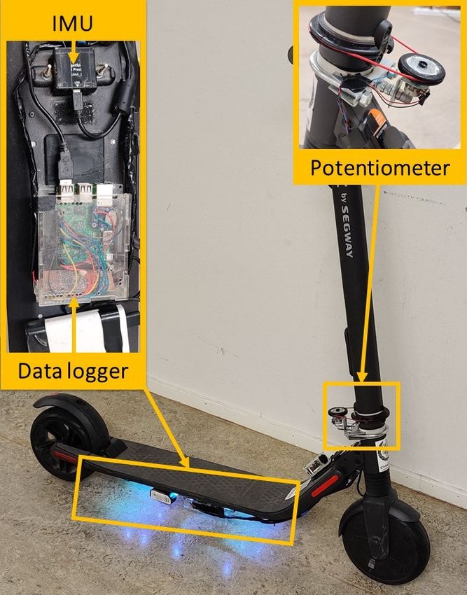
Contents
List of Figures xiii
List of Tables xv
1 Introduction 1
1.1 Background . . . . . . . . . . . . . . . . . . . . . . . . . . . . . . . . 1
1.2 Previous Research . . . . . . . . . . . . . . . . . . . . . . . . . . . . . 2
1.3 Research Question . . . . . . . . . . . . . . . . . . . . . . . . . . . . 3
1.4 Purpose . . . . . . . . . . . . . . . . . . . . . . . . . . . . . . . . . . 3
1.5 Scope . . . . . . . . . . . . . . . . . . . . . . . . . . . . . . . . . . . 3
2 Methodology 5
2.1 Vehicle Selection . . . . . . . . . . . . . . . . . . . . . . . . . . . . . 5
2.1.1 E-bike . . . . . . . . . . . . . . . . . . . . . . . . . . . . . . . 5
2.1.2 E-scooter . . . . . . . . . . . . . . . . . . . . . . . . . . . . . 6
2.1.3 Segway . . . . . . . . . . . . . . . . . . . . . . . . . . . . . . . 7
2.2 Data Acquisition System . . . . . . . . . . . . . . . . . . . . . . . . . 7
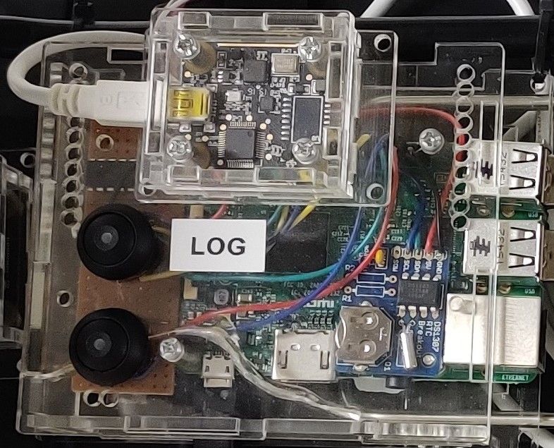
2.2.1 Data Logger . . . . . . . . . . . . . . . . . . . . . . . . . . . . 9
2.2.2 Inertial Measurement Unit . . . . . . . . . . . . . . . . . . . . 9
2.2.3 Steering Angle Sensor . . . . . . . . . . . . . . . . . . . . . . 10
2.2.4 LIDAR . . . . . . . . . . . . . . . . . . . . . . . . . . . . . . . 11
2.3 Participant Selection . . . . . . . . . . . . . . . . . . . . . . . . . . . 12
2.4 Experimental Protocol . . . . . . . . . . . . . . . . . . . . . . . . . . 13
2.4.1 Description of Tasks . . . . . . . . . . . . . . . . . . . . . . . 13
2.4.2 Set Up . . . . . . . . . . . . . . . . . . . . . . . . . . . . . . . 15
2.4.3 Main Experiment . . . . . . . . . . . . . . . . . . . . . . . . . 16
2.4.4 Questionnaire . . . . . . . . . . . . . . . . . . . . . . . . . . . 17
2.5 Performance Indicators . . . . . . . . . . . . . . . . . . . . . . . . . . 17
2.5.1 Speed . . . . . . . . . . . . . . . . . . . . . . . . . . . . . . . 21
2.5.2 Braking . . . . . . . . . . . . . . . . . . . . . . . . . . . . . . 21
2.5.3 Acceleration . . . . . . . . . . . . . . . . . . . . . . . . . . . . 21
2.5.4 Steering and Leaning . . . . . . . . . . . . . . . . . . . . . . . 21
2.5.4.1 E-bike, Bike and E-scooter . . . . . . . . . . . . . . . 21
2.5.4.2 Segway . . . . . . . . . . . . . . . . . . . . . . . . . 22
2.5.5 Box Plot . . . . . . . . . . . . . . . . . . . . . . . . . . . . . . 22
2.6 Data Analysis . . . . . . . . . . . . . . . . . . . . . . . . . . . . . . . 23
ixContents
2.6.1 Calibration . . . . . . . . . . . . . . . . . . . . . . . . . . . . 23
2.6.2 Post Processing . . . . . . . . . . . . . . . . . . . . . . . . . . 24
2.6.2.1 Syncing the Times . . . . . . . . . . . . . . . . . . . 24
2.6.2.2 Filtering . . . . . . . . . . . . . . . . . . . . . . . . . 24
2.6.2.3 Segmentation . . . . . . . . . . . . . . . . . . . . . . 25
2.6.2.4 Steering Angle Correction . . . . . . . . . . . . . . . 26
2.6.2.5 Orientation Estimation . . . . . . . . . . . . . . . . . 26
2.6.2.6 LIDAR Data Processing . . . . . . . . . . . . . . . . 26
2.6.2.7 Rauch-Tung-Striebel Smoother . . . . . . . . . . . . 27
3 Results 29
3.1 Data Overview . . . . . . . . . . . . . . . . . . . . . . . . . . . . . . 30
3.2 Performance Indicators . . . . . . . . . . . . . . . . . . . . . . . . . . 31
3.2.1 Speed . . . . . . . . . . . . . . . . . . . . . . . . . . . . . . . 31
3.2.2 Braking . . . . . . . . . . . . . . . . . . . . . . . . . . . . . . 33
3.2.3 Accelerating . . . . . . . . . . . . . . . . . . . . . . . . . . . . 37
3.2.4 Steering and Leaning . . . . . . . . . . . . . . . . . . . . . . . 39
3.2.4.1 E-bike, Bike and E-scooter . . . . . . . . . . . . . . . 39
3.2.4.2 Segway . . . . . . . . . . . . . . . . . . . . . . . . . 41
3.3 Questionnaire . . . . . . . . . . . . . . . . . . . . . . . . . . . . . . . 42
3.3.1 Mounting and Dismounting . . . . . . . . . . . . . . . . . . . 43
3.3.2 Accelerating from Standing Still . . . . . . . . . . . . . . . . . 43
3.3.3 Turning . . . . . . . . . . . . . . . . . . . . . . . . . . . . . . 44
3.3.4 Maintaining Low Speed . . . . . . . . . . . . . . . . . . . . . 44
3.3.5 Maintaining High Speed . . . . . . . . . . . . . . . . . . . . . 44
3.3.6 Keeping Balance . . . . . . . . . . . . . . . . . . . . . . . . . 44
3.3.7 Braking . . . . . . . . . . . . . . . . . . . . . . . . . . . . . . 45
3.3.8 Steering at Low Speed . . . . . . . . . . . . . . . . . . . . . . 45
3.3.9 Steering at High Speed . . . . . . . . . . . . . . . . . . . . . . 45
3.3.10 Overall . . . . . . . . . . . . . . . . . . . . . . . . . . . . . . . 45
4 Discussion 47
4.1 Data Analysis . . . . . . . . . . . . . . . . . . . . . . . . . . . . . . . 47
4.1.1 Speed . . . . . . . . . . . . . . . . . . . . . . . . . . . . . . . 47
4.1.2 Braking . . . . . . . . . . . . . . . . . . . . . . . . . . . . . . 47
4.1.3 Acceleration . . . . . . . . . . . . . . . . . . . . . . . . . . . . 48
4.1.4 Steering and Leaning . . . . . . . . . . . . . . . . . . . . . . . 49
4.1.5 Mounting and Dismounting . . . . . . . . . . . . . . . . . . . 50
4.2 Limitations . . . . . . . . . . . . . . . . . . . . . . . . . . . . . . . . 50
4.2.1 Data Sets Availability . . . . . . . . . . . . . . . . . . . . . . . 50
4.2.2 Potentiometer . . . . . . . . . . . . . . . . . . . . . . . . . . . 51
4.2.3 Measurement Uncertainty . . . . . . . . . . . . . . . . . . . . 51
4.2.4 Biases . . . . . . . . . . . . . . . . . . . . . . . . . . . . . . . 51
4.3 Future Work . . . . . . . . . . . . . . . . . . . . . . . . . . . . . . . . 52
5 Conclusion 53
xContents
A Data Set Availability I
B Questionnaire III
C Task Description Scripts IX
C.1 Script for E-bike, Bike and E-scooter . . . . . . . . . . . . . . . . . . IX
C.2 Script for Segway . . . . . . . . . . . . . . . . . . . . . . . . . . . . . X
xiContents xii
List of Figures
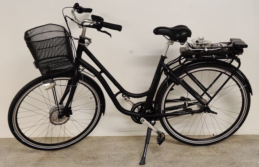
2.1 Monark Karin 3-VXL electric bike. . . . . . . . . . . . . . . . . . . . 5
2.2 Ninebot Kickscooter ES2. . . . . . . . . . . . . . . . . . . . . . . . . 6
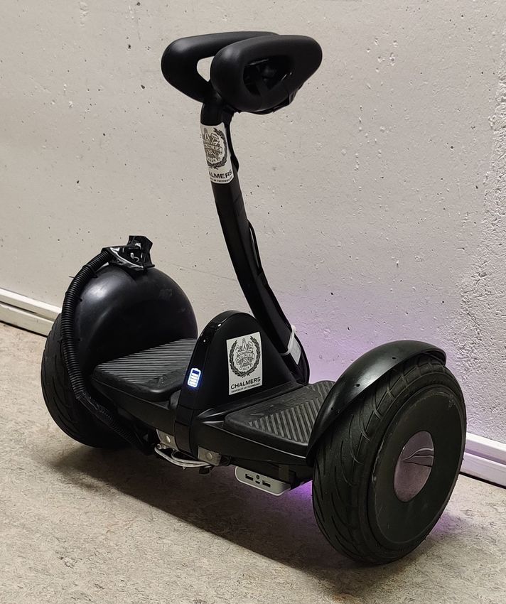
2.3 Segway Ninebot S. . . . . . . . . . . . . . . . . . . . . . . . . . . . . 7
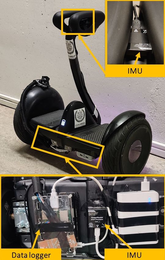
2.4 Vehicle instrumentation. . . . . . . . . . . . . . . . . . . . . . . . . . 8
2.5 Data logger which is mounted on the e-bike. On top of the data logger
is an IMU mounted. . . . . . . . . . . . . . . . . . . . . . . . . . . . 9
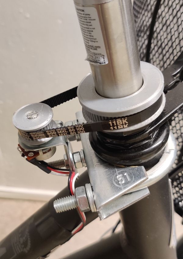
2.6 Steering angle sensor mounted on the steering stem of the e-bike and
e-scooter. . . . . . . . . . . . . . . . . . . . . . . . . . . . . . . . . . 10
2.7 IMU mounted on the top of the steering stick of the Segway. . . . . . 11
2.8 LIDAR mounted on a tripod. . . . . . . . . . . . . . . . . . . . . . . 12
2.9 The first task which is to study the behavior of constant high speed,
comfortable braking and comfortable acceleration. . . . . . . . . . . . 13
2.10 The second task which studies the behavior of constant high speed,
harsh braking and harsh acceleration. . . . . . . . . . . . . . . . . . . 14
2.11 The third task which studied the behavior of a harsh acceleration and
an unexpected harsh brake. . . . . . . . . . . . . . . . . . . . . . . . 14
2.12 The fourth task which studies the behavior during consecutive turns. 15
2.13 Illustration of the test area. . . . . . . . . . . . . . . . . . . . . . . . 15
2.14 Photo of the middle part of the test area. . . . . . . . . . . . . . . . . 16
2.15 Description of a box chart. . . . . . . . . . . . . . . . . . . . . . . . . 23
2.16 Process description for post processing. . . . . . . . . . . . . . . . . . 24
2.17 Example of the segmentation for the braking tasks. . . . . . . . . . . 25
2.18 An example of the segmentation for the slalom task. The origin is
the position of the LIDAR. . . . . . . . . . . . . . . . . . . . . . . . . 26
2.19 A speed estimate from the LIDAR, the accelerometer and the RTS-
smoother that uses both the LIDAR and the accelerometer. . . . . . 28
3.1 The age, height, weight and gender distributions of the participants
in the study. . . . . . . . . . . . . . . . . . . . . . . . . . . . . . . . . 29
3.2 Histograms of how often the participants use the different types of
vehicles. . . . . . . . . . . . . . . . . . . . . . . . . . . . . . . . . . . 30
3.3 A box chart showing the distributions of the participants average
speed in different segments where they were instructed to keep a con-
stant speed. . . . . . . . . . . . . . . . . . . . . . . . . . . . . . . . . 32
xiiiList of Figures
3.4 A box chart showing the distributions of the participants standard de-
viation of the speed in different segments where they were instructed
to keep a constant speed. . . . . . . . . . . . . . . . . . . . . . . . . . 32
3.5 Average speed across participants during gentle braking, harsh brak-
ing and unexpected braking with the four different vehicles. . . . . . 33
3.6 The braking trajectories for the harsh brake with the four different
vehicles. The origin is placed at the position of the LIDAR. . . . . . 34
3.7 The distributions for the mean braking distance and the mean longi-
tudinal acceleration for the braking segments. . . . . . . . . . . . . . 35
3.8 Box charts showing the distributions of the participants mean longi-
tudinal acceleration on the unexpected brake with the e-scooter and
the bike based on their experience. . . . . . . . . . . . . . . . . . . . 36
3.9 Box chart showing the distributions of the participants reaction time
in the unexpected task. . . . . . . . . . . . . . . . . . . . . . . . . . . 36
3.10 Average speed during gentle acceleration and harsh acceleration with
the four different vehicles. . . . . . . . . . . . . . . . . . . . . . . . . 37
3.11 A box chart showing the distributions of the participants mean lon-
gitudinal acceleration for the gentle, and harsh acceleration. . . . . . 37
3.12 A box chart showing the distributions of the participants mean abso-
lute lateral acceleration during the slalom segment. . . . . . . . . . . 38
3.13 Distributions of the mean absolute steering angle. . . . . . . . . . . . 39
3.14 Distributions of the mean absolute steering rate. . . . . . . . . . . . . 39
3.15 Distributions of the mean absolute roll angle. . . . . . . . . . . . . . 40
3.16 Distributions of the mean absolute roll rate. . . . . . . . . . . . . . . 40
3.17 Distributions of the correlations between roll rate and steering rate
in terms of linear fit and time delay. . . . . . . . . . . . . . . . . . . . 41
3.18 Average absolute pitch angle and pitch rate at high speed, low speed
and slalom with the Segway. . . . . . . . . . . . . . . . . . . . . . . . 41
3.19 Distribution of the mean absolute stick inclination rate with the Seg-
way during slalom. . . . . . . . . . . . . . . . . . . . . . . . . . . . . 42
3.20 A spider plot of the result of the questions about how the vehicles
performed when riding. The scale is converted from very poor, poor,
fair, good, very good, excellent and exceptional to 1-7 where 1 corre-
sponds to very poor and 7 to exceptional. . . . . . . . . . . . . . . . . 43
3.21 A spider plot of the overall questions of the vehicles performance.
The scale is converted from very poor, poor, fair, good, very good,
excellent and exceptional to 1-7 where 1 corresponds to very poor and
7 to exceptional. . . . . . . . . . . . . . . . . . . . . . . . . . . . . . 46
xivList of Tables
2.1 Technical specifications of PhidgetSpatial 3/3/3 1044_1B. . . . . . . 10
2.2 Performance indicators for bike, e-bike and e-scooter. Const, Acc
and Dec are abbreviations for constant, acceleration and deceleration.
S,M and C are abbreviations for stability, maneuverability and comfort. 19
2.3 Performance indicators for the Segway. Const, Acc and Dec are ab-
breviations for constant, acceleration and deceleration. S,M and C
are abbreviations for stability, maneuverability and comfort. . . . . . 20
3.1 Number of participants used for the different PIs. . . . . . . . . . . . 31
A.1 Data sets availability. Y indicating that the data is available and NX
means that the data is missing with problem ID X. N1 means that
the participant didn’t ride the vehicle, N2 means that LIDAR data is
missing for that vehicle and N3 means that the vehicle data is missing
for that vehicle. . . . . . . . . . . . . . . . . . . . . . . . . . . . . . . I
xvList of Tables xvi
1
                            Introduction

1.1      Background
In recent years, electric micro-mobility vehicles have increased in popularity dras-
tically [1, 2]. Micro-mobility vehicles refers to small, lightweight vehicles which
usually operates at a maximum of 25 km/h. The benefits of these vehicles are
their size, maneuverability, affordability and the existence of multiple ride-sharing
services. There are several different types of electric micro-mobility vehicles, for
example electric bike (e-bike), electric scooter (e-scooter), electric skateboard and
Segway.

The e-bike is one of the most common electric micro-mobility vehicles and it still
increases in popularity. According to Lee et al., bike makers and sellers are seeing
increases in sales of e-bikes [3]. They note that in Germany, e-bike sales in 2018 was
up by 36 percent compared to the previous year, which corresponds to nearly one
million e-bikes and in the first half of 2019 another million e-bikes were sold.

A different vehicle that has become very popular the last years is the electric scooter.
The increase in popularity of e-scooters has also led to more injuries. According to
Farley et al., the estimated visits due to e-scooter accidents in emergency depart-
ments in the US has increased from 4881 visits in 2014 to 29 628 visits in 2019
[4]. A major factor of the increase in popularity of e-scooters is due to ride-sharing
services that distributes the scooters in larger cities. This could be seen by reported
accidents in Stockholm where e-scooter companies started to rent out e-scooters in
2018 [5]. In 2018, only four accidents related to e-scooter were reported, while in
2019 (until 19 September), 150 accidents were reported [6].

An electric micro-mobility vehicle that differs a lot from e-scooter and e-bike is the
Segway. The Segway was invented in 1999 and was mostly used for tourist tours
and law enforcement [7]. However, its price was comparably high, which probably
is why the total sales of the original model, the Segway PT, were only 140 000 [8].
The movement of the Segway is controlled only by leaning which differs a lot from
for example e-bike and e-scooter [9].

In Sweden, to be classified as bikes, electric micro-mobility vehicles must have a
maximum speed of 20 km/h [10]. E-bikes are however an exception and are allowed
to assist with motor power up to 25 km/h. The characteristics of electric micro-

                                                                                      1
1. Introduction mobility vehicles are however often very different compared to a regular bike. A regular bike is for example self-stable at some speeds while this is never the case for the e-scooter [1]. Previous participant studies have shown that the e-scooter may be behind conventional bikes in braking capabilities [2, 11]. There is, however, no conclusive evidence from a larger amount of participants. 1.2 Previous Research This thesis is a continuation of Alessio Violin’s thesis from 2020 [11]. Violin de- veloped a data collection and data analysis procedure for comparing the safety of e-bikes, e-scooters and Segways in terms of stability, comfort and maneuverability. The data collection and analysis Violin did, were based on test data from eight dif- ferent persons. The conclusion drawn from his thesis was that the Segway was easy to maneuver at low speed but increased in difficulty as speed increased based on rider experience. The e-scooter was perceived by the participants almost as safe as the e-bike with a high maneuverability level and high comfort. Poor braking capa- bilities were the factor that made the e-scooter less safe than the e-bike. The e-bike was the most stable and comfortable in general but struggled a bit with lateral mo- tion and low speed maneuvering. A more extensive testing needs to be performed to validate the results. The goal of the study done by Garman et al. was to investigate the influence of the rider kinematics and vehicle dynamics on e-scooter stability [2]. They designed a test course to simulate an urban environment which required multiple maneuvers. The maneuvers were turning, slalom, acceleration, deceleration, stopping and unex- pected braking. A commercially available e-scooter instrumented with sensors was used to measure acceleration, velocity, steering angle, roll angle and GPS location. Out of the eight participants in the study, seven gave data that could be used for the analysis. The results show that when riding straight on a flat path the e-scooter show high levels of stability. During the low speed turning and slalom maneuver it was noted that the participants had to use counterbalance with their body to stabilize the vehicle. Results needs to be validated on a larger set of participants. A similar field experiment as the one performed during this thesis has been done be- fore by Kovácsová et al. [12]. They investigated cycling performance of middle-aged versus older participants during tasks where stabilization skills were important. In their study, they specifically looked at and compared conventional bikes and e-bikes. The authors came to the conclusion that cyclists rated themselves to be better than the average cyclists of the same age. Another conclusion that was drawn was that the participants’ self-reported cycling skills were different to the actual cycling per- formance. Participants had a lower roll rate while cycling at low speed with the e-bike than with the conventional bike which might indicate difficulties with stabi- lizing the vehicle. When participants were to ride at their own pace, they adopted a higher speed on the e-bike than the conventional bike. The participants reached the desired speed faster on the e-bike than on the conventional bike while accelerat- 2
1. Introduction

ing. This indicates that they need to exert more force on the conventional bike to
accelerate. This indicates a lower comfort for the regular bike than on the e-bike.

Miller et al. conducted an experiment to investigate the rider behavior of 20 Segway
operators: ten experienced operators and ten novices[13]. The experiment specif-
ically investigated the approach speed and clearance that Segway devices exhibit
on encountering a variety of obstacles on the sidewalk. They concluded that both
novice and experienced Segway riders were capable of traveling past the various ob-
stacles. Research containing more parameters regarding the safety of the Segway is
required in order to draw any conclusions regarding the general safety of the vehicle.

1.3      Research Question
The research question that was investigated in this thesis is:

      “How safe, in terms of stability, maneuverability and rider comfort, are
      e-bikes, e-scooters and Segways based on sensor data and user experi-
      ence?”

1.4      Purpose
The purpose of this thesis is to collect evidence for or against the safety level of
e-bikes, e-scooters and Segways in terms of stability, maneuverability and rider com-
fort.

1.5      Scope
There are plenty of electric personal mobility vehicles available, for example e-bikes,
e-scooters, Segways, electric skateboards, electric motorcycles and electric trikes just
to name a few. In this thesis only the first three, the e-bike, e-scooter and Segway,
are used in the evaluation of safety levels.

The participants included in the experiments conducted in this thesis are recruited
in the Gothenburg area, Sweden, and have to meet some inclusion criteria.

To ensure the safety of the participants the experiments are performed in an area
with little to none traffic and no hazardous tests are performed.

                                                                                      3
1. Introduction 4
2
                          Methodology

2.1     Vehicle Selection
Vehicle selection was made with a large influence from last year’s thesis by Alessio
Violin [11] since the vehicles used in his study were available and mounted with sen-
sors. The vehicles were chosen based on popularity, possibility of mounting sensors
and the ease of learning to ride.

2.1.1    E-bike
The chosen e-bike is a Monark Karin 3-VXL, shown in Figure 2.1, which is powered
by an EGOING-motor in the front wheel. The EGOING-motor helps the rider reach
a maximum speed of 25 km/h. This e-bike was chosen because of its ease of use and
it is an common model. Monark Karin 3-VXl has 5 different levels (1-5) of electric
assistance from the motor. The higher the level is, the higher the electric assistance
is. The e-bike is equipped with a coaster brake for the back wheel and a disc brake
for the front wheel.

Figure 2.1: Monark Karin 3-VXL electric bike.

                                                                                    5
2. Methodology As a reference, the e-bike was also used in the experiment as a conventional bike by turning off the electric assist by setting the assistance mode of the e-bike to 0. 2.1.2 E-scooter The e-scooter that was used is the Ninebot KickScooter ES2, shown in Figure 2.2. It has a maximum speed of 25 km/h. Although this is higher than 20 km/h which is the highest speed to be classified as a bike in Sweden, it is still a commonly used model. It has two levers on the handlebar, one for acceleration and one for brak- ing. There are three different power modes available on the Ninebot Kickscooter ES2. The three modes are sport mode, standard mode and speed limit mode. The sport mode gives the most power and speed but results in lower range while the speed limit mode gives the least power and speed but results in the longest range. The standard mode is in between the sport and speed limit mode. The e-scooter is equipped with an electric brake for the front wheel and a mechanical brake for the back wheel. The mechanical brake is integrated in the rear fender where the rider steps on it to initiate the brake. Figure 2.2: Ninebot Kickscooter ES2. 6
2. Methodology

2.1.3     Segway
The last electric micro-mobility vehicle that was examined was the Segway Ninebot
S, shown in Figure 2.3. According to Segway’s store, it is a smart self-balancing
electric transporter which is extremely portable, easy to learn and exciting to ride
[14]. It is not so common on the street, but is chosen due to its interesting balancing
and steering mechanism. The Segway Ninebot S has three different modes: sports
mode, new rider mode and safe mode with speed limits of 19, 10 and 7 km/h re-
spectively. By gently leaning forward and backward one controls the velocity of the
Segway Ninebot S. This model of the Segway does not have a handlebar. Instead,
the steering bar is located between the legs and to turn, one leans gently left or right
against the steering bar.

Figure 2.3: Segway Ninebot S.

2.2      Data Acquisition System
The vehicles were equipped with sensors to collect kinematics data. The sensors
mounted on the vehicles are Inertial Measurement Units (IMUs) and potentiome-
ters. The potentiometer was used to measure the steering angle and steering rate.
IMUs were used to be able to measure angular velocities and accelerations of the
vehicles. It was also used to estimate the orientation of the vehicles. The mount-
ing locations of the sensors can be seen in Figure 2.4. All three vehicles are also
equipped with a data logger which is used to record the sensor data.

                                                                                      7
2. Methodology (a) E-bike/bike (b) E-scooter (c) Segway Figure 2.4: Vehicle instrumentation. 8
2. Methodology

A light detection and ranging sensor (LIDAR) was used to track the planar motion
of the vehicles. During the experiments, the LIDAR was static and mounted on a
tripod, 80 cm above the ground, to the side of the test area. In order to get the best
view with the LIDAR it was placed in the middle of the 100-meter test track.

2.2.1      Data Logger
The data logger is the device logging the data coming from the different sensors.
The data logger is a Raspberry Pi 3 model B, which is a single-board computer
with a Quad Core 1.2GHz Broadcom BCM2837 64bit CPU and 1GB RAM, using
open-source software1 to save all the data to a USB memory stick. The open source
software is written in Python and uses the robotic operating system (ROS).

The data logger has two buttons, one for starting and stopping the recording of data
and the other one has two functions. While the data logger is recording data, the
second button works as a flag button meaning it gives an output of 1 when pressed
and 0 otherwise. The flag feature was used to synchronize the data signals with the
LIDAR’s data signals. The other function of the second button is to power off the
data logger completely which can only be done if the data logger is not recording
any data. The data logger can be seen in Figure 2.5.

Figure 2.5: Data logger which is mounted on the e-bike. On top of the data logger
is an IMU mounted.

2.2.2      Inertial Measurement Unit
The IMU used in this thesis was the PhidgetSpatial 3/3/3 1044_1B. An IMU is
used to measure acceleration, angular rates and magnetic field in three dimensions.
Technical specifications for the IMU can be seen in Table 2.1.

  1
      https://github.com/ruvigroup/div_datalogger

                                                                                    9
2. Methodology
Accelerometer
Acceleration measurement maximum range ±2.5g
Acceleration measurement resolution 76µg
Gyroscope
Gyroscope speed maximum range ±100◦ /s
Gyroscope resolution 0.0031◦ /s
Magnetometer
Magnetic field maximum range ±49.2G
Magnetometer resolution 1.5mG
Magnetometer noise 16mG
Table 2.1: Technical specifications of PhidgetSpatial 3/3/3 1044_1B.
2.2.3 Steering Angle Sensor
The e-scooter and the e-bike are both instrumented with a steering angle sensor
in the form of a potentiometer which can be seen in Figure 2.6. A belt system
connected to a wheel mounted on the potentiometer and the handlebar makes the
internal resistance of the potentiometer vary depending on the angle of the handle-
bar. An analog to digital converter (ADC) was used to measure the voltage across
the poles of the potentiometer, induced by the varying internal resistance. The volt-
age is then converted into steering angle by linear fitting. The ADC used was a 10
bit ADC connected to the Raspberry Pi through a serial peripheral interface (SPI)
connection.
(a) E-bike (b) E-scooter
Figure 2.6: Steering angle sensor mounted on the steering stem of the e-bike and
e-scooter.
102. Methodology
To convert the voltage from the potentiometer to a steering angle, a calibration
recording was made. The voltage was recorded when the handlebar was moved from
-30 degrees to 30 degrees in 5-degree steps where 0 degrees are when the handlebar is
straight. The linear function from the voltage to the corresponding angles that had
the least squared error was then used to convert voltage to degrees. This calibration
was made both for the e-scooter and e-bike.
Due to the lack of a handlebar on the Segway, no potentiometer was mounted. On
the Segway, the steering angle would compare to the stick inclination angle which
was measured using the IMU mounted on the top of the steering stick. The IMU
encased in a plastic case can be seen in Figure 2.7.
Figure 2.7: IMU mounted on the top of the steering stick of the Segway.
2.2.4 LIDAR
In order to record the motion of the vehicles, a LIDAR sensor was used. The LIDAR
used was the Hokuyo UXM-30LXH-EWA which has a guaranteed detection range of
30 m and a maximum detection range of 120 m. The LIDAR has a scanning angle
of 190° and an angular resolution of 0.125°. The logging platform for the LIDAR
was run on a Raspberry Pi 3 Model B implemented as a ROS package. The logging
software is the same as for the data loggers on the vehicles. A button was connected
to the Raspberry Pi which was used to synchronize the data from the LIDAR and
the vehicles. The button was also used to indicate when a maneuver started and
ended. To start the LIDAR, a web interface is used where you can either visualize
the LIDAR data in real time or record the data. The LIDAR mounted on a tripod
112. Methodology can be seen in Figure 2.8. Figure 2.8: LIDAR mounted on a tripod. 2.3 Participant Selection Participants that met the requirements in the list below were invited to the study. • Be at least 160 cm tall. • A maximum weight of 85 kg. • Be 18-50 years old. • Be able to ride a bicycle. • Do not have any physical disabilities. • Have not suffered from serious traffic accidents. • No symptoms of Covid-19 in the last two weeks before the study. The height criteria and the weight criteria were from limitations of the vehicles. The bicycle used was not suited for participants below 160 cm and the Segway had a maximum weight limit of 85 kg. The requirement, to be able to ride a bicycle, was set to have a good reference for the electric micro-mobility vehicles and to reduce the training time needed. The two requirements, not have any physical disabilities and not have suffered from serious traffic accidents were set primarily due to ethical concerns. The age limit was set to reduce the risks of injuries and to limit the number 12
2. Methodology

of between-subject factors. Apart from these requirements, a gender balance was
desired since both males and females use electric micro-mobility vehicles and could
potentially have different riding behaviors.

2.4      Experimental Protocol
All of the experiments with the participants were done on a pier located at Pump-
gatan 2 in Gothenburg, Sweden. The pier is a paved road for cyclists and pedestrians
with little to no traffic. This section will cover a description of the four tasks the
participants performed, how the test track was set up prior to participants arriving
at the scene as well as how the experiments were done in detail with each participant.

2.4.1     Description of Tasks
The participants performed four different tasks on each vehicle. The different ma-
neuvers that the participants performed are adapted from work by Kovácsová et al.
[12] and Rasch et al. [15].

Figure 2.9: The first task which is to study the behavior of constant high speed,
comfortable braking and comfortable acceleration.

The first task could be seen in Figure 2.9. It starts with the rider accelerating gently
until a speed between 17 km/h to 20 km/h has been reached and then continue in
the same speed before braking to stop before a line in a gentle way. Then acceler-
ating gently up to the interval 17-20 km/h again. This task was chosen to indicate
how the different vehicles behave in high speed, an expected braking situation and
accelerating. This is a common real life scenario when approaching a stop sign. A
small speed interval is set to give a fair comparison of the different vehicles, but
also make it easy for the rider to complete the task. The risk of setting an absolute
speed is that the rider gives a lot of attention to the speed monitor to not deviate
from the requested speed.

                                                                                     13
2. Methodology Figure 2.10: The second task which studies the behavior of constant high speed, harsh braking and harsh acceleration. The second task, which is the harsh maneuver, can be seen in Figure 2.10. It starts with the rider accelerating harshly to 17-20 km/h and maintaining that speed. The rider should then brake harshly and come to a complete stop before a line. Then they should proceed with accelerating harshly up to 17-20 km/h again and maintain that speed until they reach the finish line. In a real life scenario this could represent a person that perceives a stop signal too late due to not being attentive. This task also shows the braking and accelerating capabilities of the different vehicles. Figure 2.11: The third task which studied the behavior of a harsh acceleration and an unexpected harsh brake. The third task could be seen in Figure 2.11. It starts with accelerating to the interval 17-20 km/h. The rider then keeps a constant speed until it hears a sound signal, which is that one of the experimenters shouts stop. When the rider hears the sound signal they should brake harshly. This task represents an unexpected stop. In a real life scenario it is important to have a short braking distance to avoid a potential crash, but also that the braking is stable to avoid falling. 14
2. Methodology

Figure 2.12: The fourth task which studies the behavior during consecutive turns.

The fourth and final task is shown in Figure 2.12. Here the rider should accelerate to
7-10 km/h and try to maintain this speed while completing a slalom course around
four cones. Here the performance of the vehicles in turns are studied. This task
could represent passing obstacles or pedestrians in a real setting.

2.4.2    Set Up
Three lines were drawn on the ground using chalk to indicate start, brake and finish
locations. The start line is where all the tasks were started from and the finish line
is the end of the test track. The brake line is the line used in the gentle and harsh
maneuver to indicate where the participants should have come to a complete stop.
Four small cones were placed 3 meters apart, one by the brake line, two before the
brake line and one after the brake line. The LIDAR was positioned parallel to the
traffic cones aligned with the brake line to best capture the motion of the vehicles
in the most important part of the maneuvers which is acceleration, deceleration and
slalom. An illustration of the test area can be seen in Figure 2.13 and a photo of
the middle part of the test area can be seen in Figure 2.14.

Figure 2.13: Illustration of the test area.

                                                                                   15
2. Methodology Figure 2.14: Photo of the middle part of the test area. Before each participant arrived, the LIDAR was tested to see that it was aligned correctly and worked properly. Lamp posts on the pier was used to make sure the LIDAR was parallel to the road using the visualize function of the web application. To reduce the spread of COVID-19 the handlebars of the vehicles and the seat of the bike were disinfected and the experimenters had visors or protective masks. 2.4.3 Main Experiment When a participant arrived at the test location, a short introduction was given about the experiment. The participant was then asked to read through and sign a consent form. After the consent form was signed, the experimenter and the participant went through the experimental protocol together. When all the required information were given to the participant, they were equipped with a helmet and optional protectors for their knees, elbows and hands. The par- ticipants were then asked to try out all four vehicles (bike, e-bike, e-scooter and Segway). If any of the participants did not feel safe or felt uncomfortable riding any of the vehicles, that vehicle was skipped in the experiment. Same goes for the four different tasks. If any of the tasks felt uncomfortable for the participant, the task was skipped. After the participant had tried out all the vehicles, the main experiment could start. The order in which each of the participants were to ride each vehicle and task was randomized. This was done to reduce any potential learning effect. Before starting the tasks with each vehicle, there were some final set-up steps needed. The recording of the LIDAR and the data logger on the vehicle were started. When the recording of the on-board sensors on the vehicle, through the data logger, was started, the 16
2. Methodology

vehicle was kept in a stationary position for a couple of seconds. This was to give
the data logger enough time to calibrate the gyroscope. After the calibration was
done the flag button was pressed simultaneously on the data logger of the vehicle
and on the LIDAR to be able to sync the different sensors.

Before each task, the participant was given oral instructions on how to perform the
task which is shown in appendix C. The experimenter operating the LIDAR did a
short press on the flag button when the participant started each task and a long
press whenever the participant finished the task. For the unexpected task, a but-
ton press was also done whenever the signal was given to brake. For the e-bike,
a set electric assistance and mechanical gear was used for the different tasks. For
the slalom task the electric assistance was set to 2 and the mechanical gear was
set to 1. In the other three tasks, the electric assistance was set to 4 and the me-
chanical gear to 2. The e-scooter and Segway always had the highest power mode on.

After the participant had completed all the tasks with a vehicle, the data logger on
the vehicle and the LIDAR was stopped. Then the process restarted with starting
the data logger on the next vehicle and so on.

2.4.4     Questionnaire
When the participants were done with the riding tasks, they were asked to fill in a
questionnaire about their experience during the riding tasks as well as when they
tried out all the vehicles. The questionnaire can be seen in appendix B. It starts
with questions regarding the demographics and prior experiences of the participant.
It continues with questions about how they felt the different vehicles performed in 11
different scenarios. The questionnaire ends with four questions regarding the overall
comfort, maneuverability, stability and safety. All of the questions regarding the
performance of the vehicles and the overall questions are questions with a 7-grade
scale. The scale can be seen below:
   1. Very Poor
   2. Poor
   3. Fair
   4. Good
   5. Very Good
   6. Excellent
   7. Exceptional
After every question there is an optional field for adding comments. If the participant
chose not to ride any of the vehicles, the answers related to the skipped vehicles were
removed.

2.5      Performance Indicators
Performance indicators (PIs) are information collected at regular intervals to track
the performance of a system. In this thesis, a list of different PIs are being measured

                                                                                    17
2. Methodology and calculated in order to assess the safety of the e-vehicles in the dimensions sta- bility, maneuverability and rider comfort. A high stability indicates that the vehicle does not need a lot of correction by the user when riding. A high maneuverability indicates that the vehicle is easy to accelerate, decelerate and turn with. A high comfort indicates that the rider feels comfortable, does not need a lot of physical effort to maneuver the vehicle and is not subject to excessive force. The PIs are pa- rameters that can relate vehicle kinematics to one or more safety dimensions. Each task is split up into smaller segments. For the gentle and harsh maneuvers, there are three segments: 1) the constant seg- ment, 2) the acceleration segment and 3) the deceleration segment. The constant segment is the part of the task where the rider is trying to maintain a constant speed of 17-20 km/h. The constant segment will occur twice, both before the acceleration segment and after the deceleration segment. The slalom task is split up into two segments. The first segment is the constant seg- ment where the rider tries to maintain a constant speed of 7-10 km/h which occurs both before and after the slalom segment. The slalom segment is the part of the task where the rider is riding slalom around the traffic cones. In order to examine the reactions and braking capabilities during the unexpected task, it is split up into three segments. First, there is the constant segment where the rider tries to maintain a constant speed of 17-20 km/h. The second segment is the reaction segment which is from when the signal is given until the rider starts to brake. The third, and final segment, is the deceleration segment which is just like in the gentle and harsh maneuver the segment where the rider decelerates. The full list of PIs for the bike, e-bike and e-scooter can be seen in Table 2.2. The full list of PIs for the Segway can be seen in Table 2.3. 18
2. Methodology

 Signal                   Performance Indicator       Segment     Interpretation
                          Mean absolute steering
 Steering angle (deg)                                 Const,      S,M
                          angle
                                                      Slalom
                          Mean absolute steering
 Steering rate (deg/s)                                Const,      S
                          rate
                                                      Slalom
 Roll angle (deg)         Mean absolute roll angle    Const,      S
                                                      Slalom
 Roll rate (deg/s)        Mean absolute roll rate     Const,      S
                                                      Slalom
 Speed (km/h)             Mean speed                  Const,      M,C
                                                      Slalom
 Speed (km/h)             Standard deviation          Const,      M,C
                                                      Slalom
 Time (s)                 Time                        Acc, Dec,   M
                                                      Reaction
 Longitudinal             Mean
                                                      Acc, Dec    M,C
 acceleration (m/s2 )     longitudinal acceleration
 Lateral                  Mean absolute lateral
                                                      Slalom      C
 acceleration (m/s2 )     acceleration
 Distance (m)             Braking distance            Dec         M
 Steering rate (deg/s),
                          R2 of linear fit            Slalom      S
 Roll rate (deg/s)
 Steering rate (deg/s),   Time delay between roll
                                                      Slalom      M
 Roll rate (deg/s)        rate and steering rate

Table 2.2: Performance indicators for bike, e-bike and e-scooter. Const, Acc and
Dec are abbreviations for constant, acceleration and deceleration. S,M and C are
abbreviations for stability, maneuverability and comfort.

                                                                                 19
2. Methodology
Signal Performance Indicator Segment Interpretation
Stick inclination Mean absolute stick
Slalom S,M
rate (deg/s) inclination rate
Pitch angle (deg) Mean absolute pitch angle Const, C
Slalom
Pitch rate (deg/s) Mean absolute pitch rate Const, S
Slalom
Speed (km/h) Mean speed Const, M,C
Slalom
Speed (km/h) Standard deviation Const, S,M,C
Slalom
Time (s) Time Acc, Dec, M
Reaction
Longitudinal Mean longitudinal
Acc, Dec M,C
acceleration (m/s2 ) acceleration
Lateral Mean absolute lateral
Slalom C
acceleration (m/s2 ) acceleration
Distance (m) Braking distance Dec M
Table 2.3: Performance indicators for the Segway. Const, Acc and Dec are abbre-
viations for constant, acceleration and deceleration. S,M and C are abbreviations
for stability, maneuverability and comfort.
202. Methodology
2.5.1 Speed
The mean speed and the standard deviation of the speed are used as PIs for the
constant and slalom segment. A too low mean speed may indicate that the rider is
not comfortable enough to ride at a higher speed while a too high speed may indicate
that the rider has trouble with maneuvering the vehicle. The standard deviation of
the speed is a measurement of both maneuverability and comfort. If the standard
deviation of the speed is low it indicates that it is easy to keep a constant speed
which indicates a high maneuverability. It also indicates a high comfort since it
indicates that the user need to correct the speed less. For the Segway, the standard
deviation is also related to stability since trouble with balance will lead to changes
in speed.
2.5.2 Braking
The braking distance, the braking time and the mean longitudinal acceleration are
used as PIs for the deceleration segment. A short braking distance or time and a
high deceleration for the unexpected and harsh brake indicates that it is possible to
brake fast which indicates a high maneuverability. A high deceleration may however
also indicate less comfort.
The reaction time in the unexpected task is chosen as a PI to indicate maneuver-
ability since a high reaction time indicates that the rider needs more time to initiate
the braking.
2.5.3 Acceleration
The acceleration time and the mean longitudinal acceleration are used as PIs for
the acceleration segment. A short acceleration time and a high acceleration for the
harsh acceleration indicates that it is possible to accelerate fast which indicates a
high maneuverability. A high acceleration may however also indicate less comfort.
For the slalom segment the mean absolute lateral acceleration is used as a PI since
a high lateral acceleration may indicate less comfort.
2.5.4 Steering and Leaning
2.5.4.1 E-bike, Bike and E-scooter
The mean absolute steering angle, steering rate, roll angle and roll rate are used
as PIs for the constant and slalom segment. The peak cross-correlation between
steering rate and roll rate and the time delay between steering rate and roll rate are
used as PIs for the slalom segment. A high mean absolute steering angle, steering
rate, roll angle and roll rate indicates that the rider needs to do a lot of correction to
maneuver the vehicle, hence a low stability. For the slalom segment a low steering
angle also indicates high maneuverability since less steering is needed to pass the
cones. The peak cross-correlation between the steering rate and the roll rate shows
212. Methodology
how correlated the two control input from the rider are. A high correlation indicates
that the user have control of the maneuver and therefore high stability. A low
time delay between the roll rate and the steering rate indicates that the vehicle is
responsive, hence high maneuverability.
2.5.4.2 Segway
The pitch angle, pitch rate and the stick inclination rate are used as PIs for the
constant and slalom segment. The mean absolute pitch angle is related to comfort
since it may be less comfortable to lean forward than to stand in a upright position.
A high pitch rate may indicate that the rider does not have the stability to stand
in a stable way on the Segway. The same reasoning can be done for the standard
deviation of the speed. If the speed changes a lot it indicates that the posture
also changes a lot which may be a sign that the Segway is not stable. A low stick
inclination rate during the slalom may indicate that the rider does not need to do
fast correction to go through the slalom course and is therefore a sign of stability.
2.5.5 Box Plot
The PIs will mostly be presented in box charts that represent the distribution of
the data. A description of the box chart is shown in Figure 2.15 where the line
inside of the box is the sample median. The top and bottom edges of the box
are the upper and lower quartiles, respectively. Interquartile range (IQR) is the
distance between the upper and lower quartiles. The upper quartile corresponds
to the 0.75 quantile and the lower quartile corresponds to the 0.25 quantile. To
be classified as an outlier the value has to be more than 1.5 · IQR away from the
top or bottom of the box. Values that are outside the quartiles but not an outlier
are represented by the whiskers which in turn shows the nonoutlier maximum and
nonoutlier minimum. The notch is used to see the significance of difference of
medians. If notches of two boxes do not overlap, it means that they have different
medians at the 5% significance level. The significance level is based on a normal
distribution assumption, but can also be used to compare other distributions. If m
is the median and n is the number of data
√ points, the notch regions√top and bottom
edges correspond to m + (1.57 · IQR)/ n and m − (1.57 · IQR)/ n, respectively.
222. Methodology
Figure 2.15: Description of a box chart.
2.6 Data Analysis
2.6.1 Calibration
To be able to use the data from the IMUs to compute the PIs, the orientation with
respect to the vehicle needs to be known or estimated. The direction of the gravity
in the IMU frame is computed by collecting readings from the accelerometer, while
the vehicle is set in an upright position with the use of a level. From this a rotation
matrix that aligns the z-axis of the IMU with the vehicles vertical axis could be
computed by solving Equation (2.1), where g is the gravitational constant, R1 is the
rotation matrix and, ax , ay and az are the readings from the accelerometer.
0 ax
0 = R1 ay (2.1)
g az
The next step is to find the rotation matrix that aligns the x-axis of the IMU with the
lateral direction of the vehicle and the y-axis with the longitudinal direction. This
was done by leaning the vehicles such that the direction of the gravity is directed
only in the lateral and the vertical direction of the vehicle. The second rotation
matrix could then be computed from the rotated accelerometer reading by solving
Equation (2.2). In this equation k is an arbitrarily constant, R1 is the rotation
matrix from Equation (2.1), R2 is the second rotation matrix and, ax and ay are
readings from the accelerometer. By multiplying these two rotation matrices a rota-
tion matrix from the IMU frame to the vehicle frame was estimated. This rotation
232. Methodology
matrix was then applied to the acceleration readings from the accelerometer and the
angular velocity readings from the gyroscope.
0 ax
k = R2 R1 ay (2.2)
0 0
2.6.2 Post Processing
In order to be able to compute the PIs for the vehicles, the data collected during the
experiments needed to be processed. This section will cover the filtering methods
used, how the tasks were split up into the segments mentioned in Section 2.5, how
the orientation of the vehicles were estimated, and how the LIDAR data, together
with the IMU data, were used to estimate position and speed. The process of the
post processing can be seen in Figure 2.16.
Figure 2.16: Process description for post processing.
2.6.2.1 Syncing the Times
The data logger on the vehicles and the logging device on the LIDAR were instru-
mented with a real-time clock. The real-time clocks however suffered from drift over
time. All the logging devices had a connected flag button. Before starting the tests
with a vehicle, the button connected to the vehicle was pressed at the same time as
the button connected to the LIDAR.
For some participants, the syncing was not correct due to human errors and hard-
ware problems. The human errors were missing to press a button or not pressing
the buttons at the same time. Hardware problems was that the button press was
not registered due to loose wire connection. To sync the signals, the longitudinal
acceleration of the harsh task was derived from the LIDAR measurements. The
time lag between the LIDAR measurements and the IMU measurements was then
estimated with the finddelay function in MATLAB with the acceleration from the
LIDAR and the accelerometer of the IMU. The function finds the delay that gives
the highest cross correlation between the two signals.
2.6.2.2 Filtering
The steering angle, steering rate, angular velocity and orientation angles were all
filtered with a low-pass filter. The low-pass filter used was a zero-phase Butterworth
242. Methodology
filter [16] with a passband of 0-1 Hz and a stopband of 1-1.5 Hz.
2.6.2.3 Segmentation
The start and end of each maneuver were indicated by a flag button and could
therefore easily be extracted. Each maneuver also consists of different segments.
These are not indicated by any button press and instead based on the signal data.
The first segment of all the maneuvers is the constant segment which started after
the first 20 traveled meters, so that the rider had enough time to accelerate to the
given speed.
For the braking tasks, the next segment is the braking segment. It starts when going
under 16 km/h the last time before the stop for the bike, e-bike and the e-scooter
and ends when the speed is under 2.5 km/h. For the Segway, it starts when the
rider is going under 12 km/h the last time before the stop since the participant
had a lower speed with the Segway. The unexpected task ends after the stop, but
it also has a reaction segment which starts when the signal is shouted. After the
vehicle decelerates to a speed that is 1 km/h less than the speed at the time of
signal the reaction segment ends. For the gentle and harsh task, the third segment
is the acceleration segment which starts when the speed goes above 2.5 km/h and
ends at 16 km/h for e-bike, bike, and e-scooter, and 12 km/h for the Segway. After
that, a second constant segment starts which ends 10 meters before the finish line
to avoid collecting data from braking or steering that some participants did just
before the finish line. Examples of the segmentation for the braking tasks is shown
in Figure 2.17.
(a) Unexpected task. (b) Harsh/Gentle task.
Figure 2.17: Example of the segmentation for the braking tasks.
The slalom task is segmented solely based on position. After the first constant seg-
ment there is a slalom segment. The slalom segment starts 4 meters in front of
the first cone and ends 4 meters after the last cone. The second constant segment
starts directly after the slalom segment and ends 10 meter before the finish line. An
252. Methodology example of the segmentation for the slalom task is shown in Figure 2.18. Figure 2.18: An example of the segmentation for the slalom task. The origin is the position of the LIDAR. 2.6.2.4 Steering Angle Correction A mean correction of the steering angle was made for each maneuver to correct for potential drift. During the constant segment it was assumed that the mean steer angle was zero. The mean steer angle of the constant segment was therefore removed from the steer angle measurements for each task. 2.6.2.5 Orientation Estimation The orientation of the vehicles was estimated by using a Madgwick filter [17] with the measurements from the gyroscope and accelerometer. The magnetometer values were not used since the values were heavily affected by disturbances, even after calibration. This is probably due to soft iron disturbances from the electronics on the vehicle which is very hard to compensate for. The magnetometer is also mostly used for the yaw angle estimate which could be estimated from the LIDAR measurements instead. 2.6.2.6 LIDAR Data Processing The LIDAR data consist of a set of 2D points. To extract the position of the vehicle, the LIDAR data were clustered. The detected view was limited to the test area to avoid potential clusters from the environment. The limits were set to ±50 meters in the longitudinal direction, and between two and nine meters in the lateral direction, where the position of the LIDAR is placed at the origin. The clustering method that was used was DBSCAN which is a clustering algorithm that clusters 26
2. Methodology
data based on the density and can discover clusters of arbitrary shape [18]. The
center of the cluster representing the vehicle was then interpreted as the center of
the vehicle. A first estimate of the speed of the vehicle was then estimated from the
LIDAR data by measuring the change of position of the cluster center over time.
A better estimation of the speed was then computed by fusing the estimation from
the LIDAR with the accelerometer data.
2.6.2.7 Rauch-Tung-Striebel Smoother
The Rauch-Tung-Striebel (RTS) smoother [19] was used to estimate the position and
the speed of the rider. For the gentle, harsh and unexpected task, there should be
no turning and therefore a one-dimensional model was used. The prediction model
is shown in (2.3) where the distance (d) and speed (v) represent the state vector and
the longitudinal acceleration (a) from the accelerometer on the vehicle is the input.
The sampling period is denoted as T . The measurement model is shown in (2.4)
and uses the distance (DL ) and speed (VL ) acquired from the LIDAR measurements.
2
" # " #" # " #
T
dk 1 T dk−1
= + 2 ak + Q1 (2.3)
vk 0 1 vk−1 T
" # " #" #
DL,k 1 0 dk
= + R1 (2.4)
VL,k 0 1 vk
In the slalom task, the rider turns and therefore a two-dimensional model was used.
The prediction model for the slalom task is shown in (2.5) where the state vector
includes the position (x, y), the linear speed (v) and the heading (φ). The position
of the LIDAR is set to the origin. The position in the longitudinal direction of the
track is described with x. The position in the lateral direction is described with y.
The longitudinal acceleration (a) from the accelerometer and the yaw rate (ω) from
the gyroscope are treated as inputs. The sampling period is denoted as T . The
measurement model for the slalom model is shown in (2.6) and uses the position
(XL , YL ) and speed (VL ) acquired from the LIDAR measurements.
xk 1 0 T cos(φk−1 ) −T vk−1 sin(φk−1 ) 0 0 " #
y 0 1 T sin(φk−1 ) T vk−1 cos(φk−1 ) 0 0
ak
k
= + + Q2 (2.5)
vk 0 0 1 0 T 0 ωk
φk 0 0 0 1 0 T
x
1 0 0 0 k
XL,k
yk
YL,k = 0 1 0 0 + R2 (2.6)
vk
VL,k 0 0 1 0
φk
Q and R are matrices that describe the noise. Q represents the uncertainty of the
prediction model and R represents the insecurity of the measurements. These ma-
trices were tuned to give a stable result and are shown in (2.7) and (2.8) where σ
was set to 10 for the Segway and 1 for the other vehicles. The sampling period is
27You can also read