Experimental Evaluation of Computer Vision and Machine Learning-Based UAV Detection and Ranging - MDPI
←
→
Page content transcription
If your browser does not render page correctly, please read the page content below
drones

Article
Experimental Evaluation of Computer Vision and Machine
Learning-Based UAV Detection and Ranging
Bingsheng Wei †,‡ and Martin Barczyk *,†,‡

                                          Department of Mechanical Engineering, University of Alberta, Edmonton, AB T6G 1H9, Canada;
                                          bingshen@ualberta.ca
                                          * Correspondence: mbarczyk@ualberta.ca
                                          † Current address: Department of Mechanical Engineering, University of Alberta,
                                            Edmonton, AB T6G 1H9, Canada.
                                          ‡ These authors contributed equally to this work.

                                          Abstract: We consider the problem of vision-based detection and ranging of a target UAV using
                                          the video feed from a monocular camera onboard a pursuer UAV. Our previously published work
                                          in this area employed a cascade classifier algorithm to locate the target UAV, which was found
                                          to perform poorly in complex background scenes. We thus study the replacement of the cascade
                                          classifier algorithm with newer machine learning-based object detection algorithms. Five candidate
                                          algorithms are implemented and quantitatively tested in terms of their efficiency (measured as frames
                                          per second processing rate), accuracy (measured as the root mean squared error between ground
                                          truth and detected location), and consistency (measured as mean average precision) in a variety of
                                          flight patterns, backgrounds, and test conditions. Assigning relative weights of 20%, 40% and 40% to

                                          these three criteria, we find that when flying over a white background, the top three performers are
                                   YOLO v2 (76.73 out of 100), Faster RCNN v2 (63.65 out of 100), and Tiny YOLO (59.50 out of 100),
Citation: Wei, B.; Barczyk, M.            while over a realistic background, the top three performers are Faster RCNN v2 (54.35 out of 100, SSD
Experimental Evaluation of                MobileNet v1 (51.68 out of 100) and SSD Inception v2 (50.72 out of 100), leading us to recommend
Computer Vision and Machine               Faster RCNN v2 as the recommended solution. We then provide a roadmap for further work in
Learning-Based UAV Detection and          integrating the object detector into our vision-based UAV tracking system.
Ranging. Drones 2021, 5, 37. https://
doi.org/10.3390/drones5020037             Keywords: UAVs; computer vision; detection; machine learning; neural networks; CNN; Tensor-
                                          Flow; darknet
Academic Editor: Pablo
Rodríguez-Gonzálvez

Received: 8 April 2021
                                          1. Introduction
Accepted: 3 May 2021
Published: 9 May 2021
                                                Human beings can easily detect and track objects using their eyes. The human brain
                                          can differentiate between various kinds of an object, e.g., different animal species. Studying
Publisher’s Note: MDPI stays neutral
                                          how computers can mimic human perception can be traced as far back as 1966, when an
with regard to jurisdictional claims in
                                          undergraduate student at Massachusetts Institute of Technology was asked to program
published maps and institutional affil-
                                          a computer to recognize what it saw from a camera [1]. Today, computer vision and
iations.                                  perception is widely deployed in areas such as manufacturing, terrain surveying, robot
                                          navigation, and many others.
                                                A well-known computer vision algorithm for object detection is the Cascade Classi-
                                          fier [2,3], originally developed to detect human faces in video streams. Due to its popularity,
                                          this algorithm is included in the OpenCV [4] library. The Cascade Classifier was notable for
Copyright: © 2021 by the authors.
Licensee MDPI, Basel, Switzerland.
                                          being one of the first algorithms to employ an offline training step prior to the online detec-
This article is an open access article
                                          tion step. This algorithm was employed in [5] for the purpose of detecting and following a
distributed under the terms and
                                          target UAV by a pursuing UAV equipped with an on-board monocular camera. While the
conditions of the Creative Commons        system was experimentally validated to work, the Cascade Classifier was found to be poor
Attribution (CC BY) license (https://     at detecting objects in conditions different from the training dataset. For example, if the
creativecommons.org/licenses/by/          algorithm was trained using pictures of the drone hovering over a white background, it
4.0/).

Drones 2021, 5, 37. https://doi.org/10.3390/drones5020037                                                 https://www.mdpi.com/journal/drones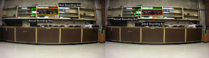
Drones 2021, 5, 37                                                                                            2 of 26

                     had difficulties detecting the same drone performing maneuvers involving large tilt angles
                     or flying over complex (non-white) backgrounds.
                           A newer approach to vision-based object detection are machine learning-based neural
                     networks, inspired by the structure of the human brain. A milestone event for this approach
                     was AlexNet winning the ImageNet Large Scale Visual Recognition Challenge (ILSVRC)
                     in 2012 [6]. Machine learning methods are more powerful than classifier-based detection
                     methods, e.g., while a classifier-based method can detect dogs in a picture, a machine
                     learning method can additionally identify the species of each dog it detects. Machine
                     learning training and detection each require performing enormous amounts of computa-
                     tions. Thanks to recent advances in computer hardware, specifically Graphics Processing
                     Units (GPUs) enabling massive parallelization of calculations, it is now feasible to perform
                     training using standard desktop-class computers and perform the detection process in
                     real-time on video streams.
                           This article presents work performed on the implementation and benchmarking of
                     various machine learning algorithms for the task of detection and ranging of a target UAV
                     using the video feed from a monocular camera equipped onboard a pursuer UAV. We
                     have deemed a vision-based sensing solution to be superior to conventional UAV detection
                     technologies such as acoustic [7] or radar [8], since the latter are best suited for being
                     installed on the ground due to their much higher weight and power draw relative to
                     monocular cameras. The specific contribution is to provide a detailed set of benchmarks of
                     the performance of these methods in a wide variety of flight patterns and under different
                     test conditions, quantifying the ranging performance using an optical motion-capture
                     system installed in our flight arena and making a recommendation about the choice of
                     algorithm based on these results. While other studies have been published regarding
                     testing and benchmarking of vision-based UAV detection and ranging, for instance [9–11],
                     our study is unique in combining a broad choice of object detection algorithms (five
                     candidates), having access to exact ground truth provided by an indoor motion capture
                     system, and employing the commercial Parrot AR.Drone 2.0 UAV which brings about the
                     challenges of its difficult-to-spot frontal profile due to its protective styrofoam hull and the
                     low-resolution video from its onboard camera. We have chosen to focus exclusively on
                     the case of the camera being carried onboard the pursuer UAV, as opposed to one or more
                     camera on the ground, since this aligns with our lab’s focus on vision-based UAV-to-UAV
                     pursuit as a multi-faceted research program blending techniques from computer vision,
                     state estimation, and control systems.
                           The remainder of this paper is structured as follows. Section 2 provides a background
                     for machine learning algorithms and current implementations, then covers our methodol-
                     ogy for quantifying the performance of vision-based detection and ranging of the target
                     UAV. Section 3 covers the training process of the object detection systems, where a series
                     of manually labeled images of the UAV are used to train the system to perform detection
                     on previously unseen images. Section 4 covers the benchmarking of the trained object
                     detection systems under a set of different flight patterns and test conditions, quantifying
                     the resulting performance in terms of efficiency, accuracy, and consistency, ending with a
                     recommendation for the choice of object detection system based on the numbers obtained.
                     Section 4.4 summarizes the paper and provides recommendations for further work.

                     2. Background and Methodology
                          Thanks to the ongoing development of Artificial Intelligence (AI), the method of
                     machine learning has brought in new approaches to computer vision-based object detection
                     such as artificial neural networks. Various machine learning frameworks are now publicly
                     available including TensorFlow, Caffe, Keras, Darknet, etc. Good support and frequent
                     updates from Google have made TensorFlow today’s most popular machine learning
                     framework [12].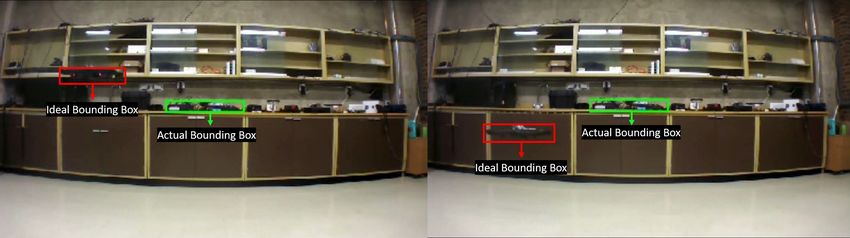
Drones 2021, 5, 37                                                                                           3 of 26

                          This section introduces specific object detection systems including Single Shot multi-
                     box Detector (SSD) and Faster Region-based Convolutional Neural Network (Faster RCNN)
                     which run under TensorFlow and You Only Look Once (YOLO) which runs under Darknet.
                     We then cover metrics used to quantify the precision of object detection, equations to range
                     the target UAV from a monocular camera video feed, the process of camera calibration,
                     and the testing methodology used in the following sections.

                     2.1. TensorFlow
                          TensorFlow is an open source software library for machine learning developed by
                     Google based on DistBelief, a closed-source machine learning framework [13]. “Tensor”
                     stands for multidimensional data and “Flow” stands for the manner of processing this
                     data. TensorFlow runs a number of publicly available object detection systems. We will
                     use and benchmark three of these: Single Shot multibox Detector (SSD) MobileNet v1,
                     SSD inception v2, and Faster Region-based Convolutional Neural Network (Faster RCNN).
                     Details of these are provided below.

                     2.1.1. Single Shot Multibox Detector (SSD)
                          Single Shot multibox Detector was proposed in [14]. SSD employs a base feed-forward
                     convolutional network to produce an initial collection of bounding boxes and their as-
                     sociated detection probabilities, followed by a set of convolutional feature layers which
                     progressively decrease in size and allow predictions at multiple scales.

                     2.1.2. Inception
                          Inception v1 is a detection architecture proposed in [15]. The original design, Inception
                     v1, consists of two models: a “Naive” model and a dimension-reducing model. The “Naive”
                     model contains three filters and a max pooling layer. However, this architecture was
                     inefficient and required an excessive amount of computation power. Extra convolutions
                     were thus added before the filters and after the max pooling layer. This reduces the
                     dimension of the input to enhance computational efficiency [15].
                          In order to improve detection accuracy and speed, Inception v2 was introduced in [16].
                     The architecture consists of a series of convolution steps, followed by Inception modules
                     and a pooling filter bank leading to classification. The overall architecture is 42 layers deep
                     and provided superior performance relative to other architectures [16].

                     2.1.3. MobileNet
                          MobileNet is a CNN architecture proposed in [17] optimized for low-power mobile
                     and embedded vision applications. MobileNet employs depthwise separable convolutions,
                     consisting of a separate layer for filtering and a separate layer for combining. This ap-
                     proach reduces both computation and model size relative to a standard convolution, with
                     negligible loss in accuracy [17].

                     2.1.4. Faster Region-Based Convolutional Neural Network (Faster RCNN)
                          Regions with CNN features (RCNN) was proposed in [18]. RCNN first extracts region
                     proposals from the input image, extracts a feature vector from each region using a CNN,
                     then scores each feature using its corresponding Support Vector Machine (SVM) [18]. This
                     yields excellent accuracy but requires around 10 seconds to process an image [18], making
                     it unusable for real-time video processing.
                          Fast RCNN [19] is an extension of RCNN. Instead of running each region proposal
                     through a CNN, the input image is run through several convolutional and max pooling
                     layers to produce a convolutional feature map. Then, for each region proposal a pooling
                     layer extracts a feature from the feature map, meaning feature extraction is done only once.
                     Each feature is then passed to a sequence of fully connected layers which yield classification
                     probability and bounding box estimates using softmax layers for objects. Image processing
                     speed for Fast RCNN was benchmarked to be 146 times faster than RCNN [19].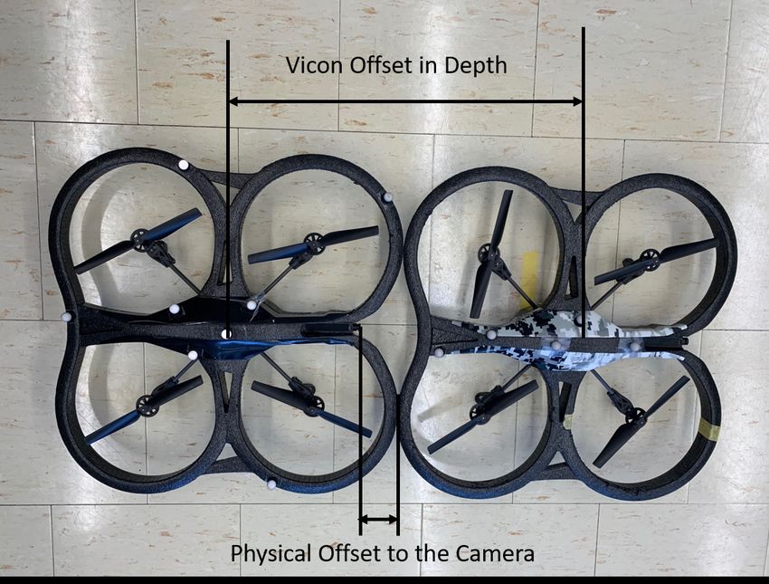
Drones 2021, 5, 37                                                                                           4 of 26

                          Faster RCNN was proposed in [20] with the goal of further optimizing the speed of
                     Fast RCNN. Faster RCNN works by employing Region Proposal Networks (RPN), a CNN
                     which produces region proposals, to replace selective search algorithm in Fast RCNN. In
                     this way the region proposal step can be carried out in around 10 ms, allowing real-time
                     object detection for the overall pipeline. Runtime speed of Faster RCNN was found to be
                     roughly ten times faster than Fast RCNN [20].

                     2.2. Darknet
                          Darknet is an open source machine learning framework written in C language and
                     CUDA [21]. Darknet is faster than TensorFlow in specific tasks, for instance object detection,
                     as shown in Section 4.1. This is important for running on single-board computers which
                     have a limited power budget.
                          The object detection models You Only Look Once (YOLO) and Tiny YOLO are trained,
                     tested, and benchmarked within Darknet.

                     You Only Look Once (YOLO)
                           You Only Look Once was introduced in [22]. YOLO employs an end-to-end single
                     neural network to reframe the classification problem into a regression problem which
                     predicts bounding boxes and their associated probabilities in one evaluation pass to avoid
                     complex pipeline [22].
                           Tiny YOLO, also known as Fast YOLO, was also proposed in [22] and employs fewer
                     convolutional layers (9 versus 24) and fewer filters within these layers to achieve faster
                     performance, with an associated reduction in detection accuracy. The implementation
                     details are otherwise identical to YOLO.
                           YOLO v2 is a newer version of YOLO which increases detection accuracy as well as
                     efficiency [23]. YOLO v2 employs batch normalization, trains the classification network
                     with higher-resolution images, uses anchor boxes to predict bounding boxes, finds good
                     priors in the training dataset by using k-means clustering on the bounding boxes, predicts
                     box location coordinates relative to grid cells, concatenates low and high resolution features
                     for the detector, and trains the network with a range of input image dimensions to make
                     it capable of using a wide range of input resolutions. These features contribute to an
                     improvement in detection performance.

                     2.3. Detection Precision Metrics
                         The performance of object detection systems such as Faster RCNN and YOLO are
                     measured using mean Average Precision (mAP). The calculation of mAP relies on recall
                     and precision, which are discussed below.

                     2.3.1. Intersection over Union (IoU)
                          Intersection over Union (IoU) measures the quality of the bounding box of a detected
                     object. An example of a detected UAV bounding box is shown in Figure 1.
                          The ground truth is the exact boundary of the object. The bounding box is the rectangle
                     estimated by the detection system. IoU is then calculated as
                                                                      T
                                                Ground Truth Area Bounding Box Area
                                          IoU =                  S
                                                Ground Truth Area Bounding Box Area
                          In this paper, bounding boxes with an IoU of 0.5 or more are considered to be a
                     positive detection.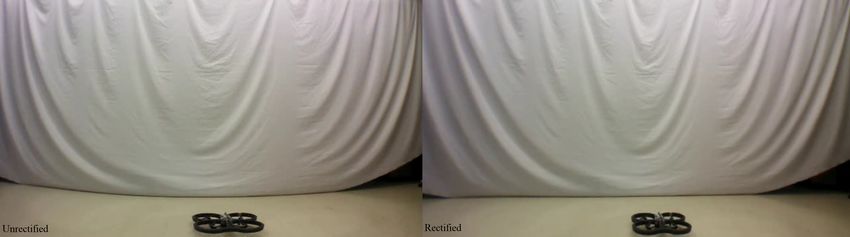
Drones 2021, 5, 37                                                                                         5 of 26

                     Figure 1. Ground Truth and Bounding Box.

                     2.3.2. Recall and Precision
                          Recall describes the rate of detecting objects in an image. Precision describes the
                     accuracy of these positive detections. Figure 2 illustrates the possible classifications of
                     detected items.

                     Figure 2. Classification of Items in a Detection.

                          Recall and precision are calculated as

                                                                         DC
                                                               Recall =
                                                                       DC + UC
                                                                         DC
                                                           Precision =
                                                                       DC + DI
                          The larger the recall and precision, the more accurate the detection.

                     2.3.3. Average Precision (AP) and Mean Average Precision (mAP)
                          Both recall and precision need to be considered when measuring the accuracy of a
                     detection system. Average Precision (AP) is the area under the precision-recall curve. AP is
                     calculated as
                                                                         n
                                                              AP =   ∑ p(i)∆r(i)
                                                                     i =1

                     where p(i ) is the precision at each detection and ∆r (i ) is the recall difference between
                     detection i − 1 and i.
Drones 2021, 5, 37                                                                                             6 of 26

                         Mean Average Precision (mAP) takes an average over different detection sets and thus
                     measures the overall accuracy of the object detection system. mAP is calculated as
                                                                           n
                                                                      1
                                                          mAP =
                                                                      n   ∑ AP(i)
                                                                          i =1

                     where n is the number of detection sets, and AP(i ) is the average precision at each set.
                          Note mAP only reflects the rate of correctly detected objects in a set of data, and it
                     does not quantify the difference in dimensions between a detected bounding box and
                     the ground truth (the exact size of the bounding box). The dimensions of the bounding
                     box are used to estimate the distance of the target UAV from the pursuer, as explained in
                     Section 2.4.

                     2.4. Distance Estimation from a Monocular Camera
                          Depth-sensing cameras such as the Kinect [24] have the ability to directly measure
                     3D images. However, our UAV’s onboard camera is monocular and can only capture 2D
                     images. In order to track a UAV, its 3D position relative to the follower must be estimated
                     using the method described in this section. In order to verify the accuracy of the calculated
                     depth, the estimated results will be compared against a ground truth provided by a Vicon
                     motion capture system installed in our lab.
                          We model the monocular camera by the well-known pinhole camera model shown in
                     Figure 3, which assumes the aperture of the lens approaches zero, such that the only ray
                     from a point p passing to the image plane is the one through the optical center of the lens.
                     The focal length f > 0 is the distance from the lens to the imaging plane. Figure 3 introduces
                     the camera lens-fixed reference frame C whose origin is placed at the optical center of the
                     lens, as well as a frame I on the image plane whose origin lies at the intersection of the
                     optical axis with the image plane.
                               e
                            an

                                                                                 p
                          Pl

                                        Optical center
                          e
                      ag
                     Im

                           I              C
                                               c3                                Optical axis
                      i1 i         c1     c2
                          2
                       p0

                                   f
                     Figure 3. Pinhole camera model.

                          Within Figure 3 let ( X, Y, Z ) denote the coordinates of p w.r.t. frame C, and let ( x, y)
                     denote the coordinates of the corresponding point image p0 w.r.t. frame I. Using similar
                     triangles provides the relationships

                                                                X                       Y
                                                       x = −f     ,            y = −f     .                       (1)
                                                                Z                       Z
                           The negative signs above reflect the fact that the image projected onto the image
                     plane, which in a digital camera corresponds to the CCD sensor array, is an upside-down,
                     mirror-flipped version of the scene in front of the camera. This is intrinsically compensated
                     for in the firmware of the camera, such that the reported image correctly renders the scene.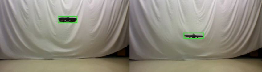
Drones 2021, 5, 37 7 of 26
For this reason, we can remove the negative signs in (1). Using homogeneous coordinates,
we thus express the mapping (1) from the 3D point ( X, Y, Z ) to 2D point ( x, y) as
X
x f X/Z X f 0 0 0
y = f Y/Z = f Y = 1 0 f 0 0
Y
Z Z Z
1 1 Z/ f 0 0 1 0
1
(2)
X
f 0 0 1 0 0 0
1 Y
= 0 f 0 0 1 0 0
Z
Z
0 0 1 0 0 1 0
| {z }| {z } 1
Kf Π0
The model above is entirely in SI units of length, namely ( X, Y, Z ), f , and ( x, y) are all
given in units of m. However, since we are using a digital camera, we need to transform
( x, y) into coordinates ( x 0 , y0 ), which are in units of pixels (px), and whose origin is at the
top-left of the image. This transformation is done in two steps. First, the dimensions in m
are transformed into px as
xs = s x x
ys = sy y
where s x , sy in units of px/m are scaling factors; if s x = sy the pixels are square, but this is
not always the case. The scaled coordinates are then transformed into the digital image
frame as
x 0 = xs + c x
y0 = ys + cy
where (c x , cy ) are the coordinates of the optical axis with respect to the digital image frame,
in units of px. The two transformations combine to
0
x sx 0 cx x
y0 = 0 sy cy y
1 0 0 1 1
| {z }
Ks
Returning to (2) and left-multiplying both sides by Ks gives:
0 X
x sx f 0 cx 1 0 0 0
y0 = 1 0 sy f c y 0 1 0 0
Y
(3)
Z Z
1 0 0 1 0 0 1 0
| {z }| {z } 1
K Π0
where K is known as the intrinsic camera matrix, whose entries are determined by the
optics of the camera and are fixed. Note both s x f := f x and sy f := f y are in units of px.
Matrix K is upper-triangular, and so it has an inverse since all of its diagonal entries are
non-zero. Based on (3) we also define the projection matrix P := KΠ0 , such that
fx 0 cx 0
P = 0 fy cy 0 (4)
0 0 1 0
Estimating the target UAV’s position from monocular camera images can be done
under the following assumptions:Drones 2021, 5, 37 8 of 26
• The detection method provides accurate rectangular bounding boxes around the
target UAV
• The physical dimensions of the target UAV are precisely known
• The target’s visible width and height do not change much during the experiment
The first two assumptions are reasonable. The third one is much more restrictive
and requires the target UAV to maintain its yaw angle relative to the pursuer as close to
zero and not to fly too much above or below the pursuer. For instance, our UAV has a
width and depth of 52 cm and a height of 13 cm. When it faces away from the follower, its
visible width and height are known to be 52 cm by 13 cm. However, if it yaws by 45◦ , its
visible width changes to (522 + 522 )1/2 = 73.5 cm—a 41% increase—which violates the
third assumption. One approach to removing this assumption would be to train the CNN
to classify different orientations of the target UAV and use this information to dynamically
assign a visible width and height.
Expanding (3) yields the following two relations:
X
x0 = f x + cx
Z (5)
Y
y0 = f y + cy
Z
0 , y 0 , x 0 , y 0 ),
The CNN provides rectangular bounding boxes in the form of a vector ( xul ul dr dr
0 0
where ( xul , yul ) are the digital image frame coordinates of the upper-left corner and
0 , y0 ) are those of the lower-right, all in units of px. The width of the bounding box
( xdr dr
is thus w0 = xdr 0 − x 0 . Let X and X denote the camera lens-fixed frame C coordinates
ul ul dr
of the points in 3D space corresponding to the upper-left and bottom-right pixel of the
bounding box, and let Z denote their common depth. Under the earlier assumption that
the target has a near-zero yaw angle, Z physically represents the perpendicular distance
between the follower’s camera and the target’s rear face. We have
w0 = xdr
0 0
− xul
Xdr X
= fx + c x − f x ul + c x
Z Z
fx
w0 = ( X − Xul )
Z dr
However, Xdr − Xul := W is the true visible width of the target UAV, which is known.
Thus we can solve for the depth (of the rear surface of the UAV) as
fxW
Zw = (6)
w0
Note this Zw is calculated using only width information. Using the same procedure
with height h0 = y0dr − y0ul of the bounding box, we have
h0 = y0dr − y0ul
Ydr Yul
= fy + cy − f y + cy
Z Z
fy
h0 = (Ydr − Yul )
Z
and with Xdr − Xul := H known as the true visible height of the target UAV, we get
fy H
Zh = (7)
h0Drones 2021, 5, 37 9 of 26
The results from (6) and (7) should be identical. In practice, errors in the bounding
box estimated dimensions w0 and h0 will affect the computed Z. To mitigate this we take
the average of the quantities as
Zw + Zh f x h0 W + f y w0 H
Z= = (8)
2 2w0 h0
Knowing Z, we proceed as follows: inverting (5), we obtain
X x0 − cx Y y0 − cy
= =
Z fx Z fy
We find the digital image frame coordinates of the midpoint of the bounding box as
0 + x0
xul y0ul + y0dr
0
xm = dr
, y0m =
2 2
Since Z is the coordinate of a point on the rear surface of the target drone, we obtain
0 −c
xm x y0m − cy
X=Z , Y=Z (9)
fx fy
Such that ( X, Y, Z ) denotes the coordinates of the midpoint of the target UAV’s rear
face in frame C.
2.5. Camera Calibration
Equation (3) provides a mapping from the coordinates ( X, Y, Z ) of a 3D point w.r.t. the
camera lens-fixed frame to coordinates ( x 0 , y0 ) in the captured digital image. However,
this model is idealized and does not account for the effect of distortion, which warps
the captured image in a number of ways. For instance, viewing raw images captured
by a wide-angle camera such as the one onboard our UAV, straight lines in the scene are
captured with a visible “bowing”, an effect which is increasingly pronounced towards the
edges of the image frame.
A number of models are available to remove distortion from an image. The default
model used by the ROS image pipeline (which uses OpenCV libraries) is the plumb bob
model, also known as the Brown–Conrady model [25], which inputs a distorted image in
image plane frame I coordinates ( xd , yd ) and outputs a corrected image in image plane
frame I coordinates ( x, y) by the following calculations:
r2 = xd2 + y2d
k = 1 + k1 r2 + k2 r4 + k3 r6
(10)
x = kxd + 2p1 xd yd + p2 r2 + 2xd2
y = kyd + 2p2 xd yd + p1 r2 + 2y2d
where k1 , k2 , k3 model the effect of radial distortion (e.g., bowing of straight lines) created
by a wide-angle lens, while p1 , p2 model tangential distortion created by the lens plane
not being perfectly parallel to the imaging sensor plane. Remember that the distortion
model (10) is formulated in I frame coordinates, so both ( x, y) and ( xd , yd ) are in SI units.
The parameters of the intrinsic camera matrix K in (3), f x , f y , c x , cy , as well as the
parameters of the plumb-bob distortion model (10), k1 , k2 , k3 , p1 , p2 , can be found by per-
forming a camera calibration, which involves printing a black-and-white checkerboard
with precisely known dimensions and numbers of squares, taking a series of pictures of
this checkerboard, then performing model fitting to obtain numerical values for these
parameters. This process can be performed using a built-in camera calibration moduleDrones 2021, 5, 37 10 of 26
in ROS. The output is a .yaml text file giving the parameter values of the camera model.
Viewing the contents, we see the file contains four entities:
• camera matrix K
• distortion coefficients D
• rectification matrix R
• projection matrix P
The details of this pipeline are as follows: ROS starts with the raw (distorted) video
reported by the camera. This is transformed through the inverse of the camera matrix,
i.e., K−1 , to convert the distorted digital image coordinates ( xd0 , y0d ) into image plane frame I
coordinates ( xd , yd ). This ( xd , yd ) is run through the plumb bob model (10) with parameter
values taken from D, resulting in corrected coordinates ( x, y) in image plane frame I. These
are run through R, which is always identity for monocular cameras (unlike stereo cameras).
Finally ( x, y) is run through the projection matrix P, which for monocular cameras is
P = [K 0], c.f. (4) (for stereo cameras, the last column of P contains a translation vector
between the two lenses). This yields ( x 0 , y0 ), the undistorted version of the image captured
by the onboard camera.
Note the camera calibration file actually contains two intrinsic camera matrices: the
first one is the camera matrix K, which describes the intrinsic parameters of the camera
if distortion is not removed; the second one is the left-hand subset of projection matrix
P, which describes the intrinsic parameters of the camera once image correction has been
applied. In light of the above discussion, we employ the following methodology: first the
onboard camera is calibrated using ROS’ built-in module. These undistorted images are
used to detect the drone in the image plane. Then the 3D position ( X, Y, Z ) of the UAV is
obtained from (8) and (9) , using the parameters extracted from the intrinsic camera matrix
K contaminated in the projection matrix P.
2.6. Experimental Testing Procedure
The performances of the studied object detection systems will be compared for effi-
ciency, accuracy, and consistency. Pose data from Vicon Vero camera system will be used as
the ground truth. A trial flight of the drone will be captured by the onboard camera of a
second drone, while the poses of both UAVs are logged. The recorded video will then be
fed through the different object detection systems, and the results are compared against
the ground truth provided by the Vicon motion capture system. Efficiency will be tested
by comparing the individual object detection systems’ training time and running speed.
In order to obtain a fair comparison, all training will be conducted with the same set of
images, and the detection systems will be run on the same hardware platform, whose
specifications are provided in Table 1.
Table 1. Processing Computer Specifications.
Component Specification
CPU Intel I7-8700K @ 3.70 GHz
RAM 32 GB DDR4-2666 MHz
GPU Nvidia GTX 1080 Ti
Storage 2TB HDD 7200 rpm
3. Object Detection System Training Results
3.1. Overview
In this section, the training efficiency of each object detection system, also referred to
as Application Programming Interface (API), is tested and compared. In order to make the
comparison fair, all of the object detection APIs are trained on the same set of 1750 images
and on the same computer whose specifications were listed in Table 1. The images were
taken from videos recorded by the hovering tracking UAV, while the target UAV was flown
manually. The location of the target UAV is manually labelled by a bounding box in eachDrones 2021, 5, 37 11 of 26
frame for training purposes. The batch size configuration for each system is customized to
maximize its training efficiency. Batch size is a setting that controls the size of the dataset
being processed at each training step, which affects the overall efficiency of the training
process [26]. Low batch sizes result in overly long training times, while overly high batch
sizes may lead to training failure due to excessive demands on computational resources.
The TensorFlow object detection APIs, namely SSD MobileNet v1, SSD Inception v2
and Faster RCNN Inception v2 come with convolutional weights pretrained on the COCO
(Common Objects in COntext) dataset [27], a large (328k) set of images of common objects
together with corresponding classification, localization and segmentation information for
each. However, despite the pretrained weights, the APIs were unable to detect our drone.
For this reason, further training of the COCO-derived weights was required. Note that
while training of the TensorFlow object detection APIs from scratch is possible in principle,
this would require an enormous amount of computation time.
The Darknet framework object detection APIs, namely YOLO v2 and Tiny YOLO,
came with pretrained weights obtained from the VOC dataset [28]. However, when YOLO
v2 was trained to detect our drone starting from the pretrained weights, the resulting
network was unable to detect the drone, likely due to overfitting problems. Tiny YOLO did
not exhibit this problem and worked fine when training from the pretrained weights. For
fairness of comparison between YOLO v2 and TensorFlow APIs, a fully customized dataset
was used for training. Because YOLO v2 and Tiny YOLO are significantly faster compared
to the TensorFlow-based APIs, the former can be trained from scratch. Annotations and
training files are treated the same way for the VOC dataset, which are interchangeable
with the COCO dataset and would give the same detection result if trained using COCO’s
format from scratch as well. The same training dataset (1750 images) of our drone was
used to train YOLO v2 and Tiny YOLO as well as SSD MobileNet v1, SSD Inception v2,
and Faster RCNN Inception v2 in order to provide a consistent comparison.
3.2. TensorFlow APIs Training
The training process of SSD MobileNet v1 completed in 37 h and 40 min. Tensorboard
was used to monitor the training process. Training went through 200k steps with a batch
size of 42. Figure 4 shows the plot of the loss function of the training process, which has
been smoothed using the built-in low-pass filter feature of Tensorboard. It can be seen that
the total loss stabilizes and converges to a value of 2.
Figure 4. SSD MobileNet v1 Total Loss.Drones 2021, 5, 37 12 of 26
Table 2 lists the training parameters for SSD MobileNet v1, SSD Inception v2, and
Faster RCNN Inception v2, as well as the converged value of the loss function. Faster
RCNN Inception v2 is seen to have the lowest converged loss function value of 0.05, and
thus can be expected to have the best detection performance among the three TensorFlow
object detection APIs considered in this study.
Table 2. TensorFlow Object Detection API Training Settings.
API Name Steps Batch Training Converged
Size Time (h) Total Loss
SSD MobileNet v1 200 k 42 37.67 2.00
SSD Inception v2 200 k 24 21.43 2.00
Faster RCNN Inception v2 200 k 1 5.6 0.05
3.3. Darknet APIs Training
The training process of YOLO v2 finished in 14 h and 30 min. The zoomed-in and
smoothed total loss curve is shown in Figure 5, demonstrating that it converges to an
approximate value of 0.55. The training parameters and total loss curve convergence value
of YOLO v2 and Tiny YOLO are given in Table 3.
Figure 5. YOLO v2 Total Loss.
Table 3. Darknet Object Detection API Training Settings.
API Name Steps Batch Sub Training Converged
Size Division Time (h) Total Loss
YOLO v2 45000 64 8 14.5 0.55
Tiny YOLO 40200 64 4 9.33 0.93Drones 2021, 5, 37 13 of 26
4. Object Detection Results
In this section, the performances of each object detection API are evaluated. Three
factors are used to evaluate the performance of an object detection system: running speed,
accuracy, and consistency.
Running speed measures the rate of detection (in frames per second) of an object
detection system. Notice that all the object detection APIs were run on a full-sized computer
equipped with a GTX 1080 Ti GPU. The running speeds can vary dramatically depending
on the model of the GPU, for instance YOLO v2 runs 71 fps on the GTX 1080 Ti but only
around 25 fps on a GTX 1060. Lower frame rates can also be expected when running on
a lower-power GPU such as the Nvidia Jetson TX2 with 256 CUDA cores (as opposed to
3584 for the 1080 Ti).
Accuracy is evaluated by taking the Root Mean Square (RMS) error between the
location estimated by the object detection system and the ground truth location obtained
from the Vicon motion-capture system along the side (x), height (y), and depth (z) directions.
This is the most important part of the performance evaluation process. Accuracy is tied to
the construction of an object detection API and cannot be easily optimized by upgrading
hardware or tuning parameters.
Consistency of an object detection system is measured using the mean Average Preci-
sion (mAP) metric introduced in Section 2.3 and reflects the quality of the bounding box
estimates provided by the API. Note that incorrect detections, which are more common
when flying over a complex background than a plain one, will reduce the mAP value and
thus the consistency of the object detection system.
Our testing does not include visual occlusions, which occur whenever the target UAV
is partially or fully obscured from view in the pursuer UAV’s camera frame. This can be
caused by the target UAVs flying behind static obstacles or a moving actor such as a human
or a third UAV crossing the visual path from pursuer to target. Occlusions cause object
detection to fail at successive video frames, until the target re-emerges into full view and
detection is re-established. Handling occlusions requires the implementation of a tracking
system, which estimates the position of the target UAV based on past measurements of
velocity and an internal dynamics model; this is discussed at the end of Section 4.4.
4.1. Running Speed
The running speeds of different object detection systems are tested using the lab
computer whose specifications were given in Table 1. Running speeds under both Linux
and inside ROS were measured and are shown in Table 4. It can be seen that all the
TensorFlow and Darknet APIs run faster on Linux than in ROS, which is as expected since
ROS is a meta-operating system running on top of Linux. Note the ROS wrapper for
TensorFlow was self-developed in Python, which greatly slows down its performance
under ROS. If the wrapper were developed in C++, we expect the running speeds under
ROS to be much closer to those under Linux, just like for YOLO and Tiny YOLO.
Table 4. Object Detection Systems Speed Comparison.
Object Detection API Speed in Linux (fps) Speed in ROS (fps)
SSD MobileNet v1 188.35 2.72
SSD Inception v2 107.32 1.98
Faster RCNN v2 21.25 1.97
YOLO v2 71.11 67.30
Tiny YOLO 140.51 73.80
4.2. Accuracy
In this section, detection results for a target UAV obtained from SSD MobileNet v1,
SSD Inception v2, Faster RCNN v2, YOLO v2, and Tiny YOLO are compared against the
Vicon-derived ground truth along the side (x), height (y), and depth (z) directions. TheDrones 2021, 5, 37 14 of 26
Root Mean Square Error (RMSE) metric is used to assess performance of the detection. For
each direction, the RMSE is calculated as
v
u1 N
u
RMSE = t ∑ (Error p )2
N p =1
Error p = Detection Data p − Vicon Data p
where detection data is calculated from the estimated bounding boxes and the equations
in Section 2.4, Vicon data is used as the ground truth, and N is the number of data points
used in a given trial.
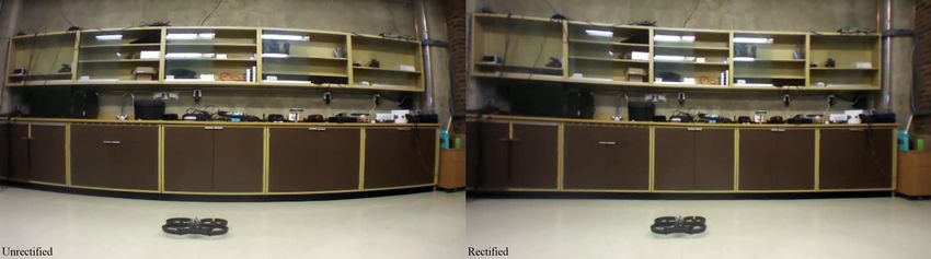
Eight trials were conducted to collect data. A white curtain was used to provide a
best-case scenario for the object detection system. A complex background was also used to
provide more challenging conditions. Sample video frames from each type of background
are shown in Figures 6 and 7, respectively, with the raw (unrectified) view on the left and
the corrected (rectified) view on the right.
Figure 6. White curtain backdrop: unrectified (left), rectified (right).
Figure 7. Complex scene backdrop: unrectified (left), rectified (right).
The TensorFlow-based APIs were trained using unrectified images recorded from the
onboard camera. The Darknet-based YOLO v2 and Tiny YOLO were trained using both
unrectified (i.e., same as the TensorFlow-based APIs) and rectified images to provide more
comparisons in experimental testing and assess the importance of camera calibration for
the performance of the detection system. Note the target UAV ranging calculations were
performed under the standing assumptions listed in Section 2.4.
A sequence of flight experiments was performed. First, two trials of simple movements
in the side and height directions were performed, since these movements can be directly
measured from the onboard camera view. Next, two trials of back and forth movements in
the depth direction were run. These are more challenging since the depth estimation relies
entirely on the quality of the estimated bounding box, as shown in Section 2.4. Following
this, two trials of UAV rotations were conducted. Due to the shape of the drone, rotation
of the vehicle about the vertical axis causes the bounding box to change size. These two
trials are thus intended to test the robustness of detection when the target changes yaw
angle. Finally, two trials of complex flight patterns were conducted. These two operations
are intended to replicate realistic flight scenarios.Drones 2021, 5, 37 15 of 26
4.2.1. Offset in Vicon Camera System
Within the Vicon motion-capture system, each of the two UAVs is modeled as a rigid
body with a body-fixed frame at its geometric center, as illustrated in Figure 8. Relative
distances are measured from the center of one rigid body representing a UAV to the center
of the other one as shown in Figure 8.
Figure 8. Body-fixed frames defined within the Vicon motion capture system.
The relative distance calculations from Section 2.4 based on the estimated bounding
box actually provide the distance from the center of the lens of the pursuer UAV’s camera
to the center of the rear surface of the target UAV. As shown in Figure 9, the relative side
and height between the pursuer and target UAV is identical between the Vicon-based
measurements and the camera-based estimates, but the relative depth between the two
measurement methods will be different.
Figure 9. Relative depth estimation: Vicon versus camera-based calculations.
For consistency, all depth measurements will be reported in terms of the physical
offset, the distance from the pursuer UAV’s camera lens to the back surface of the target
UAV. The depth measurements obtained from the Vicon system are thus corrected as
DepthCamera = DepthVicon − OffsetDrones 2021, 5, 37 16 of 26
where the value of Offset was directly measured to be 44.4 cm.
4.2.2. Impact of Camera Calibration
Although the TensorFlow-based APIs were trained using a set of unrectified images,
the object detection system can detect the UAV in both rectified and unrectified camera
video feeds. The percentage differences between detection results in rectified and unrecti-
fied videos are shown in Table 5. Positive percentages indicate that more error is present in
rectified videos.
Table 5. Difference of TensorFlow Detection Results on Rectified and Unrectified Videos.
API x (%) y (%) z (%) Avg. (%)
SSD MobileNet v1 6.21 18.42 72.11 36.30
SSD Inception v2 3.85 25.74 73.59 35.70
Faster RCNN Inception v2 127 14.95 56.08 68.24
Table 5 shows that all of the APIs performed worse on rectified videos. This is a direct
result of training using only unrectified images. Faster RCNN Inception v2 has the most
difference in the detection results.
Darknet-based APIs were trained using both rectified and unrectified images. The
difference in detection performance between permutations of Rectified (R) and Unrectified
(U) images used for Training (T) and onboard Video (V) are shown in Table 6 for YOLO v2.
A positive percentage difference indicates the second setup has more error. For instance,
employing unrectified training and unrectified detection images gives better results than
unrectified training images and rectified detection images.
Table 6. Difference of YOLO v2 Performance for Rectified (R) and Unrectified (U) images in Training
(T) and Video (V).
Setup x (%) y (%) z (%) Avg. (%)
UT/UV vs. UT/RV 3.92 18.83 40.45 24.8
RT/ UV vs. RT/RV 16.51 28.68 4.61 15.09
UT/UV vs. RT/RV −1.90 18.05 3.06 6.40
Table 6 shows that detection results are better with the UT/UV setup, which is
as expected since the object detection system is more familiar with unrectified images.
Similarly, RT/RV provides better results than RT/UV, due to the mismatch in the latter.
The RT/RV is actually slightly worse than UT/UV, which indicates the camera rectification
process is introducing errors into the detection results. This may be due to inaccuracies
in the camera K and/or projection P matrices of the camera, as covered in Section 2.5, in
which case the calibration should be redone. This issue may be aggravated by the relatively
low resolution of the onboard camera video feed (640 × 360), which causes the system to
be very sensitive to small imperfections in the rectification parameters.
Unlike YOLO v2, Tiny YOLO is unable to detect the drone when trained with an
unrectified training dataset. For a rectified training dataset, Tiny YOLO is able to detect the
target UAV in both rectified and unrectified camera videos. When compared to detection
on unrectified videos, detection on rectified videos is 5.01% worse along the side x axis,
9.66 % worse along the height y axis, and 1.5% better along the depth z axis. The average
of the distance estimations along the x, y, and z axes are 1.53% worse with RV than with
UV. The reasons are likely the same as those given in the previous paragraph.
4.2.3. Accuracy of Object Detection Systems
We will now compare the accuracies of the different object detection systems. Since all
the tested object detection systems were trained with the same set of unrectified images,Drones 2021, 5, 37 17 of 26
we will use the unrectified training/unrectified video setup to compare the accuracies of
SSD MobileNet v1, SSD Inception v2, Faster RCNN Inception v2, and YOLO v2. Tiny
YOLO does not detect anything with the UT/UV setup, thus YOLO v2 and Tiny YOLO are
compared using the RT/RV setup.
The first set of flights involve the target drone moving in the side and height directions.
The RMS errors along the x, y, and z directions are given in the tables below. Tables 7 and 8
provide the RMS errors when the flights are conducted in front of a white background,
while Tables 9 and 10 list the RMS errors for flights over a complex background.
Table 7. RMS Errors for side and height flights over white background, UT/UV setup.
Detection System x (cm) y (cm) z (cm) Avg. (cm)
SSD MobileNet v1 12.08 9.84 37.21 19.71
SSD Inception v2 11.43 8.00 23.57 14.33
Faster RCNN Inception v2 11.33 7.76 19.96 13.02
YOLO v2 12.37 6.48 19.35 12.73
Table 7 shows that Faster RCNN Inception v2 has the lowest error in the x direction
while YOLO v2 has the lowest error in the y and z directions. YOLO v2 has the lowest
average error, making it the most accurate in these test flights.
Table 8. RMS Errors for side and height flights over white background, RT/RV setup.
Detection System x (cm) y (cm) z (cm) Avg. (cm)
YOLO v2 11.84 7.06 20.82 13.24
Tiny YOLO 13.18 5.64 32.19 17.00
Table 8 shows that Tiny YOLO has a larger side and depth error but a smaller height
error than YOLO v2. Overall, YOLO v2 has a smaller average RMSE.
Table 9. RMS Errors for side and height flights over complex background, UT/UV setup.
Detection System x (cm) y (cm) z (cm) Avg. (cm)
SSD MobileNet v1 11.69 15.93 18.88 15.50
SSD Inception v2 10.62 14.70 8.58 11.30
Faster RCNN Inception v2 16.81 9.14 32.41 19.45
YOLO v2 15.01 11.39 40.19 22.20
Table 10. RMS Errors for side and height flights over complex background, RT/RV setup.
Detection System x (cm) y (cm) z (cm) Avg. (cm)
YOLO v2 47.72 19.82 37.53 35.02
Tiny YOLO 14.96 10.15 44.15 23.09
Tables 9 and 10 show that SSD MobileNet v1 and SSD Inception v2 have lower
RMS errors than Faster RCNN Inception v2 and YOLO v2, particularly along the depth
direction. Tiny YOLO outperforms YOLO v2 along the side and height directions but not
the depth direction.
The next set of experiments involves the target drone flying along the depth (z)
direction over both a white and complex background. This flight pattern is used to test the
accuracy of the distance estimation. Unlike the previous set of flights, the bounding box
size changes substantially during these experiments. The resulting RMS errors are listed in
Tables 11 and 12 for the white background and Tables 13 and 14 for a complex background.Drones 2021, 5, 37 18 of 26
Table 11. RMS Errors for depth flights over white background, UT/UV setup.
Detection System x (cm) y (cm) z (cm) Avg. (cm)
SSD MobileNet v1 12.86 6.86 30.44 16.72
SSD Inception v2 12.52 4.78 21.02 12.77
Faster RCNN Inception v2 11.61 5.42 17.23 11.42
YOLO v2 12.45 4.28 17.25 11.33
Table 12. RMS Errors for depth flights over white background, RT/RV setup.
Detection System x (cm) y (cm) z (cm) Avg. (cm)
YOLO v2 12.04 4.95 18.89 11.96
Tiny YOLO 11.80 3.75 20.27 11.94
Tables 11 and 12 show that when testing over a white background, YOLO v2 has
equal or better accuracy than the TensorFlow-based systems and approximately equal
performance to TinyYOLO.
Table 13. RMS Errors for depth flights over complex background, UT/UV setup.
Detection System x (cm) y (cm) z (cm) Avg. (cm)
SSD MobileNet v1 7.65 16.18 22.70 15.51
SSD Inception v2 7.50 13.10 17.15 12.58
Faster RCNN Inception v2 11.33 7.21 25.69 14.75
YOLO v2 15.17 10.20 37.67 21.01
Table 14. RMS Errors for depth flights over complex background, RT/RV setup.
Detection System x (cm) y (cm) z (cm) Avg. (cm)
YOLO v2 39.73 24.05 41.10 34.96
Tiny YOLO 15.04 12.23 59.65 29.98
Table 13 shows that for a complex background, the TensorFlow-based detection
systems outperform YOLO v2 along the side x and depth z directions, with a pronounced
difference for the latter. SSD Inception v2 has the least RMS error along all three axes.
Meanwhile Table 14 shows that Tiny YOLO greatly outperforms YOLO v2 along the side
and height directions, while YOLO v2 outperforms Tiny YOLO along the depth direction.
This same trend was previously observed in Table 10 for side and height flight patterns.
The next flight involves the target UAV performing 360◦ rotations about its vertical
axis, in order to investigate the impact of changing the viewing angle on distance estimation
(as discussed in Section 2.4). The corresponding RMSE results for the different object
detection systems are given in Tables 15–18.
Table 15. RMS Errors for rotation flights over white background, UT/UV setup.
Detection System x (cm) y (cm) z (cm) Avg. (cm)
SSD MobileNet v1 16.38 7.02 31.43 18.28
SSD Inception v2 16.49 5.21 20.28 14.00
Faster RCNN Inception v2 15.31 4.92 19.13 13.12
YOLO v2 15.57 4.31 18.87 12.92Drones 2021, 5, 37 19 of 26
Table 16. RMS Errors for rotation flights over white background, RT/RV setup.
Detection System x (cm) y (cm) z (cm) Avg. (cm)
YOLO v2 15.88 4.70 16.91 12.50
Tiny YOLO 17.15 4.08 26.44 15.89
Table 15 shows that over a white background, SSD MobileNet v1 performs worse
than SSD Inception v2, Faster RCNN Inception v2, and YOLO v2, which in turn perform
similarly to each other, with YOLO v2 having the best performance by a small margin.
Table 16 shows that in these conditions, YOLO v2 greatly outperforms Tiny YOLO in depth
estimation, while being slightly better along the side x and slightly worse along the height
y direction.
Table 17. RMS Errors for rotation flights over complex background, UT/UV setup.
Detection System x (cm) y (cm) z (cm) Avg. (cm)
SSD MobileNet v1 14.62 14.96 15.22 14.93
SSD Inception v2 13.70 11.96 19.45 15.04
Faster RCNN Inception v2 18.90 7.01 33.84 19.91
YOLO v2 20.84 9.35 37.28 22.49
Table 18. RMS Errors for rotation flights over complex background, RT/RV setup.
Detection System x (cm) y (cm) z (cm) Avg. (cm)
YOLO v2 34.52 11.80 37.80 28.04
Tiny YOLO 20.74 9.20 39.02 22.99
When rotation flights are conducted over a complex background, Table 17 shows SSD
MobileNet v1 and SSD Inception v2 have similar performances to each other and have
clearly superior depth estimation as compared to Faster RCNN Inception v2 and YOLO v2,
which have similar performance levels. Table 18 shows Tiny YOLO has a strong advantage
over YOLO v2 along the side axis, a small advantage along the vertical axis and small
disadvantage along the depth axis.
The final set of flight tests involves trajectories consisting of translations along all
three axes as well as rotations. The resulting RMS errors are listed in Tables 19–22.
Table 19. RMS Errors for trajectory flights over white background, UT/UV setup.
Detection System x (cm) y (cm) z (cm) Avg. (cm)
SSD MobileNet v1 14.69 5.67 28.91 16.42
SSD Inception v2 13.78 5.12 21.68 13.53
Faster RCNN Inception v2 13.76 5.94 18.35 12.68
YOLO v2 14.79 3.92 15.00 11.24
Table 20. RMS Errors for trajectory flights over white background, RT/RV setup.
Detection System x (cm) y (cm) z (cm) Avg. (cm)
YOLO v2 14.46 5.43 14.96 11.62
Tiny YOLO 14.74 3.42 19.32 12.49
For trajectory flights over a white background, Tables 19 and 20 show that YOLO
v2 has the best average performance over both the TensorFlow-based SSD MobileNet v1,
SSD Inception v2 and Faster RCNN Inception v2, and the DarkNet-based Tiny YOLO. In
particular, the depth estimation for YOLO v2 is noticeably better than for the other object
detection systems.Drones 2021, 5, 37 20 of 26
Table 21. RMS Errors for trajectory flights over complex background, UT/UV setup.
Detection System x (cm) y (cm) z (cm) Avg. (cm)
SSD MobileNet v1 13.62 16.51 18.92 16.35
SSD Inception v2 13.18 19.17 30.49 20.95
Faster RCNN Inception v2 17.68 7.75 34.25 19.89
YOLO v2 15.89 7.06 52.38 25.11
Table 22. RMS Errors for trajectory flights over complex background, RT/RV setup.
Detection System x (cm) y (cm) z (cm) Avg. (cm)
YOLO v2 44.59 29.99 44.68 39.75
Tiny YOLO 17.42 10.42 50.31 26.05
Conversely, when flying over a complex background, Table 21 shows that YOLO
v2 has a much larger depth estimation error than the TensorFlow-based object detection
systems. However, it has middle of the pack performance along the side (x) direction
and the best performance along the vertical (y) direction. Table 22 shows that YOLO v2
outperforms Tiny YOLO for depth estimation but is much worse along the remaining x
and y directions.
To summarize the previous results, all five object detection systems are capable of
finding the target UAV whether it is flying over a simple (white curtain) background or a
complex one. In all tests, estimation along the depth (z) direction has a larger error than es-
timation along the side (x) and height (y) directions. This is due to a combination of factors,
including errors in the camera calibration (c.f. Section 4.2.2) as well as imperfect detected
bounding boxes (IoU < 1, c.f. Section 2.3). Tables 23 and 24 show the average of the RMS
errors attained in the various flight tests (side and height, depth, rotation and trajectory)
for each of the object detection systems over both a white and complex background.
Table 23. Average of RMS Errors for Flights, UT/UV Setup.
Detection System Simple BG Complex BG
RMSE Avg. (cm) RMSE Avg. (cm)
SSD MobileNet v1 17.78 15.57
SSD Inception v2 13.66 14.97
Faster RCNN Inception v2 12.56 18.50
YOLO v2 12.50 22.70
Table 24. Average of RMS Errors for Flights, RT/RV Setup.
Detection System Simple BG Complex BG
RMSE Avg. (cm) RMSE Avg. (cm)
YOLO v2 12.33 34.44
Tiny YOLO 14.33 25.27
Table 23 shows that over a white background, YOLO v2 performs the best, followed
closely by Faster RCNN Inception v2. Conversely, over a complex background, YOLO v2
and Faster RCNN Inception v2 are the lowest and second-lowest performers, respectively.
Meanwhile, Table 23, which compares only the Darknet-based YOLO v2 and Tiny YOLO
using the rectified training/rectified video setup shows that YOLO v2 performs better than
Tiny YOLO over a white background, yet substantially worse over a complex background.
A consistent trend which can be observed throughout all the flight testing in this
section is that for the Darknet-based object detection systems YOLO v2 and Tiny YOLO;
the accuracy becomes substantially worse when the UAV is flown over a complex (realistic)
background as opposed to a simple (plain white curtain) background. The reason forDrones 2021, 5, 37 21 of 26
this is that the accuracy of the estimated bounding boxes by both these systems exhibits
significant levels of misdetections and outliers in the complex background setup. Figure 10
visually illustrates a best-case scenario, where the bounding boxes are both accurate and
tight around the target UAV. Figures 11 and 12 visually illustrate two failure modes,
loose bounding boxes and wrong bounding boxes respectively, both of which skew the
target position estimation and thus increase the overall RMS error. While these failure
modes are inevitable for all object detection systems, we see that the TensorFlow-based
SSD MobileNet v1, SSD Inception v2, and Faster RCNN Inception v2 have more robust
detection performance, meaning their RMSE numbers are closer to each other between the
simple and complex background cases.
Figure 10. Examples of Accurate Bounding Box.
Figure 11. Examples of Loose Bounding Box.
Figure 12. Examples of Wrong Bounding Box.
4.3. Consistency Results Discussion
For the third and final evaluation of the object detection systems, we compute their
experimental consistency in terms of the mean Average Precision (mAP) metric introduced
in Section 2.3. The IoU threshold settings for all of the detection systems was set to 0.5. This
is already the default threshold for the TensorFlow-based SSD MobileNet v1, SSD Inception
v2, and Faster RCNN v2. The default IoU thresholds of YOLO v2 and Tiny YOLO are 0.2,
and so these were adjusted to 0.5 for fairness of comparison.
The mAP for the flight tests along the side and height directions are given in
Tables 25 and 26 for the unrectified training/unrectified video setup (used by the
TensorFlow-based object detection systems plus YOLO v2) and rectified training/rectified
video setup (used by the Darknet-based YOLO v2 and Tiny YOLO), respectively.Drones 2021, 5, 37 22 of 26
Table 25. mAP for Side and Height flights, UT/UV Setup.
Object Detection System Simple BG Complex BG
SSD MobileNet v1 0.8442 0.8226
SSD Inception v2 0.8045 0.7259
Faster RCNN Inception v2 1.0000 0.9555
YOLO v2 1.0000 0.5151
Table 26. mAP for Side and Height flights, RT/RV Setup.
Object Detection System Simple BG Complex BG
YOLO v2 1.0000 0.9525
Tiny YOLO 0.5559 0.7097
The mAP for the flight tests along the depth axis are given in Tables 27 and 28.
Table 27. mAP for Depth flights, UT/UV Setup.
Object Detection System Simple BG Complex BG
SSD MobileNet v1 0.9277 0.6229
SSD Inception v2 0.6485 0.5726
Faster RCNN Inception v2 1.0000 0.9739
YOLO v2 0.9945 0.6578
Table 28. mAP for Depth flights, RT/RV Setup.
Object Detection System Simple BG Complex BG
YOLO v2 1.0000 0.9738
Tiny YOLO 0.3933 0.8603
The mAP for the flight tests involving rotations about the yaw axis are given in
Tables 29 and 30.
Table 29. mAP for Rotation flights, UT/UV Setup.
Object Detection System Simple BG Complex BG
SSD MobileNet v1 0.9130 0.9353
SSD Inception v2 0.8477 0.8160
Faster RCNN Inception v2 1.0000 0.9810
YOLO v2 1.0000 0.4610
Table 30. mAP for Rotation flights, RT/RV Setup.
Object Detection System Simple BG Complex BG
YOLO v2 1.0000 0.9726
Tiny YOLO 0.7626 0.8270
The mAP for the final set of tests involving flying a trajectory are given in
Tables 31 and 32.
Table 31. mAP for Trajectory flights, UT/UV Setup.
Object Detection System Simple BG Complex BG
SSD MobileNet v1 0.7921 0.8088
SSD Inception v2 0.9040 0.9137
Faster RCNN Inception v2 1.0000 0.9520
YOLO v2 0.9992 0.4643Drones 2021, 5, 37 23 of 26
Table 32. mAP for Trajectory flights, RT/RV Setup.
Object Detection System Simple BG Complex BG
YOLO v2 1.0000 0.9302
Tiny YOLO 0.7034 0.7274
The average of the mAP results from the four sets of flight tests are provided in
Tables 33 and 34.
Table 33. Average mAP, UT/UV Setup.
Object Detection System Simple BG Complex BG
SSD MobileNet v1 0.8693 0.7974
SSD Inception v2 0.8012 0.7571
Faster RCNN Inception v2 1.0000 0.9656
YOLO v2 0.9984 0.5246
Table 34. Average mAP, RT/RV Setup.
Object Detection System Simple BG Complex BG
YOLO v2 1.0000 0.9573
Tiny YOLO 0.6038 0.7811
From Table 33, we see that Faster RCNN Inception v2 has by far the best average
consistency, both over a white and a complex background. The other two TensorFlow-
based object detection systems, SSD MobileNet v1 and SSD Inception v2, both achieve
lower mAP scores than Faster RCNN Inception v2, but their performance is fairly even
between the white and complex background test environments. YOLO v2 is the most
uneven, showing near-perfect results over a white background and very weak results over
a complex background.
Comparing the two DarkNet-based object detection systems in Table 34, we see that
YOLO v2 greatly outperforms TinyYOLO. We also see that the reduction in mAP is much
less when moving from simple to complex background and actually increases in the case
of Tiny YOLO.
4.4. Choice of Object Detection System
After testing the different object detection systems for efficiency, accuracy, and con-
sistency, we will now assign an overall score to the performance of each object detection
system over a white and a complex background. Efficiency is assigned a relatively low
weight (20%) since it can be optimized by the implementation, for instance developing a
ROS package in C++ rather than Python to interface with the TensorFlow API. Accuracy
and consistency are both assigned a higher weight of 40% to recognize that they can be
improved by training the object detection system with more images but at the cost of a big
increase in required computational power for training, as well as the risk of overfitting.
Efficiency is scored based on running speed. The higher the frames per second (fps),
the better. We use only the run speed within ROS, since this is the environment used to
control the pursuer UAV, and assign the maximum possible score of 20 to 100 fps. The
resulting scores for both white and complex backgrounds are identical and are listed in
Tables 35 and 36 under the column “E”.
Accuracy is scored based on the average of the RMS error across all flight trials. The
lower the error, the better. In order to use the Unrectified Training/Unrectified Video
(UT/UV) framework for all five object detection systems, we use the ratio between YOLO
v2 and Tiny YOLO RMS errors under Rectified Training/Rectified Video (RT/RV) trials
listed in Table 24 to extrapolate the performance of Tiny YOLO in UT/UV. Referring to
Table 23 and defining that 0 cm RMSE scores 40 while 30 cm RMSE scores 0, the calculatedYou can also read