Experimental evaluation of the thermal conductivity for additive manufactured materials. New test facility concept and preliminary tests

Journal of Physics: Conference Series

PAPER • OPEN ACCESS

Experimental evaluation of the thermal conductivity for additive
manufactured materials. New test facility concept and preliminary tests
To cite this article: N Bianco et al 2021 J. Phys.: Conf. Ser. 1868 012008

View the article online for updates and enhancements.

 This content was downloaded from IP address 46.4.80.155 on 05/07/2021 at 21:46

2020 UIT Seminar on Heat Transfer (UIT-HTS 2020) IOP Publishing
Journal of Physics: Conference Series 1868 (2021) 012008 doi:10.1088/1742-6596/1868/1/012008

Experimental evaluation of the thermal conductivity for
additive manufactured materials. New test facility concept and
preliminary tests

 N Bianco1, R Mastrullo1, A W Mauro1 and L Viscito1*
 1
 Department of Industrial Engineering, Federico II University of Naples, P.le Tecchio
 80, 80125 Naples (Italy)
 *Corresponding author e-mail: luca.viscito@unina.it

 Abstract. Items for heat transfer made by metal foams or additive manufactured structures allow
 to create special components for several applications (i.e. fast response PCM, complex and light
 HEXs working at high temperatures for the aerospace sector). For their design thermo-physical
 properties data are required, such as thermal conductivity. To accurately measure this parameter
 with conventional procedures for metallic items (e.g. flash methods), the specific heat and
 density should be measured each time depending on the actual composition of the porous media
 (estimation is not yet reliable and porosity not known). The scope of this paper is to validate a
 test facility and the relative method for the data reduction to proof the possibility to measure
 directly the thermal conductivity with samples of small size. The experiments, carried-out with
 square samples (30x30 mm2), allow to measure a range of thermal conductivity between 5 and
 50 W/m K. The main aspect of the experimental method is the calibration of the heat losses
 towards the environment by means of a reverse technique. The assessment of the results against
 samples of known materials was good.

Keywords: thermal conductivity, test facility concept, additive manufacturing, UHTC materials

1. Introduction
In the last decades, it has become necessary to develop and produce geometrically complex items for
any kind of application. It is indeed important for the industrial sector to exploit new production
technologies aimed at the realization of innovative materials having more and more performing
mechanical and thermophysical properties. On this regard, the advent of 3-D printers has opened
complete new scenarios and great importance was attributed to the Additive Manufacturing (AM). This
technique largely differs from conventional items production processes, typically based on metals
melting or on chip-cutting machining that realize the desired object from a single block. The new AM
technique relies instead on a “layer-by-layer” procedure, consisting in the deposition of material in thin
layers, one above the others, in the form of metal wires, powders or liquids, catching the final CAD-
made 3-D sketch of the desired item. 3-D printing is already moving from a purely prototype technology
to an end-use manufacturing process. As a fact, the AM technique is becoming widely known since the
costs related to using 3-D printers have significantly decreased over the last years, allowing more and
more people and companies to have access to this technology [1]. Some examples can be given through
the exploitation of AM in creating replacement parts for old equipment, molds and tools able to assist
in manufacturing other products, and also the realization of brand new products that take advantage of
 Content from this work may be used under the terms of the Creative Commons Attribution 3.0 licence. Any further distribution
 of this work must maintain attribution to the author(s) and the title of the work, journal citation and DOI.
Published under licence by IOP Publishing Ltd 1

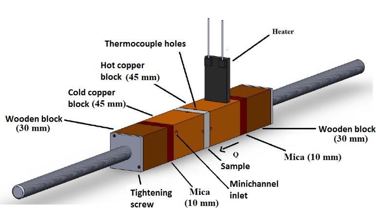
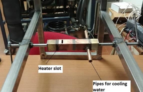
2020 UIT Seminar on Heat Transfer (UIT-HTS 2020) IOP Publishing
Journal of Physics: Conference Series 1868 (2021) 012008 doi:10.1088/1742-6596/1868/1/012008

the unique peculiarities allowed by AM. For instance, each layer can be made of a different material
thus having very heterogeneous combinations, with singular physical and mechanical characteristics,
exploitable in the biomedical field. Moreover, very complex geometries such as high efficiency heat
exchangers for aerospace applications can be easily realized by using AM [2], thus reducing weight and
limiting the number of individual components and connecting tools/bolts to assemble the final item.
 However, one major drawback of the AM technology is the complex determination of the material
properties [3], since the final product is neither homogeneous nor isotropic, but is rather considered an
anisotropic porous material with micro air bubbles randomly placed inside the object [4]. This
characteristic reflects on the evaluation of crucial thermophysical properties, such as the specific heat
and thermal conductivity, especially in case of heat exchangers or other thermal duty applications.
 The determination of the thermal conductivity is a key aspect also for other innovative materials,
such as Ultra-High Temperature Ceramics (UHTCs) employed in atmospheric entry operation of outer
space elements. The evaluation of the thermal conductivity for these porous materials at high
temperature is usually carried-out by employing difficult mathematical models [5], whereas on-field
tests are not performed due to the lack of a proper available method.
 Conventional available methods aimed at the evaluation of the thermal conductivity are unsuitable
for the abovementioned materials, and usually consist in steady state one dimensional experiments (“Hot
plate” procedure) or transient conduction tests (“Flash method”). In fact, the hot plate procedure
generally requires very large samples and is applied for light building insulating materials (thermal
conductivities less than 0.1 W/m K). The flash method is instead an indirect procedure and allows the
calculation of the thermal diffusivity, thus requiring the knowledge of the material density and specific
heat, usually unknown for heterogeneous and porous materials.
 For this reason, a heat conduction apparatus was specifically designed in this study to perform
experiments on materials in order to evaluate their thermal conductivity, within the range of 5-50 W/mK,
expected for AM and ceramic items, and temperatures up to 150 °C. The heat losses and the contact
thermal resistance of the samples were also characterized to enhance the accuracy of the results shown.
The set-up of the test facility was performed by using stainless steel (AISI-304L type), obtaining a good
agreement between experimental and provided thermal conductivity data.

2. Experimental facility

2.1. Test section and concept
The sketch and a photograph of the test facility is shown in Figure 1. The test rig concept is similar to
that conceived by Flaata et al. [6], proposing some modification related to the heating method and the
geometrical arrangement. It consists of a copper hot plate and a cold copper plate (390 W/m K) separated
by the specimen material, having a square cross section of 30x30 mm2. The heat is provided by Joule
effect thanks to a ceramic heater (Bach RC GmbH, customized), which is placed in a dedicated slot
carved in the hot copper block. The variable power supply is given by a DC power unit with a capacity
of 0-10 A and 0-40 V, by controlling the voltage value. A water multi-minichannel heat sink is obtained
at the edge of the cold copper block to cool down the test section. Both cold and hot blocks are then
connected to a mica block material (0.72 W/mK), a wood square block and a screwing system able to
tighten the whole structure. In order to avoid undesired relative rotations, two copper linchpins (1.5 mm
deep) are provided for each side of the specimen as connecting elements between the sample and the
copper blocks. The negligible alteration of the 1-D temperature field was verified with previous
simulations. Both copper blocks and the tested specimens were accurately polished before the set-up
operations, in order to obtain the best possible adherence between the surfaces. Moreover, a thermal
compound (3.2 W/mK) was placed among connecting parts as a further way to improve thermal contact.
Finally, four holes (diameter of 1.5 mm and 10 mm depth) are provided in the copper blocks right before
and after (less than 1.0 mm) the specimen, to allow the sample temperature measurements. In order to
ensure a fair estimation of the blocks temperature, all the 8 thermocouples were fastened with
cyanoacrylate glue inside their slots, in which a conspicuous amount of thermal compound was also
used. Other 2 T-type thermocouples are respectively placed close to the ceramic heater slot and in the
environment in order to estimate the maximum temperature reached in the test facility and the ambient

 2

2020 UIT Seminar on Heat Transfer (UIT-HTS 2020) IOP Publishing
Journal of Physics: Conference Series 1868 (2021) 012008 doi:10.1088/1742-6596/1868/1/012008

temperature during experiments, thus allowing the evaluation of the heating losses. The whole test
facility, horizontally arranged, was insulated with a considerable amount of synthetic foam (multiple
layers for a total amount of more than 15 cm) having a thermal conductivity lower than 0.07 W/m K, to
limit the heat losses to the surrounding ambient as much as possible and to corroborate the hypothesis
of one dimensional heat transfer in the test section. From a preliminary analysis performed with a
computational software, the hot copper block length was found to be largely sufficient to guarantee the
heat flux uniformity, in the whole range of experimented operating conditions.

 (a) (b)

Figure 1. (a) Schematic lay-out of the test rig with all the parts exposed; (b) Photograph of the test
section.

2.2. Measurement instrumentation
The temperature measurement at the specimen hot and cold edges is carried out by using eight T-type
thermocouples, respectively at the top, bottom, left and right sides for each copper block, very close to
the specimen section. Two additional T-type thermocouples are respectively located in the environment
and close to the heating section in the hot copper block. All the thermocouples signals are read by an
input voltage module that provides the desired temperature value with an overall accuracy of ±0.37 °C.
The DC power supply unit gives variable voltages and currents in the range of 0-40 V and 0-10 A,
respectively. The current is directly measured by the power supply unit, with an overall accuracy of
±0.2% of the reading, as stated by the manufacturer. The voltage applied to the ceramic heater is instead
measured with two wires directly applied on the heater nickel terminals, in order to compensate possible
voltage drops in the connecting copper wires. The voltage input module provides the measurement with
an overall accuracy of ±0.52%.

3. Method

3.1. Model and measurement algorithm
A linear function of the mean temperature value reached by the specimen during the experiment is
considered for the evaluation of the thermal conductivity, as shown in Equation (1):

 ̅ = + ∙ ̅ (1)

 The constants a and b are unknown and are calibrated according to a numerical model that follows
an iterative procedure, which will be shown in this section. According to Figure (2), is the sample
thickness, whereas ̅ and ̅ represent the mean measured temperature values of the four type-T
thermocouples placed before and after the sample, respectively. The thermal resistance of the copper
layers between the thermocouples location and the specimen surface has been neglected thanks to the
reduced distance and the very high thermal conductivity of pure copper (398 W/m K). The effective
heat load crossing the specimen is the measured electric power (equal to the product between the
imposed voltage and current) minus the heat losses in the hottest section close to the heater ( ,ℎ )

 3

2020 UIT Seminar on Heat Transfer (UIT-HTS 2020) IOP Publishing
Journal of Physics: Conference Series 1868 (2021) 012008 doi:10.1088/1742-6596/1868/1/012008

and the heat losses along the specimen extension ( , ). In this model, both hot and cold sides contact
resistances, named and , respectively, between the specimen and copper surfaces, are also taken
into account.

 Figure 2. Model concept

 The expression of the heater losses is presented in Equation (2), in which ℎ is the upstream
area of the sample, is the maximum measured temperature value reached during the tests from the
thermocouple placed close to the heater slot and represents the ambient temperature value:

 ,ℎ = ∙ ℎ ∙ ( − ) (2)

 Therefore, the current heat load right before the beginning of the sample is represented by the
difference between the electric power supplied to the specimen and the heater losses, in which 
coordinate is perpendicular to the specimen surface:

 = ( = 0) = − ,ℎ (3)

 The specimen temperature value for each z-axis position is given by an energy balance on the
specimen part of thickness dz:

 ( ) 
 ( ) = ( − ) − ∙(̅ ) (4)
 
 The specimen cross sectional area A is obtained by multiplying the exact measured values of two
sides L1xL2. For first and last elements of integration, Equation (4) also takes into account the hot 
and cold side contact resistances between the specimen and the copper surfaces. The local heat power
crossing the sample is obtained by Equation (5), where the subtractive term refers to the specimen losses,
which are a function of the local sample temperature and the ambient temperature.
 
 ( ) = − ∫0 ∙ 2 ∙ ( 1 + 2) ∙ ( ( ) − ) ∙ (5)

 The parameters , , , and are unknown, so their calibration is needed. An algorithm is
implemented and solved with a MATLAB code [7] and the following steps are executed:
 a) A triplet (i) of the values , and is fixed;
 b) The specimen thickness (j) is fixed among the available ones;
 c) The values of and are chosen (k);

 4

2020 UIT Seminar on Heat Transfer (UIT-HTS 2020) IOP Publishing
Journal of Physics: Conference Series 1868 (2021) 012008 doi:10.1088/1742-6596/1868/1/012008

 d) The cold mean temperature of the model ( ̅ ) is calculated according to the numeric integration
 of Equation (4);
 e) For the whole set of N experiments at thickness (j), the error between the cold mean temperature
 of the model and the cold mean temperature measured by the thermocouples is evaluated,
 through the ( , , ) parameter, as shown in Equation (6):
 2
 ∑ ̅ ̅
 =1( − , ( , , ))
 ( , , ) = √ 
 (6)
 f) The procedure from point c) to e) is repeated for each values of and : in this way is it
 possible to estimate the minimum value of the error at each specimen thickness:
 ( , ) = min ( ( , , )) (7)
 g) This procedure is repeated for any specimen thickness (j) and for each triplet (i), obtaining an
 array of the error sums:
 _ ( ) = ( ( , )) (8)
 h) The minimum value of the array determines the triplet values of the parameters , and ,
 from which the and values are finally obtained for each sample thickness.

3.2. Uncertainty analysis
The uncertainty of the measured parameters of interest was calculated by composing the instrumental
accuracy to the unavoidable fluctuations observed during the experiments, corresponding to the standard
deviation in the recording period. For the sample dimensions, a Vernier electronic caliper (±0.01 mm)
was employed with numerous (more than 30) measurements, with the results shown in Figure 3 of
paragraph 4.1. In case of derived parameters, the uncertainty was computed according to the law of
propagation of errors [8]. Either case, the expanded uncertainty was finally obtained by using a coverage
factor of 2, thus guaranteeing a confidence level higher than 95%. A summary of the calculated
uncertainty for all the parameters of interest is given in Table 1.

 Table 1. Uncertainty of the parameters of interest

 Parameter Calculated uncertainty
 (coverage factor = 2)
 Specimen temperatures ±0.4 °C
 Specimen Δ = ̅ − ̅ ±0.6 °C
 Heat power ±5.9%
 Thermal conductivity ±12.1%

3.3. Experimental procedure
All the tests are carried-out in steady state conditions, with a recording time and frequency of 120 s and
1 Hz, respectively. The desired heat rate across the specimen section is set by changing the DC voltage
applied to the ceramic heater. A constant water flow is given for the cold copper block to set the sink
temperature value. Power and temperatures values are then constantly monitored and controlled via user
interface and the system is let to stabilize until steady state condition is reached. Particularly, the
recording time was allowed to start only when the fluctuations of the 8 acquisition period did not exceed
0.3 °C (which is lower than the uncertainty of the measurement itself). The ambient temperature
fluctuation was also controlled and limited to 0.5 °C to avoid excessive variation of the heat losses.

4. Experimental results

4.1. Samples
The purpose of these tests was to validate the model and the experimental procedure. For this reason,
all experiments were carried-out by using stainless-steel (AISI 304 L), having a reference thermal

 5

2020 UIT Seminar on Heat Transfer (UIT-HTS 2020) IOP Publishing
Journal of Physics: Conference Series 1868 (2021) 012008 doi:10.1088/1742-6596/1868/1/012008

conductivity at 20 °C of around 15 W/m K, falling within the possible range of additive manufactured
and ultra-high temperature ceramics materials. However, the real thermal conductivity may slightly
differ from one manufacturer to another caused by minor chemical differences in the tested samples,
and its value can be estimated as a function of the temperature from different reference studies according
to their measurement procedure. Graves et al. [9] at the Oak Ridge National Laboratory (ORNL)
obtained the following equation, in which the temperature must be inserted in [K]:

 = 7.9318 + 0.023051 ∙ − 6.4166 ∙ 10−6 ∙ 2 (9)

 Bogaard [10] and Chu and Ho [11] also measured the thermal conductivity of AISI 304 L in the
temperature range of 300-700 K. The fitting equation for Chu and Ho [11] results is given as follows:

 ℎ = 8.021 + 0.02715 ∙ − 1.418 ∙ 10−5 ∙ 2 (10)

 In the present experimental campaign, five square samples with a different thickness were cut from
the same AISI 304 L (30x30 mm2) square rod. A picture of the specimens used and their dimensions
(L1xL2xs) is provided in Figure 3 and Table 2.

 Sample Size (L1xL2xs) Uncertainty
 [mm] [mm]
 Sample 10 30.04x30.04x9.95 0.03x0.03x0.03
 Sample 14 30.01x29.98x13.90 0.04x0.02x0.05
 Sample 20 30.02x29.98x19.95 0.04x0.02x0.03
 Sample 28 29.98x29.97x28.07 0.05x0.03x0.08
 Sample 35 29.98x29.98x35.04 0.04x0.03x0.02
 Table 2. Specimens dimensions obtained with
 Figure 3. AISI 304 L specimens used
 multiple caliper measurements

4.2. Operating conditions and results
For each specimen, 10 tests were carried out, for a total amount of 50 experiments. It is worth noting
that the number of available equations is higher than the number of the unknown constants, thus leading
to an overconstrained system. Tests were performed by varying the supplied heat power and controlling
the temperature differences across the sample in the range 5-50 °C. Lower differences were avoided to
preserve the good accuracy of the experimental results, whereas higher differences were not taken into
account in order to keep the assumption of “local” thermal conductivity measurements. A summary of
the operating conditions is given in Table 3.

 Table 3. Operating conditions explored in the present experimental campaign

 Sample ̅ − 
 ̅ [°C] Heat load [W] [°C]
 Sample 10 5.9-64.6 19.4-55.6
 Sample 14 4.5-47.4 18.3-48.1
 Sample 20 5-50 °C 3.2-33.8 18.4-45.9
 Sample 28 2.3-24.6 18.0-43.8
 Sample 35 1.9-20.1 18.2-42.4

 A coarse preliminary analysis was performed to evaluate the order of magnitude of the five constants
to be calibrated. According to this study, the range of variation of the desired parameters was limited to
the values provided in Table 4, that shows also the iteration steps considered. According to the algorithm
procedure described in the previous section, the results minimizing the computational errors are
provided in Table 5.

 6

2020 UIT Seminar on Heat Transfer (UIT-HTS 2020) IOP Publishing
Journal of Physics: Conference Series 1868 (2021) 012008 doi:10.1088/1742-6596/1868/1/012008

 Table 4. Iteration range and step of the constants to be calibrated

 a [W/m K] b [W/m K2] [W/m2 K] , [m2 K/W]
 Iteration range 11-16 0.010-0.025 0.5-3 1e-6 – 4e-5
 Iteration step 0.1 0.001 0.1 1e-6

 Table 5. Model results and minimum RMSE values

 Sample a [W/m K] b [W/m K2] [W/m2 K] [m2 K/W] [m2 K/W] RMSE [°C]
 Sample 10 1.1e-5 3.3e-5 0.027
 Sample 14 3.9e-5 4.0e-5 0.098
 Sample 20 13.9 0.02 1 3.3e-5 2.0e-6 0.056
 Sample 28 1.0e-6 3.8e-5 0.048
 Sample 35 1.0e-6 1.3e-5 0.094

 Once Equation (1) has been calibrated, the thermal conductivity of the samples as a function of the
mean specimen temperature is shown in Figure 4, together with the total (heater and specimen) thermal
losses. The experimental thermal conductivities are also compared to the reference functions given in
Equations (9) and (10), providing a good agreement, with Equation (1) graphically included in both
methods. Details on the assessment are provided in Table 5. No significant discrepancies are found
between the different specimens analyzed. The total thermal losses, modeled as increasing functions of
the temperature difference with the environment, are restrained to very low values and barely reach 2
W only when significant heat loads (more than 60 W) are applied.

 (a) (b)

Figure 4. (a) Thermal conductivity of the AISI 304 L specimens as a function of their mean temperature;
(b) Total heat losses as a function of the average temperature difference between the hot block and the
ambient.

 Table 5. Main assessment parameters

 RMSEChu RMSEORNL RMSENew model Average k Maximum k
 [W/m K] [W/m K] [W/m K] uncertainty [%] uncertainty [%]
 0.314 0.303 0.082 3.90 12.10

5. Conclusions
A testing apparatus was designed and constructed for the evaluation of the thermal conductivity of
additive manufactured AM or ultra-high-temperature-ceramics UHTCs materials employed for the
atmospheric entry of space vehicles.

 7

2020 UIT Seminar on Heat Transfer (UIT-HTS 2020) IOP Publishing
Journal of Physics: Conference Series 1868 (2021) 012008 doi:10.1088/1742-6596/1868/1/012008

 The test facility allows the characterization of small size square (30x30 mm2) specimens, covering a
thermal conductivity measurement range between 5 and 50 W/m K. A dedicated model was developed
and calibrated by taking into account the thermal losses to the surrounding environment and the contact
thermal resistance between the specimens and the cold and hot sections of the test facility.
 Five stainless-steel AISI 304 L specimens having thicknesses from 10 to 35 mm were tested with
mean temperatures from 18.0 to 55.6 °C to validate the procedure and the performance of the apparatus.
The results provided the thermal conductivity as a linear function of the mean sample temperature,
according to the expression = 13.9 + 0.02 ∙ W/m K (with T in [°C]), which is in reasonably good
agreement with two reference functions available from open literature, within the operating conditions
tested.
 The thermal conductivity mean uncertainty goes from a maximum value of 12.1% for the lowest
mean temperature of 18.0 °C to a minimum of 2.4% for the highest mean temperature of 55.6 °C. The
overall calibrated thermal losses towards the ambient are estimated to be in any case lower than 2 W.
 The proposed method has the advantage to allow tests on small size specimens giving as a result the
k as a function of the mean temperature. This feature is interesting for R&D activities where tests on
several samples produced with different mixing and processing parameters for the 3D printing process
are needed. At the same time, it requires 50 measurements in different conditions and a lot of caution
for the setting to limit local thermal contact resistances. This procedure therefore requires expertise and
it is suggested only for research laboratory activities and not for in line checks of industrial processes.
 Future plans for this project include the measurement of the thermal conductivity for a wide range
commercially available UHTCs materials and 3-D printed metal items, to determine capabilities and
possible limitations of this concept.

Acknowledgments
Luca Viscito received a grant at Federico II University of Naples (Italy), Department of Industrial
Engineering. Funded by Ministero dell'Istruzione dell'Università e della Ricerca (MIUR), via the project
PON “AIM: Attraction and International Mobility” (CUP: E66C18001150001), which is gratefully
acknowledged.

References
[1] Buchanan C and Gardner L 2019 Engin. Struct. 180 332-348
[2] Saltzman D, Bichnevicius M, Lynch S, Simpson T, Reutzel E, Dickman C and Martukanitz R
 2018 Appl. Th. Eng. 138 254-263
[3] Hwang S, Reyes E, Moon K, Rumpf R and Kim N 2014 Electr. Mater. 44 771-772
[4] Danes F, Garnier B and Dupuis T 2003 Int. J. Thermoph. 24 772
[5] Maxwell J C 1904 Oxford: Oxford University Press 1
[6] Flaata T, Michna G and Letcher T 2017 ASME 2017 Summer HT Conference
[7] MATLAB 2019a Release, Mathworks
[8] Moffat R J 1982 Trans. ASME: J. Fl. Eng. 104 250-260
[9] Graves R S, Kollie T G, McElroy D L and Gilchrist K E 1991 Int. J. Thermoph. 12 409-415
[10] Bogaard R H 1985 Proc. 18th Int. Conf. Therm. Conduct., New York 175-185
[11] Chu T K and Ho C Y 1978 Proc. 15th Int. Conf. Therm. Conduct., New York 79-104

 8