Explainable Artificial Intelligence for Reinforcement Learning Agents
←
→
Page content transcription
If your browser does not render page correctly, please read the page content below
DEGREE PROJECT IN COMPUTER SCIENCE AND ENGINEERING,
SECOND CYCLE, 30 CREDITS
STOCKHOLM, SWEDEN 2021

Explainable Artificial Intelligence
for Reinforcement Learning Agents

LINUS NILSSON

KTH ROYAL INSTITUTE OF TECHNOLOGY
SCHOOL OF ELECTRICAL ENGINEERING AND COMPUTER SCIENCE

Explainable Artificial
Intelligence for
Reinforcement Learning
Agents

LINUS NILSSON

Master in Robotics & Systems Control
Date: April 30, 2021
Supervisor: Joel Brynielsson
Examiner: Hossein Azizpour
School of Electrical Engineering and Computer Science
Host company: Swedish Defence Research Agency
Swedish title: Förklarbar artificiell intelligens för
förstärkningsinlärningsagenter
iii

Abstract
Following the success that machine learning has enjoyed over the last decade,
reinforcement learning has become a prime research area for automation and
solving complex tasks. Ranging from playing video games at a professional
level to robots collaborating in picking goods in warehouses, the applications
of reinforcement learning are numerous. The systems are however, very com-
plex and the understanding of why the reinforcement learning agents solve
the tasks given to them in certain ways are still largely unknown to the hu-
man observer. This makes the actual use of the agents limited to non-critical
tasks and the information that could be learnt by them hidden. To this end, ex-
plainable artificial intelligence (XAI) has been a topic that has received more
attention in the last couple of years, in an attempt to be able to explain the
machine learning systems to the human operators. In this thesis we propose
to use model-agnostic XAI techniques combined with clustering techniques
on simple Atari games, as well as proposing an automated evaluation for how
well the explanations explain the behavior of the agents. This in an effort to
uncover to what extent model-agnostic XAI can be used to gain insight into
the behavior of reinforcement learning agents. The tested methods were RISE,
t-SNE and Deletion. The methods were evaluated on several different agents
trained on playing the Atari-breakout game and the results show that they can
be used to explain the behavior of the agents on a local level (one individual
frame of a game sequence), global (behavior over the entire game sequence)
as well as uncovering different strategies used by the agents and as training
time differs between agents.
iv

Sammanfattning
Efter framgångarna inom maskininlärning de senaste årtiondet har förstärk-
ningsinlärning blivit ett primärt forskningsämne för att lösa komplexa uppgif-
ter och inom automation. Tillämpningarna är många, allt från att spela dator-
spel på en professionell nivå till robotar som samarbetar för att plocka varor
i ett lager. Dock så är systemen väldigt komplexa och förståelsen kring varför
en agent väljer att lösa en uppgift på ett specifikt sätt är okända för en mänsk-
lig observatör. Detta gör att de praktiska tillämpningarna av dessa agenter är
begränsade till icke-kritiska system och den information som kan användas för
att lära ut nya sätt att lösa olika uppgifter är dolda. Utifrån detta så har förklar-
bar artificiell intelligens (XAI) blivit ett område inom forskning som fått allt
mer uppmärksamhet de senaste åren. Detta för att kunna förklara maskininlär-
ningssystem för den mänskliga användaren. I denna examensrapport föreslår vi
att använda modelloberoende XAI tekniker kombinerat klustringstekniker på
enkla Atarispel, vi föreslår även ett sätt att automatisera hur man kan utvärdera
hur väl en förklaring förklarar beteendet hos agenterna. Detta i ett försök att
upptäcka till vilken grad modelloberoende XAI tekniker kan användas för att
förklara beteenden hos förstärkningsinlärningsagenter. De testade metoderna
var RISE, t-SNE och Deletion. Metoderna utvärderades på flera olika agenter,
tränade att spela Atari-breakout. Resultatet visar att de kan användas för att för-
klara beteendet hos agenterna på en lokal nivå (en individuell bild ur ett spel),
globalt beteende (över den totala spelsekvensen) samt även att metoderna kan
hitta olika strategier användna av de olika agenterna där mängden träning de
fått skiljer sig.
Contents
1 Introduction 1
1.1 Detailed Problem Description . . . . . . . . . . . . . . . . . 2
1.2 Outline . . . . . . . . . . . . . . . . . . . . . . . . . . . . . 3
2 Related Work 4
3 Theory 8
3.1 Reinforcement Learning . . . . . . . . . . . . . . . . . . . . 8
3.1.1 Deep Q-Network DQN . . . . . . . . . . . . . . . . . 9
3.1.2 DQN extensions: Double DQN and Dueling DQN . . 12
3.2 Explainable AI . . . . . . . . . . . . . . . . . . . . . . . . . 14
3.2.1 RISE . . . . . . . . . . . . . . . . . . . . . . . . . . 14
3.2.2 t-SNE . . . . . . . . . . . . . . . . . . . . . . . . . . 17
3.3 Evaluation Metrics . . . . . . . . . . . . . . . . . . . . . . . 19
3.3.1 Area Under Curve (AUC) . . . . . . . . . . . . . . . 19
3.3.2 Deletion . . . . . . . . . . . . . . . . . . . . . . . . . 19
4 Methodology 22
4.1 Intuition . . . . . . . . . . . . . . . . . . . . . . . . . . . . . 23
4.2 Training DQN Agents . . . . . . . . . . . . . . . . . . . . . . 24
4.2.1 Agent Configuration and Training Setup . . . . . . . . 24
4.3 RISE and Generating Heat Maps . . . . . . . . . . . . . . . . 26
4.3.1 Setting up RISE . . . . . . . . . . . . . . . . . . . . 26
4.3.2 Generating Heat Maps . . . . . . . . . . . . . . . . . 27
4.4 Evaluating Explanation Using Deletion . . . . . . . . . . . . 27
4.5 Clustering With t-SNE . . . . . . . . . . . . . . . . . . . . . 28
5 Results 29
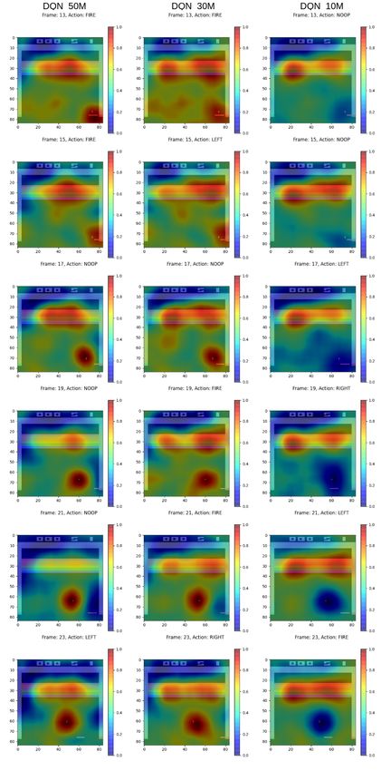
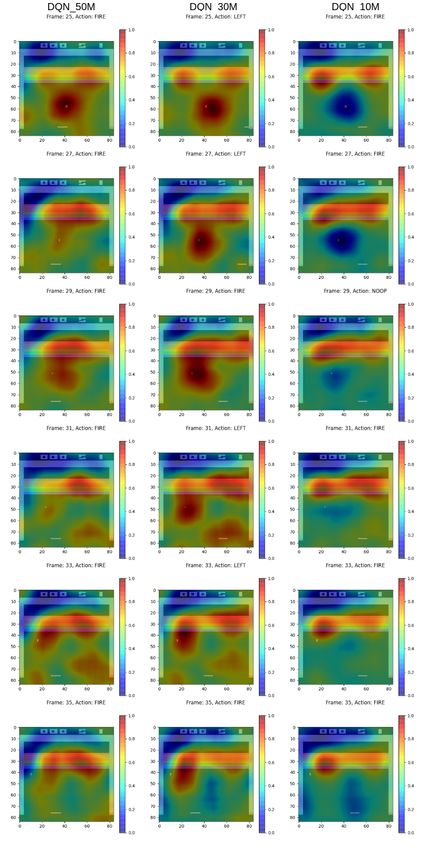
5.1 Generated Heat Maps . . . . . . . . . . . . . . . . . . . . . . 29
5.2 Results of Deletion Evaluation . . . . . . . . . . . . . . . . . 35
v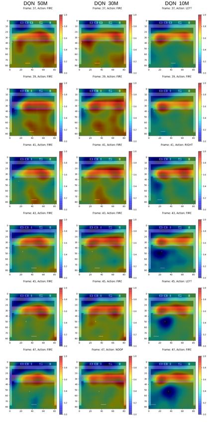
vi CONTENTS
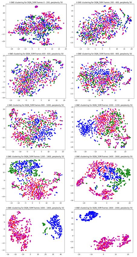
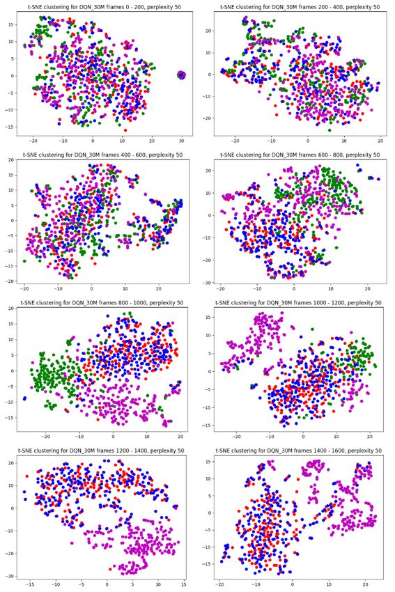
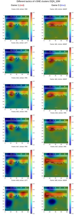
5.3 Results of t-SNE Clustering . . . . . . . . . . . . . . . . . . . 35
6 Discussion 43
6.1 The Importance of Explainability . . . . . . . . . . . . . . . . 43
6.2 Difficulties Using the Selected Methods . . . . . . . . . . . . 44
6.3 Understandability of Agent Behavior . . . . . . . . . . . . . . 45
6.4 Ethics and Sustainability . . . . . . . . . . . . . . . . . . . . 47
7 Conclusions 49
Bibliography 50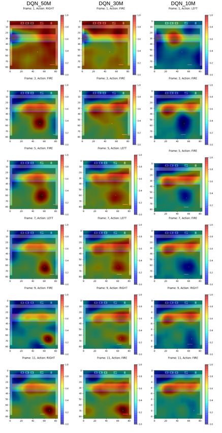
Chapter 1

Introduction

Since the early 2000s, machine learning (ML) has been steadily gathering
more interest from the public and the research community. In particular, neural
networks (NNs) have been used to solve a variety of different problems. NNs
have a desirable property of being universal function approximations. As such,
NNs have been successfully applied to a multitude of different tasks, ranging
from sentiment analysis of a text to large scale image classification [1, 2]. In
2012 Krizhevsky, Sutskever, and Hinton [3] applied convolutional neural net-
works (CNNs) to the ImageNet challenge, outperforming its peers. Since then,
CNNs have become a staple in the ML community.

Mnih et al. [4] brought the CNN architecture to the reinforcement learning
(RL) field when they proposed the deep Q-network algorithm, which uses
CNNs to approximate its reward function. It was impressive in that it could
learn to play a wide variety of Atari games without changing the network ar-
chitecture and the hyperparameters used. This was a major step forward as RL
algorithms up to this point had mostly been handcrafted and did not transfer
well to different types of problems. Since then RL has been applied to more
complex environments with impressive results. In several cases the trained
agents have exhibited near superhuman performance and showed interesting
behaviors out of the ordinary. Liu et al. [5] showed that agents trained to play
hide-and-seek could exploit objects in the environment to complete various
tasks, such as blocking entrance points to prevent the opposing team to find
their hiding spot, and managing to get on top of boxes and walk and thus make
the box move while the agent is still on top of it (something that is not readily
apparent as the boxes are, at first glance, meant to be pushed; hence, the agents
have successfully learnt a behavior allowing them to move the box by walking

                                       1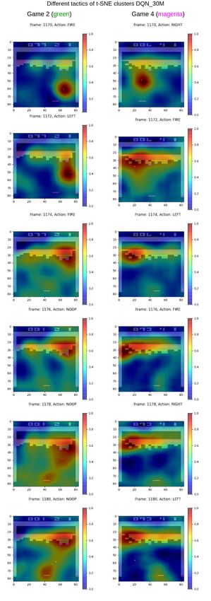
2     CHAPTER 1. INTRODUCTION

on top of it). This behavior of walking on top of boxes to move them, allowed
the agents to get over obstacles and walls placed by the opposing team. The
agents that were on the team tasked with hiding were also observed throwing
objects out of the playing field, so that the opponents could not use them in
their attempt to find their location. Silver et al. [6] trained an RL agent to play
the game Go and managed to beat the reigning human world champion dur-
ing several games with their AlphaGo algorithm. This accomplishment was
then followed up with AlphaZero [7] which managed to beat AlphaGo without
any input from humans within mere days of training. These types of accom-
plishments make RL an interesting field to study as they tend to exhibit clear
strategies and complex ways of solving tasks that are not obvious to humans.

The use of NNs is, however, a double-edged sword due to that the networks are
often very hard for humans to interpret. One can clearly observe the input to
the network and what the output is, but what actually matters for classification
or making decisions is obscured within a black box. This has major implica-
tions in that it lowers the trust in systems, and much of the information that
could be used to gain a deeper understanding of the problem is also hidden. To
combat this, a new field has emerged within ML, namely explainable artificial
intelligence, XAI. XAI tries to bridge the gap by providing explanations to the
decisions made by ML algorithms. Given the interesting strategies and behav-
iors that RL agents tend to exhibit, it would be interesting to learn more about
what makes the agent decide on certain strategies given a scenario. Similar to
other ML problems, this is hidden by the black box nature of the algorithms
used. There have been some research conducted related to XAI and RL [8, 9,
10], but the area is still in its infancy. There is much that could be gained by
being able to explain the agent behavior and strategy in a way that humans can
easily analyze. This project aims to investigate this further.

1.1      Detailed Problem Description
This project studied how existing XAI techniques can be combined and ap-
plied to RL agents to explain behaviors and strategies used by the agents. XAI
has been successfully employed in other machine learning fields, and has been
proven to provide valuable insights regarding the systems they are applied to.
Some work has been done to apply XAI to RL agents [10, 8, 9]. However,
much of the work use techniques that require access to the internals of the
model, introduce explainable training regimes, or instead use surrogate sys-
tems that are inherently more interpretable. This is limiting in the sense that
CHAPTER 1. INTRODUCTION               3

techniques that require access to the internals are often limited to a small set
of models to which they can be applied. Using techniques incorporated in
training excludes many current systems in use that one might wish to explain.
Employing a surrogate that replaces the actual system with a simpler model
might produce the same end results, but the reasoning of the system will then
vary from the reasoning that was to be explained.

The thesis project has been limited to only consider post-hoc techniques that
are applied after training has been done. A further requirement was that the
RL agents were considered to be black boxes, i.e., no access to the internals
of the system was given. Hence, only model-agnostic techniques were used
throughout the project, and the investigated XAI techniques should therefore
be possible to apply to any similar RL problem. This enables the techniques to
be used on models that have been trained with a variety of different algorithms
that are currently in use. The project also studied methods to automatically
evaluate how well explanations manage to capture the behavior and strategies
used by an RL agent. Hence, the aim of the project was to answer the following
research question:

   • To what extent can model-agnostic XAI techniques be used to gain in-
     sight regarding the behavior of RL agents?

1.2     Outline
The thesis follows the following structure. Chapter 2 presents related work
within the field of XAI and application of XAI on RL. Chapter 3 introduces
theory regarding the chosen XAI techniques, the theory needed to train the
RL agents, as well as techniques to evaluate explanations. Chapter 4 outlines
how the experiments were set up, what methods were chosen, and motivates
the research design. In Chapter 5 the results of the experiments in the form of
tables, graphs, and figures are presented. Chapter 6 disusses the results, and
how successful they were with regard to the research question. Lastly, Chap-
ter 7 presents the conclusions and provides some thoughts on further work that
ought to be done.
Chapter 2
Related Work
The XAI field of ML has been garnering more interest from the research com-
munity during the last couple of years. The increase in interest is mainly due
to the success that ML as a whole has enjoyed. This success has resulted in the
need to be able to better understand and analyze the models being used. Due
to the XAI field being a fairly recent research area there is a lack of consensus
on how the terminology within the field is being used. This lack of consen-
sus becomes apparent in that there is a mismatch between interpretability and
what this entails. An example of this is that in several works the key contribu-
tion related to explainability/interpretability is that one can replace a complex
model with a simpler representation, for instance a regression tree, as pre-
sented by Brown and Petrik [11]. This is an example of a common approach
where a surrogate using a simpler model is thought to be inherently more in-
terpretable to humans. However, it is debatable whether the surrogate system
actually explains the decisions made by the original network, as it is in fact
an entirely new system with its own set of properties that differ from the true
system. To get a good overview of the field and the terminology used within
XAI, the interested reader can find many examples of different methods in the
literature [12, 13, 14].
Given the recent success of using ML for image classification tasks, much
of the XAI focus has been on image classification systems. There exist several
methods that produce saliency maps as a means to explain the models used
for image classification. The intuition is that the saliency map highlights the
features of the input (i.e., the pixels in the image) that are of importance for the
system when making its decision about the image class. Some of the earliest
examples use gradients to compute saliency maps to highlight important fea-
4CHAPTER 2. RELATED WORK 5 tures in the input [15, 16, 17]. Similar to this, layer-wise relevance propagation (LRP) [18] instead looks at the relevance of each pixel in the input to highlight features of interest. DeepLIFT [19] is a method that produces saliency maps by comparing the activations of each neuron in the model layers. These tech- niques have all seen widespread use since their inception. They are, however, not model-agnostic since they require that the user has access to the model internals. Some are even limited to being applicable to a small set of model types with certain types of architectures. This poses issues due to the fact that it is not always the case that the end-user has access to the model internals or the necessary knowledge of the target system to be able to apply the XAI techniques. This can be both limiting and problematic. Systems that are al- ready in use might not allow accessing the internals, and there might have to be significant changes made to the architecture for the system to be compatible with the XAI technique in question. This would render any such technique to be ruled out. These techniques also limit the possibility to use the same ex- planation method for different types of model architectures. Having to use a specific XAI technique for each new model architecture is cumbersome, and might lead to them not being used at all. To come up with generic solutions, model-agnostic XAI techniques have been developed during the last couple of years. Examples of techniques that gar- nered much interest when they were published are RISE [20], LIME [21], and SHAP [22]. RISE is an XAI technique that produces heat maps for image classification problems. It does so by randomly masking the input image with a number of random masks. The masked inputs are then fed to the system, the probabilities are saved, and once all the masked inputs have been processed a heat map can be created consisting of the weighted average of all masks with their respective probabilities as weights. This technique is very simple to im- plement and can be used on any image classification system regardless of its architecture. Similar to this, LIME generates explanations by learning locally interpretable models around the outputs of any classifier. The local models are learned by sampling the vicinity of the input. The samples are then presented to the original network, and the outputs generated by the samples are used to construct the local model. LIME can be used to generate superpixel heat maps (the features of interest are highlighted using a so-called superpixel approach, where different superpixels capture different features), as well as some other types of explanations. In this sense, it is more versatile than RISE, but the heat maps generated by LIME are not as refined as those that RISE produces. This is due to the superpixel approach that LIME uses. SHAP is a widely used
6     CHAPTER 2. RELATED WORK

model-agnostic XAI technique. It is built on Shapley values [23] from game
theory. By using this approach the user can test the importance of different
features in the data in relation to the system which is being evaluated. SHAP
can be used on a wide variety of different types of problems, and is a strong
XAI technique in the sense that it is versatile. It can also be combined with
other XAI techniques to generate explanations, for instance, combined with
DeepLIFT [19] to create heat maps for deep neural networks. The explana-
tions provided by SHAP are, however, not as intuitive as those of LIME and
RISE, as they require that the end user has good knowledge of the target sys-
tems and the task at hand to fully understand them.

Combining model-agnostic and post-hoc XAI techniques and applying these
to RL problems, is something that has not been widely researched. Much of the
research instead focus on using techniques that require access to the internals
of the agents, use surrogates or depend on agents with explainability incorpo-
rated already at the training stage. Verma et al. [10] trained an RL agent with
a policy that focuses on using a high-level programming language as its input.
This is considered to be more interpretable as a human could understand the
policies by reading the programming language that is the output of their policy
network. InfoRL [24] uses information maximization to learn more ways of
completing a task in an RL setting. This, the authors mean, can be used to
provide a deeper understanding of why a certain course of action was chosen
by the agent. Yoon, Arik, and Pfister [25] use an RL setting to train a locally
interpretable model to a system. The model selects a small number of samples
and the training is then guided by a reward function as in a regular RL setting,
producing a locally interpretable model that can be used as a surrogate to the
black box system.

Mott et al. [9] presented an XAI technique specifically designed for explain-
ing RL agents. They achieve this by using an attention model and a top-down
approach that creates a bottleneck which forces the agent to focus on task-
relevant information in the state image. From this, attention maps of the state
image can be generated that point at what the agent focuses on during different
tasks. SpRAy [8] uses a similar approach to explain the behavior of RL agents
as the work conducted within the scope of this project. SpRAy implemented
a hybrid explanation technique using both LRP and the t-SNE [26] clustering
technique. LRP is applied to generate heat maps of what the agent finds im-
portant for each sample, and t-SNE is then used to cluster the heat maps in a
lower dimension based on similarities between heat maps in high-dimensional
CHAPTER 2. RELATED WORK                 7

space. This clustering allows the user to find similarities between heat maps
and can be used to find the behavior of the agent over time. The authors tested
their implementation on both image classification and on an RL agent trained
to play Atari-game [27] implementations. However, due to the use of LRP it
is not a model-agnostic approach (due to the fact that LRP requires access to
the internals of the system to be explained), but it is in essence very similar to
what this degree project aimed to achieve.

When applying SpRAy to an image classification algorithm it was found that
the algorithm classified images of horses solely by the presence of watermarks
in all the images containing horses. When instead applied to the RL agent
trained to play the game of Atari-Pinball it was found that the agent exploited
a bug within the environment that allowed the game to be tilted. These re-
sults point towards the need for any ML or RL system to be able to explain
themselves, as these exploits would otherwise have gone unnoticed, and the
systems would have failed on more challening problems.
Chapter 3

Theory

This chapter aims at giving an introduction to the theory of the methods im-
plemented for the degree project. The chapter is split into three sections, Sec-
tion 3.1 introduces reinforcement learning and policies used for training RL
agents. Section 3.2 introduces the XAI techniques used for explaining the RL
agents behavior. Lastly Section 3.3 introduces metrics for how the effective-
ness of explanations that the XAI techniques generate can be evaluated.

3.1      Reinforcement Learning
The RL problem consists of training an agent to perform various tasks within
an environment E by letting it interact with the environment and perform ac-
tions given by a policy approximated by a NN. The problem is particularly
hard given that the rewards rt , for a given action, are delayed in the sense that
an action at taken at the current time step might generate a reward several thou-
sand time steps later. The sparser these rewards are, the harder the problem
becomes. In contrast to supervised learning, the data is not labeled, and sam-
ples are dependent on one another. Executing an action at after seeing state
st at the current time step will determine the next state st+1 , that the agent
will see. So samples cant be assumed to be independent of one another. The
agent does not know at the current time which one of the valid actions that is
possible to take will generate a reward going forward, but must instead choose
an action depending on the current information with the goal of maximizing
rewards further ahead in time. The issue of rewards being delayed in time is
tackled by discounting rewards. In this approach an agent selects what action

                                        8
CHAPTER 3. THEORY 9
to take based upon maximizing the discounted sum of future rewards as:
T
0
X
Rt = γ t −t rt0 (3.1)
t0 =t
Where γ ∈ [0, 1] is the discount factor, T is the last time stamp in the se-
quence. As γ → 1 we make the agent more farsighted, accounting more for
future rewards. Fig. 3.1 describes the RL process per time step.
Environment
Reward
Interpreter
Action
State Agent
Figure 3.1: Flow chart of a simple RL setting.
What action the agent takes is decided by a policy, π, that is set up by the
user and approximated by a NN. In the thesis we consider a RL setup where
the agent interacts with the environment E. The agent interacts through a se-
quence, st , of actions, rewards and observations. The observations, xt ∈ RD ,
are pixel frames of the current environment and for each time step the agent
decides on an action to take based on the current observation. For the agent
to be able to fully grasp motion and direction in any state, 4 pixel frames are
stacked and presented to the agent. The action is passed to the environment
which changes state and computes a reward rt for the current time step. The
next section describes the DQN policy chosen to train the agents used for eval-
uation within the thesis project.
3.1.1 Deep Q-Network DQN
Deep Q-Network (DQN) [4] extends on the Q-Network [28] algorithm. When
presented in 2013, it was impressive in that it could play various Atari games10 CHAPTER 3. THEORY
using the same network structure and the same types of hyperparameters for
various games. In the setting of this project a DQN agent interacts with an
environment E in discrete time steps. Where the environment E is a video feed
of an Atari game. At each time step the agent sees a state st of E consisting
of N pixel frames xt . Each state is then st = (xt−N , ..., xt ). From observing
a state at each discrete time step the agent chooses an action at from a set
of allowed actions. The action is then fed to the environment, which in turn
changes its internal states accordingly and produces a new set of states st+1 and
a reward rt . To optimize training and data efficiency, DQN uses experience
replay, Lin [29]. During training of the agent, experiences are stored in D =
(e1 , e2 , ..., et ), where et = (st , at , rt , st+1 ). Mini batches are then sampled
randomly from D allowing the agent to train from many more samples than just
the experience at the current time step. This breaks up the inherent correlation
that is present between consecutive samples and alleviates some problems of
the agent diverging or getting stuck at local minima. The agent chooses actions
according to a stochastic policy π, with the goal of maximizing the sum of
expected discounted rewards from Eq. 3.1. For an agent following a policy π
the value function of the state action pair (s, a) is defined as
Qπ (s, a) = E [Rt |st = s, at = a, π] . (3.2)
Where the state-action value function Qπ is referred to as the Q-function and
π is a policy distribution over actions. Intuitively, Eq. 3.2 is the expected
rewards by taking action at after observing state st . At each time step, the
maximal future rewards that can be obtained in any state by following any
strategy is the optimal Q-function, Q∗ (s, a), defined as
Q∗ (s, a) = max E [Rt |st = s, at = a, π] . (3.3)
π
The optimal Q-function follows the Bellman equation, that is if we knew all
possible actions a0 of the next state s0 the optimal Q∗ (s0 , a0 ) would then simply
be to choose the action a0 that maximizes
h i
Q∗ (s, a) = Es0 ∼E r + γ max 0
Q ∗
(s 0 0
, a ) |s, a . (3.4)
a
However, since not all actions a0 are known for all next states s0 , a function
approximator for Q(s, a; θ) ≈ Q∗ (s, a) is used. The DQN algorithm uses a
Neural Network (NN) as the function approximator, with θ as its parameters.
Training of the NN that approximates the Q-function is done iteratively by op-
timizing sequences of loss functions, Li (θi ) that changes for each new iteration
i as:
Li (θi ) = Es,a∼ρ(·) (yi − Q (s, a; θi ))2 .
(3.5)CHAPTER 3. THEORY 11
Here yi is the target for iteration i of the loop, defined as
h i
0 0
yi = Es0 ∼E r + γ max 0
Q (s , a ; θ i−1 ) |s, a . (3.6)
a
ρ(·) is a probability distribution over sequences and actions called the behavior
distribution. For each iteration of the loop, the parameters are fixed to that of
the previous iteration θi−1 during optimization. Differentiating the loss func-
tion w.r.t. the weights θi , the loss function can be optimized via gradient based
methods. The gradient of the loss function is then
∇θi Li (θi ) =
h i
0 0
Es,a∼ρ(·);s0 ∼E r + γ max
0
Q (s , a ; θi−1 ) − Q (s, a; θ i ) ∇θ i
Q (s, a; θi )
a
(3.7)
Behavior Distribution and Epsilon-Annealing
Some time must be spent on discussing the behavior distribution ρ(s, a) as it
is an important part of training an agent using DQN. The agent selects actions
as a = maxa Q(s, a; θ). If only following this greedy strategy the chances
are the agent will not be able to perform adequately. If one considers the start
of a game this becomes apparent, the agent has not yet been presented with
many situations, so when deciding upon what action to take from maximizing
the future rewards will be based on a very small amount of experience. Thus,
only picking the maximal choice will most likely lead to the agent repeating
the same action over and over and learning will be slow. The behavior distri-
bution ensures that some measure of exploration is carried out. In general one
sets a behavior distribution that follows the greedy strategy with probability
1 − and chooses a random action with probability . This way the agent is
forced to explore other actions than that which gives the highest expected re-
turns.
For the agents trained in this project a behavior distribution was set with epsilon-
annealing. With epsilon-annealing the probability, , of taking a random action
starts out as 1.0. It is then linearly decreased over a fixed amount of time steps
to some small final such as 0.01. This is sometimes called the exploration-
exploitation trade-off. Starting out, the agent has very little knowledge of the
environment, and should then explore as much as possible. After training for
some time while exploring, it should transition over to using its gained knowl-
edge and exploit this. Epsilon-annealing is well suited for this as it selects12 CHAPTER 3. THEORY
random actions with close to 100% probability starting out, then moves over
to selecting actions randomly with very low probability and the agent instead
plays by learned experience.
3.1.2 DQN extensions: Double DQN and Dueling DQN
The original DQN algorithm has some drawbacks, it is quite slow to train and
tend to overestimate action values due to estimation errors. 2 papers have ad-
dressed these issues. Double DQN [30] deals with the issue of overestimating
Q-values. Wang et al. [31] introduced Dueling Q-Network that outperforms
the original DQN models. Both of these advances can be incorporated into
the original DQN network structure.
Double DQN
The Bellman equation, Eq. 3.4, maximizes over the expected action values,
this maximization tends to prefer overestimated Q-values over underestimated
ones. If the estimations had been uniform in the sense that all values were over-
estimated the policy would still perform, since the relative preference between
actions would be preserved. However, since values can be both over and un-
derestimated, thus not being uniform, the relative preference is not preserved
and overestimated values tend to be preferred by the maximization step. The
Double DQN approach solves this by letting the main DQN network estimate
the action a0 in the next state s0 that maximizes arg maxa0 Q(s0 , a0 ; θi ), the tar-
get network then estimates the Q-value for this action. This implies a change
to the target equation, Eq. 3.6, that can now be defined as
DDQN 0 0 0 −
yi = r + γQ s , arg max 0
Q (s , a ; θi ) ; θ , (3.8)
a
where θ− is a separate set of weights for the target network. Following this the
loss function Li (θi ) in equation, Eq. 3.5, is updated accordingly
2
DDQN
Li (θi ) = Es,a∼ρ(·) yi − Q (s, a; θi ) . (3.9)
Due to noise in the target networks estimation the Q-values will on average
be lower and less confident, thus removing some of the issues arising from
overestimated Q-values.CHAPTER 3. THEORY 13
Dueling DQN
For many RL problems it is unnecessary to estimate the value of each possible
choice of action in each state. As an example, when playing Atari-Breakout,
when the ball is moving away from the paddle, it is makes no difference to
move left, right or to take no action at all, in contrast once the ball is travelling
towards the paddle it is of high importance to choose the correct action as to not
miss the ball and potentially lose the game. Dueling DQN [31] builds on this
idea by replacing the fully connected layer of the original DQN arcithecture
with 2 separate fully connected layers that each estimate separate quantities.
The difference between the Dueling DQN and DQN architectures is shown in
Fig. 3.2.
Figure 3.2: Overview of the network architectures for: (top) Dueling DQN
and (bottom) regular DQN.
The Q-function, Qπ (s, a) is now estimated by combining 2 separate streams14 CHAPTER 3. THEORY
of estimation functions, namely the value function, V π (s), defined as
V π (s) = Ea∼π(s) [Qπ (s, a)] (3.10)
and Aπ (s, a) called the advantage function, defined as
Aπ (s, a) = Qπ (s, a) − V π (s). (3.11)
Combining Eq. 3.10 and Eq. 3.11 give rise to a new formulation of the Q-
function that the NN estimates as
Q(s, a; θ, α, β) = V (s; θ, β)+
!
1 X (3.12)
A(s, a; θ, α) − A (s, a0 ; θ, α) ,
|A| a0
where β are the parameters of the fully connected layer estimating V π (s), α
the parameters of the fully connected layer estimating Aπ (s, a), θ the param-
eters of the convolutional layers and A is the action space. Intuitively the
dueling network can learn what states are useful without having to evaluate
every possible action in the state. One can think of the value function v(s) as
predicting the value of being in state s and the advantage function A(s, a) as
the advantage of performing action a in state s.
3.2 Explainable AI
This section introduces the theory for the main XAI techniques used in the
project. The techniques used were RISE [20] that generate heat maps for in-
put images by means of a weighted average over many randomly masked in-
puts. The second technique t-SNE [26] is a clustering technique that converts
high-dimensional data into matrices of pair-wise similarities and visualizes
the resulting similarities in a lower dimension space.
3.2.1 RISE
RISE [20] is a model-agnostic post-hoc XAI technique, it was developed for
deep learning networks that take images as input and output a probability dis-
tribution over the possible classes. RISE is essentially divided into three steps,
generating N random masks, applying the N random masks to copies of the
original input and feeding these to the model and computing the probabil-
ity distribution over classes. Lastly taking the sum of all masks, where eachCHAPTER 3. THEORY 15
mask is weighted by the probability of the class after the masked input was fed
through the model. A simple flow-chart of how the RISE algorithm operates
is given in Fig. 3.3.
Mask I M Class probs
NN f Heatmap
Weighted
sum
Figure 3.3: Scheme of RISE algorithm. I M indicates the element-wise
product between the original input image and the random mask carried out on
each color channel.
The steps of RISE are outlined in the following subsections.
Applying Random Masks
Let f : I → R be the black box model to be explained that takes as an input
a color image and outputs a probability distribution over the possible classes,
for a RL case the probability distribution over possible actions. Each input is
a color image, I, that is a mapping from pixel-coordinates to 3 color values,
such that each Λ = {1, ..., H}x{1, ..., W } is mapped to the 3 color values,
where Λ is the pixel space of size H × W . Let M : Λ → {0, 1} be a random
binary mask coming from the distribution D. The importance of each pixel
λ ∈ Λ is defined as the expected value over all possible masks given that pixel
λ is observed. That is:
SI,f (λ) = EM [f (I M )|M (λ) = 1] (3.13)16 CHAPTER 3. THEORY
Where f (I M ) denotes the class probability of the masked input image, I
M is the element-wise multiplication between mask and image and M (λ) = 1
is the event that the pixel was observed. Observing that equation 3.13 is an
expectation, it can be re-written as a sum over masks m and becomes:
X
SI,f (λ) = f (I m)P [M = m|M (λ) = 1]
m
1 X (3.14)
= f (I m)P [M = m, M (λ) = 1]
P [M (λ) = 1] m
The probability P [M = m, M (λ) = 1] in equation 3.14 can be expressed as:
0, if m(λ) = 0
P [M = m, M (λ) = 1] =
P [M = m], if m(λ) = 1 (3.15)
= m(λ)P [M = m]
That is if the pixel is not observed in mask m the probability is 0, if observed
the probability is that of M = m. Substituting equation 3.15 into equation
3.14 and noting the fact that P [M (λ) = 1] = E[M (λ)] and using matrix
notation results in:
1 X
SI,f (λ) = f (I m) · m · P [M = m] (3.16)
E[M (λ)] m
The final step in producing the heat maps is to employ Monte Carlo sampling
to estimate the sum in equation 3.16. A set of N masks are sampled according
to some distribution D. Each mask is applied to the original image as I
Mi for i = 1, ..., N and the black box model is then fed the masked inputs
storing the probabilities for each mask. The resulting heat map is calculated
as the weighted sum between the probabilities and masks normalized over the
expectation of M as:
N
1 X
SI,f (λ) ≈ f (I Mi ) · Mi (λ) (3.17)
E[M ] · N i=1
Generating Random Masks
By introducing masked inputs where pixel positions have been altered may
introduce adversarial effects to the black box system. Small changes in pixel
values may have significant implications on the performance of the model that
is to be evaluated, this is even more true when using binary masks as pixelCHAPTER 3. THEORY 17 would either be set to 0 or 1. For input samples that have continuous pixel values this would be a drastic change compared to the original input. There is also the issue of generating N masks of the same size as the input image, if N is large and the input is large, this would be quite costly as the mask space is of size 2H×W . To counter these issues Petsiuk, Das, and Saenko [20] propose to first sample smaller binary masks that are then upsampled to larger resolutions using bilinear interpolation. The effect of using bilinear interpolation is that it creates a smooth masking that is no longer strictly 0 or 1, but instead contin- uous in the space [0, 1]. This alleviates some of the adversarial effects that is present when using binary masks and allows for creating smaller masks that is computationally more efficient and then upsampling these. They also propose to shift the masks by a random number in all spatial directions to allow for more flexible masking. This procedure takes on the following steps: 1. Sample N random binary masks that each has size h×w where h, w
18     CHAPTER 3. THEORY

where pj|i is a conditional probability distribution defined as

                                                 2        2
                              exp − kxi − xj k /2σi
                   pj|i = P                                    .         (3.19)
                                                       2      2
                             k6=i exp   − kx i − x k k   /2σ  i

The variance σi is determined through binary search such that the joint prob-
ability distribution Pi (over all pairwise data points) has a fixed perplexity
P erp(Pi ) = 2H(Pi ) , where H(Pi ) = − j pj|i log2 pj|i is the Shannon En-
                                            P

tropy that is measured in bits. One can think of the perplexity as a smooth
measure of the effective number of neighbors for each data point xi . Since
only pair-wise similarities are of interest pji = 0 for j = i. The low dimen-
sional representation of pair-wise similarities between two data points yi , yj is
modeled as a student-t joint probability distribution with 1 degree of freedom,
qji , defined as
                                                   −1
                              exp 1 + kyi − yj k2
                     qij = P                           −1 .             (3.20)
                                                      2
                              k6=l exp 1 + kyk − yl k

Again, only pair-wise similarities are considered and hence pij = 0 where
i = j. If the low dimensional representation manages to capture all similari-
ties present in the higher dimension the joint probabilities will be equal, that
is qij = pi . With this reasoning a convenient measure of how well one dis-
tribution models another is that of Kullback-Leibler Divergence (KL), t-SNE
minimizes a single KL divergence that give rise to a cost function C as

                               XX               pij
                          C=          pij log       .                    (3.21)
                                i   j
                                                qij

The t-SNE model is trained via gradient descent methods, where the gradient
used is that of the cost function C w.r.t. yi , defined as
              ∂C     X
                  =4   (pij − qij )(yi − yj )(1 + kyi − yj k2 )−1          (3.22)
              ∂yi    j

To avoid poor local minima and to speed up the optimization process, the gra-
dient is updated using momentum, the update equation is given as
                                     δC
               Y (t) = Y (t−1) + η      + α(t) Y (t−1) − Y (t−2) ,

                                                                           (3.23)
                                     δγ
where Y t is the solution at the current iteration t, η is the learning rate and α
the momentum.
CHAPTER 3. THEORY 19
3.3 Evaluation Metrics
In the field of ML there exist several ways to evaluate the performance of a
model, such as precision, recall, MSE, MAE etc. However most of these met-
rics are suitable for classification, regression and similar problems, but they
do not transfer well to XAI techniques. The limitation is that there exist no
consensus in the field on how to accurately judge if an explanation is good or
not. Much of this is due to the fact that different types of problems require
different explanations, as well as the notion of a “good” explanation is very
subjective to the person that is meant to evaluate them. In this section one way
of assessing how well an explanation is explaining the behavior of the sys-
tem is given, namely using insertion-Deletion in conjuncture with area under
curve (AUC) scores. Some research have validated their techniques by letting
human experts rate what they find important in different data samples and then
compared that to what the technique finds important. This is a manual process
and is fairly time-consuming, so a need to be able to do some basic checks
automatically is needed.
3.3.1 Area Under Curve (AUC)
As the name suggests AUC scores calculates the total area under the curve.
Alone this measure is not an indication on how well a model performs but us-
ing it together with other metrics it can give a score for model performance.
A simple way of calculating the AUC is by integrating the function that gen-
erated the curve over the x-axis. Let f (x) be the function that generated some
curve over the interval [A, B] in x, the AUC is then:
Z B
AU C = f (x)dx (3.24)
A
3.3.2 Deletion
Deletion was introduced by RISE [20] as a means to evaluate how well an
explanation provided by the XAI technique explains the behavior of the sys-
tem for a particular sample. Deletion works by starting out with the original
input to the system, then gradually removing features that were identified as
important by the XAI technique. Starting with the most important features and
then moving on to less important features. The intuition is that if the expla-
nation has managed to capture what the system views as important, removing
these features from the input according to the explanation should result in a20 CHAPTER 3. THEORY sharp decrease in performance. In the case of RL one can apply this by letting the agent play several games, for each game a percetange of the observation is removed, starting by removing the most x% important parts, then moving on and removing a higher percentage next game e.g 1%, 2%, ..., 100%. The performance of the agent should then drop rapidly if the explanation manages to capture the most important features in the input for each game. Combined with the AUC metric, good explanations should have low AUC score as the performance drops rapidly. An outline for how the Deletion procedure can be done is given in Algorithm 1.
CHAPTER 3. THEORY    21

Algorithm 1: Deletion
   Input: agent // RL agent to be evaluated
    environment // environment to act in
    explainer // XAI model to generate heatmaps
   Output: Mean score, std
   // ranges to delete
   DeletionRange = [0.05, 0.1, ... , 1.0];
   // lists holding mean scores & std
   meanScores = [];
   std = [];
   // number of games to play and average over
   int numGames;
   for percent in DeletionRange do
       // lists to hold scores & std for game
       delScore = [];
       delStd = [];
       for game in range (numGames) do
           rew = 0.0;
           done = False;
           obs = environment.reset();
           while done != True do
               action = agent.predict(obs);
               hmap = xaiModel(obs, action);
               // delete percentage accord. to hmap
               deleteObs = delete (hmap, obs, percent);
               delAction = agent.predict(deleteObs);
               obs, reward, done = environment.step(delAction);
               rew += reward;
           end
           delScore.append(rew);
       end
       meanScore.append(mean (delScore));
       std.append(std (delScore));
   end
   return meanScore, std
Chapter 4
Methodology
This chapter discusses the implementation of the DQN agents and the experi-
mental setup, as well as the XAI technique that was used to test to what extent
XAI can be used to gain insight into the behavior of RL agents. The chap-
ter also discusses how the trained agents were evaluated in order to determine
how well the chosen XAI technique explained the behavior of the agents. To
address the research question in Section 1.1, several DQN agents were trained
on an Atari environment. The agents then played several games each, and heat
maps were generated for each agent and game using a model-agnostic post-
hoc XAI technique. How well the explanation fit the agent behavior was then
tested over several games using the Deletion scheme, and an attempt of ex-
plaining the long-term behavior of the agents was made using the t-SNE [26]
clustering technique.
The outline of the chapter is as follows. Section 4.1 provides the intuition
for the chosen RL library and training policy, the intuition for the chosen XAI
technique, and an intuition as to why one should be able to apply the given XAI
technique on an RL problem. In Section 4.2 the method for setting up the Atari
environment, training the agents, and evaluating an agent is given. Section 4.3
presents the methodology for setting up the XAI explainer and describes how
the heat maps were generated. Section 4.4 presents the experimental setup for
evaluating the explanation provided by the XAI explainer. Lastly, Section 4.5
provides the experimental setup for being able to determine how the long-term
behavior of an agent can be found using clustering techniques that are applied
to the generated heat maps.
22CHAPTER 4. METHODOLOGY 23 4.1 Intuition Training RL agents is time-consuming, and depending on the task at hand it requires much fine-tuning of available hyperparameters to achieve satisfactory results. To limit the possibility of introducing bugs or errors in this process by implementing an RL framework from scratch, it was decided to use an existing RL library. In line with this, Stable-Baselines [33] was chosen as the frame- work to train and evaluate the agents with. It provides several RL algorithms, ranging from simpler ones to state-of-the-art algorithms and is very easy to set up, as well as to train agents within. It also has the advantage of being well documented compared to other frameworks available. Stable-Baselines is built using a TensorFlow backend [34] and supports TensorFlow up until version 1.14. For the training strategy of agents, DQN [4] was chosen with the Dueling Q [31] and Double Q [30] extensions to play Atari-Breakout [27]. The motivation for the choice to go with DQN agents was that they are fairly easy to understand from an algorithmic perspective and have been proven to perform well on Atari games. Atari-Breakout is played by shooting a ball with a paddle onto bricks that are present in the playing field. The player gets a point for each brick that is destroyed. For this particular game, RL agents have been observed to break bricks along the side walls to be able to shoot the ball above the bricks and thereby maximize its scores. By using this set up, the hopes were that any XAI technique chosen should at the very least be able to pick up on this strategy if it is present. Once a DQN agent have been trained, the Q-network can be seen as generating actions from the pixel input in the same way as a regular image classification system would classify an object from the input. Whereas, instead of classi- fying an object from the input sample, it instead classifies the action that will generate the most future rewards given the current state of the game. From this perspective RISE [20] is well suited as it has been proven to provide good heat maps for image classification problems, as well as being easy to implement. It also falls well within the post-hoc and model-agnostic techniques, which was one of the limitations imposed on the XAI techniques the degree project would consider. RISE provides explanations to the input on a local scale, that is, it can explain the behavior for the given input sample. To explain the long-term behavior of agents, t-SNE clustering [26] was chosen. Lapuschkin et al. [8] used t-SNE to cluster heat maps generated from DQN agents playing different Atari games to uncover different strategies where the same actions have been used. This allowed them to study what in the input leads the agent to generate
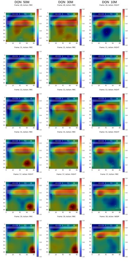
24      CHAPTER 4. METHODOLOGY

a specific action.

There is no predefined strategy on how to evaluate how well an explanation
captures the reasoning of the system. Petsiuk, Das, and Saenko [20] used
Insertion-Deletion to test how well an explanation provided by RISE actually
explains the system for image classification problems. For the RL setting in
this study, Deletion was used to evaluate the explanation provided by the heat
maps. The intuition of this is that if the explanation is good, removing features
identified as important would result in the agent not being able to achieve good
scores playing the game. One could then let the agent play a game and for each
frame generate a heat map pointing to the most important features associated
with the action chosen. The feature identified would then be removed from
the frame, and the agent would be presented with the frame where the feature
has been removed. From this the agent would choose a new action and the
action would then be fed to the game environment which computes a score
based on the action and switches its state. This is then repeated for all frames
in the game sequence until the game either finishes or is lost. The scores and
standard deviation are measured over several games and if there is a sharp per-
formance drop when removing important features identified, the explanation
has high relevance.

4.2      Training DQN Agents
This section provides the outline for how the Atari environment was set up
in which the agents were trained, as well as how the DQN agents and their
extensions were configured. The section also gives an account for the training
setup used for training each of the DQN agents, and how they were chosen
based on evaluation scores.

4.2.1     Agent Configuration and Training Setup
To be able to easily observe any strategies used by RL agents, an environ-
ment with previously observed strategies was chosen. For this, the Atari-
Breakout [27] game was chosen. In this environment, the agent is tasked with
moving a paddle left or right to intercept a ball bouncing between the walls
and bricks. The agent scores points by shooting the ball onto the bricks, and
in this way destroying them, which rewards the agent with one point per brick
destroyed. Agents have been observed to shoot the ball towards the sides of the
playing field, digging tunnels at the sides, where the ball can be shot through
CHAPTER 4. METHODOLOGY                  25

to destroy the remaining bricks by bouncing the ball between the bricks and
the ceiling of the playing field. Stable-Baselines [33] has a built-in interpreter
for several Atari games based on that of Brockman et al. [27]. It generates a
vectorized environment where four consecutive pixel frames are stacked and
fed to the RL agent. This stacking is done so that the RL agent is able to dis-
cern the speed and direction of moving objects in the environment, which is
otherwise impossible for the agent to detect from just one frame. Each frame
is preprocessed so that it has a shape of 84 × 84 pixels and is converted to
gray-scale. During training the random number generator for the environment
had its seed set to 0.

For the Q-network of the DQN algorithm, Stable-Baselines has several im-
plementations that can be imported. The one chosen for this project was the
same as the one implemented by Mnih et al. [35]. Optimization during train-
ing was done using the Adam optimizer [36] with a learning rate of 0.00001.
To ensure that the agent explores enough during the early stages of training,
epsilon-annealing was used. The initial  was set to 1.0 and then decreased to
0.01 over 10% of the total training time. The size of the replay memory [29]
was set to 100000. The agent was trained for 50000000 time steps, where one
time step is equivalent to one pixel frame. The parameter updates are done ev-
ery fourth time step and the target network updates are done every 10000 time
steps. For each update a mini-batch is drawn from the replay memory and the
update is done for all mini-batch samples, where the mini-batch size was set
to 32. The first update during training is done after 100000 time steps. This
is done to ensure that enough uncorrelated samples have been stored in the
replay memory before training begins. The agent plays several hundred thou-
sand episodes during training, where one episode is defined in three ways:

   1. The agent has lost all five lives, where a life is lost when the agent is
      unable to intercept the ball and it subsequently goes out of bounds.

   2. The agent has reached the maximum number of time steps (10000) for
      an episode.

   3. The agent has successfully destroyed all bricks.

After each episode the environment is reset and new observations are drawn,
which is repeated until the maximum number of training time steps have been
reached. Agents were saved with regular intervals, and the trained agents were
then evaluated to choose three suitable agents for the XAI evaluation. The eval-
uation of agent performance was done by letting each agent play 100 episodes
26 CHAPTER 4. METHODOLOGY
that were randomly initiated. The mean score and standard deviation over all
episodes were calculated for each agent, and the three agents with the best
mean score and standard deviation were chosen. The three agents that were
chosen are presented in Table 4.2.1. The reasoning for choosing three different
agents that have varying amounts of training is that one might be able to see
how agents with varying amounts of skill solve the game. Each of the agents
had Double DQN [30] and Dueling DQN [31] architectures enabled and used
a discount factor γ of 0.99.
Agent name #training steps Mean Score std
DQN_10M 10 000000 98.52 84.93
DQN_30M 30 000000 257.33 125.18
DQN_50M 50 000000 374.38 52.02
Table 4.1: Performance of DQN agents trained for various amounts of time
steps.
4.3 RISE and Generating Heat Maps
This section introduces the experimental setup of the chosen XAI explainer
and how the explanations were generated.
4.3.1 Setting up RISE
RISE is a very simple algorithm to implement since it only uses the input-
output of the model that is to be explained. Each observation is copied and
N number of random masks are generated for each observation. The masks
and the observations are then element-wise multiplied resulting in N masked
observations. These masked observations are then fed to the agent. For each
of the masked observations the importance weight is stored as the Q-value that
corresponds to the action that was originally selected by the agent. The reason
for selecting the Q-value rather than the probability, is that, for many agents
the probabilities for actions are very similar between observations and there
is little deviation from the mean value. So using the Q-values gives a larger
importance ratio and produces better heat maps. RISE has four hyperparam-
eters that can be set for the different problems. The number of masks N , the
size of the smaller cell that is to be up-sampled (h × w) and the probability p
of setting elements of the smaller cell to one. The values for these parameters
were found empirically by generating about 100 heat maps for each agent andCHAPTER 4. METHODOLOGY 27 observing what values seem to give the best heat maps. The values used for all agents were N = 8000, h = w = 6 and equal probability of setting a pixel to 1 or 0, that is, p = 0.5. The smaller cells were up-sampled to the image size of 84 × 84 by using bi-linear interpolation, as suggested by Petsiuk, Das, and Saenko [20]. Since the agents use observations that are four pixel frames stacked in a sequence, the same mask is applied to all four frames per observa- tion. This is done so that the agent will not be able to discern features if they are present in a frame that has not been masked. 4.3.2 Generating Heat Maps Generating heat maps for the three agents is straightforward but very time- consuming. On average generating heat maps for a full episode of a game takes a minimum of 6 hours. Each agent is allowed to play one episode, that is, either destroying all bricks, losing all lives or reaching the maximum number of time steps allowed for a game. Each agent plays one game where the seed of the Atari environment set to zero. The reasoning for letting all agents play one game in common is to be able to do a comparison between how different agents with varying degrees of skill behave. Each of the agents then play an additional three games where the seed is a randomly generated integer between 0 − 1000. Each of the agents had heat maps generated for a total of four games to be used for comparisons and t-SNE clustering. 4.4 Evaluating Explanation Using Deletion As explained, the intuition for using Deletion is to test how well an explanation captures what the agent finds important in its decision making. The Deletion scheme is set up so that each agent first plays a game where no pixels have been removed, saving these as the baseline performance. Then iteratively, the agents play a game where 5% of the most important pixels are removed from each observation according to the corresponding heat map. Next iteration 10% of the most important pixels are removed for the duration of the game. This is repeated, increasing the amount of pixels removed by 5% for each game up until 100% where the agent plays a game with all pixels removed. Removing a pixel means setting its value to 0. For the black and white observation means that the pixel value is set to the same value as the background. This procedure of letting the agent play games with various amounts of pixels removed is repeated four times per agent and the results are then averaged over these four games.
You can also read