Estimating density of mountain hares using distance sampling: a comparison of daylight visual surveys, night-time thermal imaging and camera traps ...
←
→
Page content transcription
If your browser does not render page correctly, please read the page content below
Wildlife Biology 2021: wlb.00802
                                                                                                                  doi: 10.2981/wlb.00802
                                                                                      © 2021 The Authors. This is an Open Access article
                                                      Subject Editor: Luca Corlatti. Editor-in-Chief: Ilse Storch. Accepted 27 April 2021

Estimating density of mountain hares using distance sampling: a
comparison of daylight visual surveys, night-time thermal imaging
and camera traps

Carlos P. E. Bedson, Lowri Thomas, Philip M. Wheeler, Neil Reid, W. Edwin Harris,
Huw Lloyd, David Mallon and Richard Preziosi
C. P. E. Bedson (https://orcid.org/0000-0001-6489-1138) ✉ (carlosbedson@outlook.com), H. Lloyd, D. Mallon and R. Preziosi, Dept of Natural
Sciences, Manchester Metropolitan Univ., UK. – L. Thomas, Faculty of Biology, Medicine and Health, Univ. of Manchester, UK. – P. M. Wheeler,
School of Environment, Earth and Ecosystem Sciences, The Open Univ., Milton Keynes, UK. – N. Reid, Inst. of Global Food Security (IGFS),
School of Biological Sciences, Queen’s Univ. Belfast, Belfast, Northern Ireland, UK. – W. E. Harris, Dept of Agriculture and Environment, Harper
Adams Univ., Newport, Shropshire, UK.

        Surveying cryptic, nocturnal animals is logistically challenging. Consequently, density estimates may be imprecise and
        uncertain. Survey innovations mitigate ecological and observational difficulties contributing to estimation variance. Thus,
        comparisons of survey techniques are critical to evaluate estimates of abundance. We simultaneously compared three meth-
        ods for observing mountain hare Lepus timidus using Distance sampling to estimate abundance. Daylight visual surveys
        achieved 41 detections, estimating density at 14.3 hares km−2 (95%CI 6.3–32.5) resulting in the lowest estimate and
        widest confidence interval. Night-time thermal imaging achieved 206 detections, estimating density at 12.1 hares km−2
        (95%CI 7.6–19.4). Thermal imaging captured more observations at furthest distances, and detected larger group sizes.
        Camera traps achieved 3705 night-time detections, estimating density at 22.6 hares km−2 (95%CI 17.1–29.9). Between
        the methods, detections were spatially correlated, although the estimates of density varied. Our results suggest that daylight
        visual surveys tended to underestimate density, failing to reflect nocturnal activity. Thermal imaging captured nocturnal
        activity, providing a higher detection rate, but required fine weather. Camera traps captured nocturnal activity, and oper-
        ated 24/7 throughout harsh weather, but needed careful consideration of empirical assumptions. We discuss the merits and
        limitations of each method with respect to the estimation of population density in the field.

        Keywords: camera traps, cryptic animals, distance sampling, population monitoring, survey methods, thermal imager, uplands

In a global era of biodiversity crisis, conservation monitor-             servation. Reliable estimates of mountain hare population
ing which allows us to establish trends in wild animal abun-              density are important to inform conservation assessments
dance, is essential. The provision of reliable census estimates           and to evaluate the impact of anthropogenic disturbance
are considered vital to guide management interventions                    on population numbers (e.g. impact of roadkill or control
aimed at protecting vulnerable species (Krebs 1989). Effec-               efforts on grouse moorland). Yet hares are mostly nocturnal
tive surveys must be designed to reflect species distribution             mammals and can be difficult to detect (Newey et al. 2011,
and life history traits which may affect animal detection.                Petrovan et al. 2011). Despite having a white pelage in win-
Studies must comprise sites which represent the range of                  ter, hares are adept at hiding by day in rough vegetation:
habitats, climate and topography occupied by the target spe-              they lie motionless, flattening to 15 cm height, sometimes
cies and this will both inform and constrain survey methods               in shallow depressions, burrows or amongst rocks and even
(Sutherland 2006).                                                        fleeing unseen. Hares emerge at night to feed (Hewson and
    The mountain hare Lepus timidus is Britain’s only native              Hinge 1990, Harris and Yalden 2008) and consequently
lagomorph and an icon for upland habitats and their con-                  daytime observation is characterised by low detection rates
                                                                          (Dingerkus and Montgomery 2002).
                                                                              Surveying elusive or nocturnal animals is particularly
This work is licensed under the terms of a Creative Commons
Attribution 4.0 International License (CC-BY) . The license permits                often experience poor weather. Mountain hare habitats are
use, distribution and reproduction in any medium, provided the            also frequently rugose and difficult to access, creating safety
original work is properly cited.                                          issues for monitoring, especially at night. Mountain hares

                                                                                                                                              1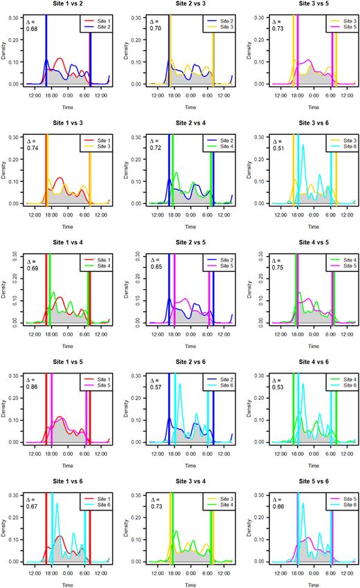
frequent low hills, gullies and deep vegetation, making          Methods and materials
detection difficult (Newey et al. 2018). Snow may hamper
daytime observations of white camouflaged mountain hares.        Study site
Effective monitoring therefore requires multiple observation
points and benign weather.                                       Surveys took place at Holme Moss, a large hill, elevation
    Considering the suite of study methods available for         582 m a.s.l., situated in the north of England, UK (Fig. 1).
wildlife monitoring, mark–recapture is regarded as the most      Mountain hares were once native to England yet became
reliable for hares (Boulanger and Krebs 1994). However,          extinct ~ 6000 years ago (Yalden 1971). They were rein-
addressing welfare concerns surrounding the capture and          troduced to Holme Moss in the 1870s for sport shooting
handling of animals is resource intensive, particularly in       (Stubbs 1929, Yalden 1971). In this area historic records
rough terrain, making this method expensive and impracti-        suggest the number of 1-km squares occupied by mountain
cal. Faecal pellet counts can provide a useful index in areas    hares as ranging from 16 (Yalden 1971) up to 35 (Mal-
of high hare density, assuming constant accumulation rates       lon et al. 2003). This group of hares is potentially partially
(Newey et al. 2003). Whilst it is also possible to obtain DNA    isolated from other populations elsewhere in the area by res-
from faecal pellets for genetic population monitoring with       ervoir systems and major road networks. Whilst sightings of
molecular mark–recapture, both plant material in the pellets     mountain hares on Holme Moss have been particularly fre-
and fast decay rates can reduce PCR effectiveness, requir-       quent in the past (Mallon et al. 2003), farmers and landown-
ing larger sample sizes and greater field and laboratory work    ers report perceived declines across the site in the last decade.
and costs (DeMay et al. 2013). Direct observation methods        The local density on Holme Moss has never been formally
by day, such as line transect sampling, are commonly used        quantified. Holme Moss comprises a flat plateau with peat
yet are vulnerable to achieving fewer observations when such     gullies and steep sided valleys (Fig. 1) (Tallis 1987). The area
predominantly nocturnal animals remain undetected (Buck-         consists of blanket bog vegetation dominated by heather
land et al. 2001). Areas of low density may result in low        Calluna vulgaris, bilberry Vaccinium myrtillis and cotton
encounter rates and wide variance in estimates (Newey et al.     grass Eriphorum spp. Over the last 200 years habitat condi-
2018). Night-time spotlight surveys may miss animals as          tions have deteriorated as both acid rain caused peat layer
they rely on eyeshine reflections, and frequently sample         reduction and intensive sheep grazing led to widespread
along roads which animals may avoid and which locations          vegetation loss (Anderson and Shimwell 1981). Most of the
represent only a small fraction of upland habitat (Reid et al.   hill is managed by the RSPB Dove Stone reserve engaged in
2007, Reid and Montgomery 2010). Thermal imaging                 blanket bog restoration.
reduces false negatives by increasing target detections, con-        The study focused on the entire blanket bog plateau of
trasting body heat against a cold backdrop at night (Havens      Holme Moss, where elevation was above 335 m i.e. the
and Sharp 2016) but if the aim is to estimate density it         lower elevation range of mountain hare occurrence (Yalden
also requires a means to determine distance to the object in     1971), and as limited by major roads to the north and east
darkness. Camera trapping provides a greater continuous          and different habitats to the south and west. This comprised
survey effort including during night peak activity periods       49 km2. Within this area we selected a smaller 5 × 5 km
thus increasing total numbers of detections (Caravaggi et al.    central area for daylight visual surveys, thermal imager and
2018), and with virtually no observer field presence to dis-     camera trap surveys. This considered the area that could be
turb animals (Sollman 2018).                                     covered on foot by two full time staff conducting field logis-
    In this study we compared three survey methods of            tics: Holme Moss is largely pathless, often hazardous under-
mountain hares in upland habitat to estimate density             foot. Winter day lengths are short. The location of the 5 ×
and considered factors relating to spatial variation of hare     5 km area was chosen to be central, equidistant from roads
detections: 1) daylight visual surveys, 2) night-time ther-      and habitat edges, avoiding edge areas frequented by the
mal imaging point transects and 3) fixed position camera         public, thereby reducing camera theft risk, though accepting
traps. We analysed data from each method using compa-            this choice of centroid might cause bias. Within this area
rable distance sampling models to estimate density and           we then randomly selected (R-package ‘sample’) 5 × 5 1-km
associated precision. For each method we recorded sur-           squares as the locations for random cluster samples of points
vey effort, observations, distances to target animals and        and transects, being representative of the flat blanket bog.
group sizes as inputs to estimate density. As camera trap        The location of an additional sixth site was also randomly
distance sampling methods are relatively recent, we also         selected, yet at the request of wildlife agencies we altered its
explored how different assumptions of space, time and            shape to comprise a narrow long strip to facilitate monitor-
animal behaviour affected density estimates. Since actual        ing of an historic high density area (Mallon et al. 2003),
densities or population size were not known, we could            accepting this might bias results. Contemporary density
not be certain which density estimate of the three meth-         and distribution of hares was unknown. The 1-km size of
ods might be closest to the truth. Nonetheless the overall       each study site enabled comprehensive continuous observa-
precision of parameters and estimates could be compared.         tion of terrain, detecting potential changes in hare occur-
We compared variation of estimates among methods and             rence over a few hundred metres. Hare home ranges can be
survey sites, the effect of terrain type and how detection       small (0.1–0.8 km2), non-territorial, overlapping and hares
rates changed throughout the study period. We evaluate           sometimes group together (Hewson and Hinge 1990, Hul-
the merits and assumptions of each method relative to our        bert et al. 1996, Rao et al. 2003, Harrison 2011). The small
findings, to inform study design decisions for conservation      1-km site scale facilitated efficient management of camera
monitoring.                                                      arrays and enabled observers to learn of local topography and

2
Daylight visual surveys

                                                                      Daylight visual surveys took place using line transects fol-
                                                                      lowing Ordnance Survey (2015) Explorer Map 1 grid lines
                                                                      which bounded each survey site (Fig. 1). Transects were
                                                                      square circuits (Buckland et al. 2001, p. 237), intended to
                                                                      alleviate detection bias arising from a low winter sun posi-
                                                                      tion when walking different cardinal directions, wind or
                                                                      local topography effects, whilst enabling efficient use of sur-
                                                                      vey time. Whilst surveys were conducted only during good
                                                                      visibility, poor weather and persistent snow cover limited
                                                                      the survey opportunities to only one visit per site transect.
                                                                      Observer routes were guided by a handheld GPS. A slow,
                                                                      measured walk was used (~ 1 km per hour), with frequent
                                                                      scanning of the landscape using binoculars (Fig. 2). The
                                                                      location of each mountain hare was recorded, measuring
                                                                      radial distance from the observer with a laser range finder
                                                                      (maximum range 1100 m) and angle using a compass. These
                                                                      measurements allowed the calculation of the perpendicular
                                                                      distance of sightings from the line, and also enabled the loca-
                                                                      tion of each hare to be mapped. During these surveys, con-
                                                                      ducted when there was no snow, mountain hares bore white
                                                                      pelage contrasting against the green and brown moorland.
                                                                      Hares were often lying-up and not detected until within 30
                                                                      m range (Fig. 2). Whilst some hares fled from the observer,
                                                                      this occurred within the range of vision, so distance and
                                                                      angles were measured to point of origin.

                                                                      Night-time thermal imaging

                                                                      We conducted nocturnal surveys at point transect locations
                                                                      using an Armasight Command 336 HD 30 Hz 75 mm
                                                                      biocular (two view lenses) thermal camera, with a range of
                                                                      2 km, and a refresh rate 30 Hz which enabled species iden-
Figure 1. Location of Holme Moss study site, north west England,      tification of moving animals (Fig. 2). The camera was fit-
Great Britain. Aerial photo origin is OS SE 401398 and shows
extent of Holme Moss massif, above 335 m elevation, bounded to        ted with an Advanced Modular Range Finder 2200 which
north and east by major roads. The hill summit is indicated by the    operated in darkness. In trials, distances up to 1.8 km could
black square. Survey locations are shown, with site numbers. Sites    be measured. This assemblage was mounted on a tripod at
1–5 are 1 km squares. Site 6 is the narrow polygon running north      each point location each spaced ~333 m apart (about the
to south between sites 2 and 5. Daylight visual transects were the    diameter of a single hare home range) along the same 1-km
perimeter of 1-km square, except site 6 being a near trapezoid        grid lines used during daylight visual surveys (Fig. 1). Thus,
shape. Thermal imager points were 333 m apart as were camera          whilst a different survey method was used at a different time
traps, though with some minor deviations for topography, standing     of day, survey sites were the same. Surveys did not occur at
water or perceived theft risk. Note: one thermal imager point was
used in site 4 and repeated ~30 m away in site 5; 87 of 91 camera     a location that had received a visit that day for other survey
site locations are shown as 4 pairs of camera trap sites overlap; 2   purposes, to ensure hares had not been disturbed. Points at
were moved ~30 m mid-term because of rising standing water; 2         sites 1–4 were visited 2–3 times over the winter; points at
were moved ~30 m avoiding perceived theft risk. Three cameras         sites 5 and 6 were visited once only.
were stolen from site 3 and one from site 6; their points are not         Surveys were conducted one hour after sunset with clear
shown, no data was recorded at those locations. Aerial photograph:    visibility though some surveys were curtailed by fog or high
Digimap sourced June 2019 from Digimap Ordnance Survey Col-           winds. Some surveys occurred on snow which assisted detec-
lection: Getmapping aerial imagery.                                   tion of hares. Walking by night from point to point took
                                                                      approximately 20–30 min. A red-light head-torch was used
hazards, prior to subsequent night surveys for thermal imag-          by observers to guide the way between points, minimising
ing. Within the six study sites, we chose transect and point          disturbance. Hares were seen twice only during transit. Once
layouts which would cover the same locations, to capture the          set up, the thermal imager assemblage was immobile; care
same local variation. However some of the survey locations            was taken to situate it with the best field of view within 20
between methods differed slightly to account for the differ-          m of the GPS point. Whilst setting up the thermal imager
ent observation ranges of equipment. Surveys occurred from            vantage point no hares were observed within 30 m. Surveys
November 2017 to May 2018 (Supporting information).                   at each point transect consisted of complete 360° field scans
The period was characterised by exceptionally severe weather          and typically took 10–20 min per point. Extensive practice
including seven heavy snowfalls (UK Met Office 2019).                 with the thermal imager using the setting ‘white hot’ ensured

                                                                                                                                   3
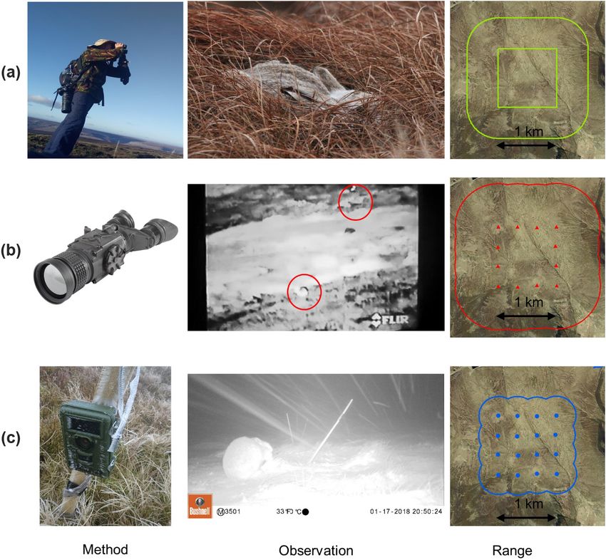
Figure 2. Photographs showing the three different methods. (a) Daylight visual surveys, (b) thermal imager, (c) camera trap. Left column
shows the observation equipment. Central column shows each method’s typical sighting of a mountain hare. Right hand column displays
example survey location at site 1 for each method, duly surrounded by a buffer: measured to the furthest visual point (532 m) for daylight
visual surveys; (740 m) thermal imager; for camera traps, buffer is portrayed to 333 m of each camera, the assumed home range of local
mountain hares.

identification of hares which were easily distinguished from           were sited at the same locations as daylight visual surveys
grouse Lagopus lagopus whose feathers blocked heat radia-              and thermal imaging surveys, along the Ordnance Survey
tion except for beaks, and foxes Vulpes vulpes that were much          map bounding grid lines of each site as well as several placed
larger (Fig. 2). For each detection, angle and distance mea-           in the centre of each square for fuller coverage. Distances
surements were recorded as during daylight surveys. Three              between cameras were thus 333 m, again this being the
sightings of leverets were excluded, to estimate adult densi-          assumed home range diameter of mountain hares. Cameras
ties only.                                                             were 14 MP Bushnell NatureView No Glow, set to high sen-
                                                                       sitivity. Pilot tests showed a large number of false detections
Camera traps                                                           would be elicited (wind blown vegetation). Capturing video
                                                                       might expend battery and memory capacity before revisits
We placed between 12 and 16 camera traps at each of the                by staff and also make image review time excessive. Thus
six survey sites (Fig. 1). Due to logistical constraints, camera       cameras were instead set to trigger at 1 s intervals with time-
traps were deployed at site 1 before being moved sequentially          stamp recording. Camera functioning was evidenced by a 12
to site 6 (they could not be deployed simultaneously). Cam-            hourly ‘field scan’ setting. Cameras were installed on posts at
eras were left in situ for two to five weeks at each site (Sup-        40 cm above ground level (Fig. 2) set facing north to avoid
porting information), depending on weather conditions,                 false triggers by sun movements. Bamboo canes were placed
camera performance and perceived risk of theft. Cameras                in a line at intervals of 2, 4, 6, 8 and 10 m in front of each

4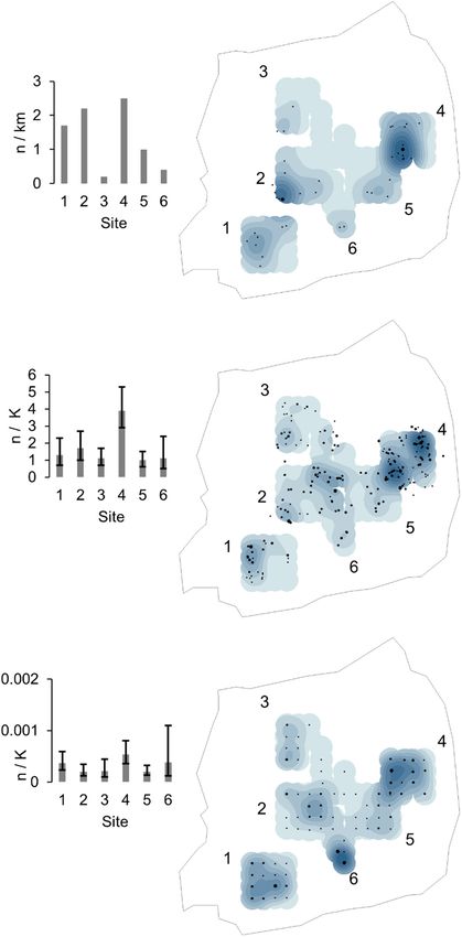
camera to measure the distance of each hare to the camera         2001). As sequences of camera trap detections occurring
at 1 m spacing (Fig. 2) (Hofmeester et al. 2016, Howe et al.      over several seconds were not independent we calculated the
2017). Photos were managed with TIMELAPSE 2 (Univer-              overdispersion factor ( Ĉ ) and used log likelihood (ℒ) to cal-
sity of Calgary, Canada) software. Images were catalogued by      culate QAIC, i.e. the two step model evaluation approach of
location, date and time.                                          Howe et al. (2018).
    We reviewed the frequency of camera images of hares
and considered one second as representing the survey snap-        Statistical analysis
shot period (‘k’) for point counts following advice from
Howe et al. (2017) to use time periods < 3 s. For each posi-      Descriptive statistics were tabulated for a suite of param-
tive detection we recorded each individual’s radial distance      eters capturing survey effort, numbers of detections, detec-
to camera for distance sampling estimation. In a few cases        tion distances and encounter rates for each survey method.
with darkness or poor focus this was difficult to determine.      Based on the surveys’ efforts and results, we calculated and
Images showed some hares, having appeared in the camera           compared the level of effort to achieve a required precision
zone, inspected the distance marker cane or the camera itself.    of density estimate, using formulae from Buckland et al.
We considered this attraction behaviour, known to contrib-        (2001). Spatial autocorrelation of sightings (encounters)
ute to sampling bias (Corlatti et al. 2020) and discounted        was examined with kernel density maps of detections using
those images.                                                     ArcGIS ver. 10.6.1 and tested using Moran’s I index for
    Unlike daylight visual surveys and night-time thermal         each survey method. Comparison of sighting densities
imaging where surveys were time limited, camera traps can         between the three methods was assessed by Pearson cor-
make detections 24/7. No detections are likely to be made         relation of the kernel density maps. ArcGIS was used to
when an animal is resting and so survey effort during day-        map topographical gullies plotted as shapefile vector data
light is highly vulnerable to false negatives, potentially low-   (Ordnance Survey 2018), converted into a raster of gully
ering average density estimates. We defined the hare activity     density using the line density and polygon to raster tool-
cycle using a frequency histogram of detections against each      box functions (100 m cell size). The relationship between
hour of the 24-h cycle, fitting a smoothed density function       hare encounter rates and gully density was examined using
for each site according to standard methods (Ridout and           linear regression for each survey method. Temporal trends
Linkie 2009, Rowcliffe 2014). Conservative approaches may         in camera trap encounter rate were examined using a sepa-
consider analysis which refers to the peak diel periods when      rate general linear mixed model (GLMM) fitting ‘Site’ as
~ 50% of activity occurs (Frey et al. 2017) or ≥ 55% activity     a random factor to account for multiple observations per
(McGowan et al. 2019). However our camera sites occurred          site (multiple days recording) and the sequential deploy-
over four months, winter solstice to spring equinox, when         ment of cameras at different sites, and with ‘days since start
nights became shorter. Thus when assessing the activity fre-      of survey’ fitted as fixed effect. Daily detections followed
quency densities and potential correlations between sites         a negative binomial distribution. Statistical analyses were
with R-package ‘overlap’ (Meredith and Ridout 2020) we            conducted using R ver. 3.6.1 () and
found different timings of bimodal activity patterns. For         R-package ‘lme4’ (Bates et al. 2015) for linear models fol-
consistency we therefore defined the night-time period as         lowing Crawley (2002).
sunset-to-sunrise at the mid-term date per site (HM Nauti-
cal Almanac Office 2019) thought to provide accurate lev-
els of activity (Vazquez et al. 2019). This night-time period     Results
encompassed > 95% of all camera trap detections.
                                                                  Daylight visual surveys
Distance sampling
                                                                  Over five days, the six sites were surveyed for a total of 26 h
Data from each method were analysed using software dis-           (Table 1, Supporting information). Daylight visual line tran-
tance ver. 7.2 (Thomas et al. 2010) including site, survey        sect surveys required 3–7 h per transect which were 4–8 km
effort, number of detections, distance to each detection and      in length. Mean radial detection distance was 152 m and the
cluster size (Buckland et al. 2001).                              furthest was 532 m. Thus, the survey rate was 0.98 km2 per
    Daylight visual surveys were analysed using ‘line transect’   hour (Table 1). In total, 41 mountain hare detections were
protocols and thermal imaging as ‘points’, each assuming          recorded with 1 detection every 0.63 h (~38 min). During
360° field-of-view. Camera trap surveys were also analysed        daylight hours 95% of the detections were of solitary indi-
as points; however survey effort had a restricted 42° field-      viduals, the remainder being pairs (Table 1). Owing to hid-
of-view of each camera, thus distance analysis for camera         ing and flushing behaviour of hares, 16 detections occurred
trap data multiplied total effort ‘k’ by 42/360 following         within 30 m of the observer. Thus to enable a choice of
Howe et al. (2017). Model fit was optimised in each case          detection function models, we truncated data at 100 m
using truncation of the most distant detections and variable      and assigned observations to bins at 5, 10, 20 and 100 m
bin width as appropriate. Models assessed included uniform,       (Table 2). Candidate models showed high χ2 goodness-of-
half-normal and hazard-rate models; and model averaging           fit (GOF) values (> 0.31) with similar detection probabili-
was also considered. Models were evaluated by referring to        ties. The half-normal model reported lowest AIC, p = 0.28,
Akaike information criterion (AIC), χ2 goodness-of-fit test       (cv) = 0.20 and was selected for density estimation. (Table
values, detection probability (P) values and coefficient of       2, Fig. 3a). Following data truncation, encounter rate was
variation (P CV) using established methods (Buckland et al.       0.82 km−1, (cv) = 0.31 and observations were singles making

                                                                                                                                5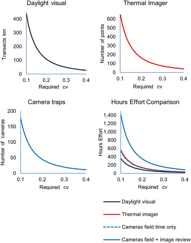
6
    Table 1. Descriptive summary of sampling effort, detections and their distance from the observer and surveyed area (based on furthest detection distance) for daylight visual surveys, thermal imaging
    and camera trapping. Samples and detections are total values before truncation. Per method ‘Summary’ rows: Σ = column total; x = column mean. All camera trap values based on night-time (informed
    by Fig. 4). Calculation of area surveyed at each site for cameras = (further detection distance per site)2 × π × camera field of view restriction (42/360) × number of cameras per site. The survey rate (km2
    per hour) for camera traps is not calculated as they are considered to be in continual operation.

                                                                                    Mean cluster    Mean detection        Furthest        Detections per      Hours to 1st     Surveyed area       Survey rate
    Method (survey units)           Samples           Hours effort   Detections        size          distance (m)       detection (m)         hour             detection           (km2)         (km2 per hour)
    Daylight visual surveys Sample units = Transect length km
      Site 1                          4.62                  3            8           1.00             149                305                    2.67              0.38             3.11                1.04
      Site 2                          4.82                  4           11           1.09             220                446                    2.75              0.36             4.92                1.23
      Site 3                          4.71                  4            1           1.00             192                192                    0.25              4.00             1.93                0.48
      Site 4                          4.70                  4           12           1.08             172                532                    3.00              0.33             5.89                1.47
      Site 5                          4.89                  4            5           1.00               87               362                    1.25              0.80             3.95                0.99
      Site 6                          8.16                  7            4           1.00               94               263                    0.57              1.75             4.51                0.64
      Summary                       Σ = 31.91            Σ = 26      Σ = 41        x = 1.03          x = 152          x = 350.0               x = 1.75          x = 0.63         Σ = 24.31           x = 0.98
    Thermal imaging Sample units = points (number of replicates in brackets)
      Site 1                         12 (20)               16           26           1.34              185               508                    1.63              0.62            16.21                1.01
      Site 2                         12 (22)               22           38           1.31              256               612                    1.73              0.58            25.88                1.18
      Site 3                         12 (27)               19           30           1.43              218               500                    1.58              0.63            21.20                1.12
      Site 4                         12 (22)               20           87           1.44              270               682                    4.35              0.23            32.14                1.61
      Site 5                         12 (12)               10           12           1.08              436               740                    1.20              0.83            20.64                2.06
      Site 6                         11 (11)               10           13           1.38              220               528                    1.30              0.77              9.63               0.96
      Summary                     Σ = 71 (114)           Σ = 97      Σ = 206       x = 1.33          x = 264          x = 595.0               x = 1.96          x = 0.47        Σ = 125.71           x = 1.32
    Camera traps Sample units = number of cameras (total camera nights in brackets) [hours per night in square brackets]
      Site 1                      16 (287) [17]          4879          768           1.00             2.33                 9                    0.15              6.35           0.000475               –
      Site 2                      16 (376) [17]          6392          550           1.00             2.60                10                    0.08            11.62            0.000586               –
      Site 3                      12 (148) [16]          2368          213           1.00             1.92                 6                    0.09            11.12            0.000158               –
      Site 4                      16 (331) [15]          4965        1128            1.00             2.91                12                    0.23              4.40           0.000844               –
      Site 5                      16 (386) [14]          5404          479           1.00             2.60                 8                    0.09            11.42            0.000375               –
      Site 6                      15 (272) [13]          3536          573           1.00             2.41                 9                    0.16              6.17           0.000445               –
      Summary                Σ = 91 (1800) [varying] Σ = 27 544     Σ = 3705       x = 1.00         x = 2.46             x =9                 x = 0.13          x = 8.51       Σ = 0.002884             –
1.00 cluster size (Table 3). The contribution to variation of             ing 5112 images of mountain hares per 1 second snapshot
density estimate was encounter rate (72.5%) and detection                 window. The remaining images were false triggers: wind-
probability (27.5%).                                                      blown vegetation or other animals e.g. foxes, stoats Mustela
                                                                          erminea. Of these images 1329 showed hares attracted to
Night-time thermal imaging                                                marker canes or the camera, so were excluded, leaving 3783
                                                                          separate detection events.
Over eleven nights, a total of 114 point transects located along              Of these, just 78 detections (2%) occurred by day; 3705
the boundary of the six sites were surveyed for a total of 97 h           detections (98%) during night-time, averaging 1 detection
(Table 1, Supporting information). Surveys needed 5–7 h to                per 8.5 h (Table 1). Night-time showed the largest activity
cover up to 12 points per night. Mean detection distance was              peak after sunset, followed by moderate activity periods, and
264 m and the furthest was 740 m. Thus, the survey rate was               a distinct peak before dawn (Fig. 4). This pattern was similar
1.32 km2 per hour or 0.00587 km2 (i.e. 5870 m2) per point                 at each site for the study duration: activity occurring over
(Table 1). In total, 206 mountain hare detections were made               17 night hours late November (site 1), compressing into
with 1 detection every 0.47 h (~28 min). During darkness                  13 night hours late March (site 6). However the timing of
74% of detections were solitary individuals, the remainder                night-time activity peaks differed between sites. The highest
groups of up to 8 hares (Table 1). For modelling, detections              correlation was 86% between sites 1 and 5; the lowest cor-
were truncated at 350 m. All candidate detection functions                relation 51% between sites 3 and 6. Based on night-time
achieved model fit (Table 2). The hazard-rate model had low-              detections, the mean detection distance was 2.4 m and the
est AIC and highest χ2 GOF = 0.78 with P = 0.34, (cv) = 0.21              furthest was 12 m, and 95% of detections were within 5
and was selected for density estimation (Fig. 3b). Following              m of the camera (Table 1). Thus, the survey rate averaged
data truncation encounter rate was 1.33 k−1, (cv) = 0.12 and              0.0003 km2 (i.e. 30.0 m2) per camera (Table 1). Night-time
estimated cluster size 1.31, (cv) = 0.04 (Table 3). The con-              detections for distance analysis modelling assessments were
tributors to variation of density estimate were encounter rate            allocated to bins at 1, 2, 3–4 and 5 m (Table 2). Having cal-
(24.5%), detection probability (73.9%), cluster size (1.6%).              culated QAIC and ( Ĉ ) for candidate models, the latter was
                                                                          lowest for the hazard-rate model at 1.8 and χ2 GOF = 0.18,
Camera traps                                                              thus was selected for reporting with P = 0.17, (cv) = 0.03
                                                                          (Table 2 Fig. 3c). Camera trap encounter rate was 0.00030
Over four months, a total of 91 camera locations were                     k−1, (cv) = 0.14 (Table 3, Supporting information). Cluster
installed throughout the six survey squares (total = 1800                 size was 1.00, (cv = 0.01). The contribution of variation to
days i.e. 27 544 night hours) (Table 1, Supporting infor-                 the density estimate was encounter rate (95.4%) and detec-
mation). In total, 107 000 images were captured, retriev-                 tion probability (4.5%).

Table 2. Summary of models showing number of parameters (# para), AIC, Delta AIC, χ2 values, degrees of freedom (df), and χ2 goodness of
fit (GOF), detection probability (P) and co-efficient of variation values (P CV). For camera traps, log likelihood (log ℒ), overdispersion factor
( Ĉ ) and QAIC are shown for assessments of over-dispersed data (Howe et al. 2018). For each survey method, data selections and number
of observations (n obs) are listed. Models selected for subsequent estimations are marked with asterisk *.

                                                            Delta
           Model (key)             # para        AIC        AIC          χ2       df   χ2 GOF       p       P CV
    Daylight visual surveys      Data truncation at 100, bins at 5 m, 10 m, 20 m and to 100 m, n obs = 26
      Uniform + cos                  2            74.3          2.3        0.7    1     0.40    0.31         0.36
      Uniform + polynomial           1            72.3          0.3        0.6    2     0.73    0.30         0.18
*     Half-normal + cosine           1            72.0          0.0        0.4    2     0.82    0.28         0.20
      Half-normal + Hermite          1            72.0          0.0        0.4    2     0.82    0.28         0.20
      Hazard-rate                    2            74.6          2.6        1.0    1     0.31    0.33         0.15
    Thermal Imager               Data truncation at 350 m, n obs = 152
      Uniform + cosine               2         1753.6           0.9       11.2 15       0.73    0.29         0.13
      Uniform + polynomial           3         1755.9           3.3       11.2 14       0.66    0.31         0.12
      Half-normal + cosine           3         1753.9           1.3        9.7 14       0.77    0.32         0.29
      Half-normal + Hermite          1         1757.7           5.0       17.6 16       0.34    0.38         0.09
*     Hazard-rate                    2         1752.6           0.0       10.5 15       0.78    0.34         0.21
                                                                                                                      log ℒ        Ĉ     QAIC
    Camera traps                 Data truncation at 5 m, bins at 1, 2, 3–4, 5 m; n obs = 3506
      Uniform + cosine               1         9371.4      875.2        876.4     2    0.00      0.30        0.01    −4684.6    438.2      12.9
      Uniform + cosine               2         8607.4      111.2        109.3     1    0.00      0.18        0.02    −4301.7    109.3      14.0
      Uniform + polynomial           1        10010.5     1514.3       1598.5     2    0.00      0.38        0.01    −5004.2    799.3      13.6
      Uniform + polynomial           2         9359.1      862.9        863.2     1    0.00      0.30        0.02    −4677.5    863.2      14.8
      Half-normal + cosine           1         8709.6      213.4        255.9     2    0.00      0.17        0.02    −4353.8    128.0      36.3
      Half-normal + cosine           2         8562.5       66.3         68.7     1    0.00      0.12        0.03    −4279.2     68.7      37.7
      Half-normal + Hermite          1         8709.6      213.4        255.9     2    0.00      0.17        0.02    −4353.8    128.0      36.3
      Half-normal + Hermite          2         8710.4      214.2        254.2     1    0.00      0.17        0.05    −4353.2    254.2      38.3
*     Hazard-rate + simple           2         8496.2         0.0         1.8     1    0.18      0.17        0.03    −4246.1      1.8    4721.9
      Hazard-rate + simple           3         8498.2         2.0         1.7     0    0.00      0.17        0.03    −4246.1      –        –

                                                                                                                                               7
Figure 3. Distance sampling detection probability and probability density function histograms for (a) daylight visual surveys (uniform
model with cosine adjustment and data allocated to bins at 5, 10, 20 and to 100 m), (b) nocturnal thermal imaging (hazard-rate model
with simple polynomial adjustment and data truncated at 350 m), (c) camera traps (hazard-rate model with simple polynomial adjustment
and data allocated to bins at 1, 2, 4 and to 5 m.
Comparison of methods down) would require 134 h of field effort and if a manual
image review process was used (e.g. Timelapse software with
Distance sampling models from daylight visual surveys esti- auto-completing data entry, estimating 15 s per image), a
mated density at 14.3 hares km−2 (95%CI 6.3–32.5). Night- further 218 h of desk time (Fig. 5).
time thermal imaging from points estimated density at 12.1
hares km−2 (95%CI 7.6–19.4). Camera trapping estimated Spatial and temporal variation
density was 22.6 hares km−2 (95%CI 17.1–29.9) (Table 3).
Extrapolated to the entire 49 km2 study site at Holme Considering sighting locations per site (untruncated data),
Moss, density estimates suggested a total population of 705 daylight visual surveys showed large differences of sightings
hares (95% CI 311–1597) from daylight visual surveys, 597 (encounter rates) with site 3 lowest at 0.2 km−1 and site 4 high-
hares (95% CI 374–951) from thermal imaging and 1109 est at 2.5 km−1, with a sparse distribution except for sites 2 and
hares (95% CI 839–1467) from camera traps (Table 3). 4 (Fig. 6). Thermal imager observations occurred at a mean
Assessing the density estimates and the effort required to rate from 1.0/point (site 5) to 3.9/point (site 4) (Fig. 6) and
achieve reliable precision i.e. 20% coefficient of variation, appeared to show 2 clumped distributions around site 4 (Fig.
daylight visual surveys would require 109 km of transects; 6). Of the thermal imager points, 99 achieved detections, 15
thermal imagers would require 164 points; and camera did not, indicating mostly widespread presence of hares across
traps would require 45 installations (Fig. 5). Comparing all sites. Camera trap observations occurred at a mean rate from
field effort daylight visual surveys surveying at 1.2 km per 0.0002 k−1 (site 3) to 0.0005 k−1 (site 4), and showed the most
hour would require 89 h effort; thermal imager surveying intense occurrence around site 4 (Fig. 6). Of the 91 cameras,
1.2 points per hour would need 140 h effort. Camera traps 77 achieved detections and 14 made no detection, indicating a
needing 3 h per installation (1 h set up, 1 h revisit, 1 h take widespread distribution though with some negative locations.
8Table 3. Estimates of detection probability, density and abundance obtained from distance sampling analyses for all three survey methods.
Value = point estimate; CV = coefficient of variation; LCL and UCL 95% lower and upper confidence limits. Encounter rate: Daylight visual
n/km = encounters per km; Thermal imager: n/k = encounters per point; Camera traps n/k = encounters per second. Abundance estimate
derived from density value projected to the 49 km2 of Holme Moss.
Method Value CV LCL UCL
Detection probability
Daylight visual surveys 0.28 0.20 0.19 0.42
Thermal imager 0.34 0.21 0.23 0.50
Camera traps 0.17 0.03 0.16 0.18
Encounter rate
Daylight visual surveys (n / km) 0.82 0.31 0.36 1.81
Thermal imager (n k) 1.33 0.12 1.05 1.68
Camera traps (n/k) 0.00030 0.14 0.00023 0.00039
Cluster size
Daylight visual surveys 1.00
Thermal imager 1.31 0.04 1.20 1.44
Camera traps 1.00 0.01 1.00 1.00
Effective strip or radius width (m)
Daylight visual surveys 28.3 0.19 18.9 42.2
Thermal imager 202.5 0.10 165.3 248.2
Camera traps 2.1 0.01 2.00 2.13
Density (hares km−2)
Daylight visual surveys 14.3 0.37 6.3 32.5
Thermal imager 12.1 0.24 7.6 19.4
Camera traps 22.6 0.14 17.1 29.9
Abundance
Daylight visual surveys 705 0.37 311 1597
Thermal imager 597 0.24 374 951
Camera traps 1109 0.14 839 1467
Hare detections were not spatially autocorrelated using ing to under record many hares hiding by day. The method
any survey method (Moran’s Idaylight visual = −0.12, Z = 0.12; did provide sufficient observations to enable monitoring of
Moran’s Ithermal imaging = 0.07, Z = 0.99; Moran’s Icamera traps = relative density but with very wide confidence intervals. By
−0.15, Z = −0.27). Sighting density was strongly spatially night the thermal imager frequently observed single or large
correlated between the three methods (Pearson rdaylight visual ~ groups of hares over the furthest distances and estimated
thermal imager = 0.55, p < 0.001, rthermal imager ~ camera traps = 0.45, density with narrower confidence intervals. However ther-
p < 0.001 and rcamera traps ~ daylight visual = 0.52, p < 0.001 (Fig. mal imaging opportunities were limited by bad weather.
6 and Supporting information). Site 4 was consistently esti- Camera traps monitored constantly and achieved the largest
mated to have the highest sighting density regardless of the number of detections reflecting night time activity of hares,
survey method (Fig. 6). Sites 1 and 2 also had substantial capturing mostly single animals at very short observation
sighting densities. distances. Camera trap density estimates were much larger
Site encounter rates using daylight visual surveys and cam- than for daylight visual sampling and thermal imaging and
era trap surveys were unaffected by gully density but encoun- were more reliable, but were susceptible to many assump-
ter rates using night-time thermal imaging were significantly tions. Notwithstanding differences in detection rates the
negatively associated with gully density (F1,4 = 9.11, β ± locations of sightings from each method were highly spa-
SE = −0.833 ± 0.0009, p = 0.039, r2 = 0.69). Site 4 which tially correlated.
had the highest density estimate of mountain hares, had the
lowest gully density of any site (Fig. 7). Daylight visual surveys
Camera traps ran continuously (24/7) from November
to March. Sequential deployment (accounted for imper- Daylight visual surveys for mountain hares have been criti-
fectly using the random factor of site) reported encounter cised when used in areas of low density or during the day
rates showing a near significant decline by 62% over the four when hares are inactive (Petrovan et al. 2011, Newey et al.
months from 37.6 to 14.3 encounters per day (Fixed effects 2018). Our expectation was Holme Moss would elicit fre-
standardised β = −0.009, z = −1.55, p = 0.12; Random quent occurrences of hares (Mallon et al. 2003), yet we
effects: Site Var = 0.10 SD = 0.324; Fig. 8). achieved very few observations. The small sample size we
achieved was below the minimum required for distance sam-
pling and contained some heaping of detection distances.
Discussion The nature of hiding and flushing hares caused many detec-
tions to occur at short range. Thus, when selecting detec-
Our study compared three survey methods for mountain tion function models, we were obliged to use a smaller data
hares which provided very different kinds of observations set with few, wide bins. This selection may have also pre-
and density estimates. Daylight visual surveys produced the cipitated a narrow effective strip width and this may have
fewest observations, seeing mainly single hares and appear- contributed to the overall density estimate as being higher
9Figure 4. Diel activity at sites showing von Mises kernel densities and pairwise overlaps with other sites. The x-axis shows time of day. The y-axis is the frequency estimate of detections. The overlap of densities, common to each pair of sites, is the shaded grey area below both curves. Overlap coefficient values between compared densities is top left. The mean overlap of all pairwise combinations was 68%; all exceeded 50%. Vertical lines indicate sunrise and sunset times for each site pair; night-time hours reducing with spring onset. Dates of operation: site 1: 24 Nov 2017–18 Dec 2017 (17 night hours); site 2: 11 Dec 2017–11 Jan 2018 (17 night hours); site 3: 9 Jan 2018–25 Jan 2018 (16 night hours); site 4: 25 Jan 2018–9 Mar 2018 (15 night hours); site 5: 16 Feb 2018–30 Mar 2018 (14 night hours); site 6: 9 Mar 2018–30 Mar 2018 (13 night hours). Images produced with R-package ‘overlap’ (Meredith and Ridout 2020) based on Ridout and Linkie (2009). 10
Figure 5. Effort required to achieve a target precision of density estimate, as measured by coefficient of variation. Input to the hours effort
comparison is based on Table 1 and assumes for daylight visual surveys 1.2 km h−1 walked; for thermal imagers 1.2 point h−1 surveyed.
Camera traps assumes cameras are in situ for average 21 days. ‘Camera field time only’ based on 3 h per camera being one installation visit,
one maintenance visit, one retrieval visit. ‘Image review’ time assumes 1176 images per camera achieved with 15 s review time per
image = additional 4.9 h per camera.

than for thermal imaging. This was surprising as one might               Night-time thermal imaging
expect thermal imaging to be observing more such noctur-
nal animals leading to a higher encounter rate and density               This study deployed an advanced thermal imager with
estimate. Although detection probability variation was mod-              mounted laser range finder for measuring distances to object
erate, encounter rate variation was high. Consequently, the              in complete darkness and with point transect protocols.
density estimate possessed wide confidence intervals and                 Whilst seemingly dangerous to walk across moorland by
variation. To achieve reliable estimates, useful for ongoing             night, this could in fact be done as safely as by day, though
monitoring, surveys should achieve 80 or more detections                 slower. However, it was physically difficult to achieve 12 van-
(Buckland et al. 2001). This suggests that studies simi-                 tage points, spaced 333 m apart, in a single night for a single
lar to ours would benefit from replicate surveys to achieve              observer. As the thermal imager was viewed through two
a larger sample size to result in more accurate population               lenses on its internal screen, it provided a 3D image and alle-
density estimates, were this important for monitoring design             viated issues of eye strain. Cold temperatures below −5°C
goals. In retrospect for our own study we might have sac-                flattened batteries within 60 min. Sinking hill fog or increas-
rificed some camera trap management time for more line                   ing winds through some nights, cut surveys short. Ther-
transect surveys. Alternatively, daylight survey effectiveness           mal imaging enabled observations of hares across a broad
might be improved by 3 or 4 observers walking abreast. Day-              landscape, where they exhibited feeding and social behav-
light visual surveys provided an advantage as transect routes            iour. The presence of the observer did not prompt evasive
forced the observer to traverse gullies, opening up fields of            movement. The method worked well on snow. Encounter
view and occasionally enabling sheltering hares to be seen.              rates provided a sample size greater than the ~ 80 detections

                                                                                                                                            11
Figure 7. Map of gullies (lines) with gully density (cells) across the
six study sites at Holme Moss. Numbers denote each study site.
might be within viewing range but hidden in gullies. Future
thermal imaging studies could by day prospect for a large set
of unimpeded vantage points, from which to draw a random
sample to visit by night. Our findings suggested high levels
of precision could be achieved with a logistically manageable
number of points, requiring ~15 nights, assuming favour-
able weather. Such a device is a considerable investment.
Camera traps
Camera traps provided a practical method of constant sur-
veillance in all weathers including snow. Installation of cam-
eras across moorland was slow: often one day for two people
to move four cameras, two kilometres. The 2–3 kg size of
Figure 6. Sightings per method per site for (a) daylight visual sur-
veys, (b) thermal imager and (c) camera traps. Column charts show
encounter rate value estimates based on all sightings, with 95%
confidence intervals for thermal imager and camera traps. Kernel
density maps show spatial variation of hare sightings, with site
numbers. Black dots indicate sightings, increasing in size to show
clusters for daylight visual and thermal imager, (normalised for rep-
licates) and camera traps (normalised for nights in operations).
Background shading increases to dark based on sighting intensity.
Kernel density boundaries are based on 333 m buffer of camera
locations, hence some daylight visual sampling and thermal imager
encounters fall outside this area.
required according to distance analysis standard guidelines
(Buckland et al. 2001). Distance histograms showed good
model fit: a broad shoulder and gradually decreasing dis-
tance shape, providing lower variation of detection probabil-
ity. The lack of detections within 30 m might suggest evasive
movement by hares, although this may be expected when Figure 8. The regressed number of encounters (line) per camera
carrying out distance sampling with point counts (Buck- (point shapes) is seen to decrease over the study period, end Nov
land et al. 2001). Rumpled terrain occasionally meant hares 2017 to March 2018, taking into account ‘Site’ as a random effect.
12hares required maximum camera sensitivity, also captur- trap analysis we noted certain factors can have a large effect
ing blowing vegetation and ‘blank’ images, requiring more on density estimates (Fig. 9).
filtering time. However, operating 24/7, cameras appeared Firstly, most of our camera trap detections occurred at
to avoid false negative detections. Image times conveyed very short distances (≤ 5 m) creating a fine scale sensitivity
peak nocturnal activity periods, even during extremely cold in the detection function histogram for our Distance analy-
nights. There were two night-time peak activity phases, con- sis. The low detection probability estimate (0.17), implied
sistent with records for Irish hare Lepus timidus hibernicus to 5 m, 83% of hare encounters were missed and reported a
Caravaggi et al. (2018). The narrow field of view captured no short effective strip radius (2.1 m), implying a higher density
more than 2 hares at a time, perhaps under recording larger estimate. This radius was smaller than recorded elsewhere
groups, as observed by the thermal imager. Camera traps e.g. Hofmeester et al. (2016) at 3.69 m in dense understo-
require financial outlay, bear theft risk and need consider- rey. This was surprising: when siting camera traps, we saw
able field effort. Image review time is substantial yet can be and avoided hare trails on snow and vegetation. However
reduced using image recognition software (Schneider et al. camera trap passive infra-red sensors can under-record at
2020). night, at different air temperatures, and micro-topography
In our study, camera trap detections occurred at short can affect detection rates (Hofmeester et al. 2018). It is pos-
ranges, so the detection probability histogram allocated sible detections may occur at further distances if surveying
3506 encounters to just four distance bins, producing low on flat arable-type land. Thus detection rates and measure-
variation of detection probability (cv = 0.03). Camera trap ment of lagomorphs in camera trap zones, merits further
density estimates showed less variation than the thermal study within enclosure-based settings (Rowcliffe et al. 2008).
imager. Our findings suggested high levels of precision could Secondly, snapshot window (k) definition greatly affected
be achieved with half the camera installations as we had effort values and the number of defined detections. We
used, with field time of ~ 20 days. opted for k = 1 second, which provided both the highest
Monitoring surveys are expected to fulfil the principal number of absolute encounters and also the most conser-
assumptions of distance sampling. However, for the camera vative estimate of encounter rate. Other studies have used
Figure 9. Analysis of alternate scenarios providing camera trap density estimates. The x-axis shows different data treatments or assumptions.
The y-axis shows consequent density of hares km−2. Columns are density values with 95% confidence interval error bars. To maintain
consistency amidst the comparisons, all scenarios used the same data filter with detection distances binned at 1, 2, 4 and to 5 m with the
Hazard-rate model with simple polynomial, which in all cases achieved lowest AIC scores of candidate models. ‘Base scenario’ was the
scenario eventually chosen for our camera trap estimate for comparison with daylight visual sampling and thermal imager. This assumes
correct measurements (metres) of distance to hare; k snapshot window = 1 second; diel period is sunset-to-sunrise (Fig. 4); and hare images
showing attraction behaviour are discounted. The alternate scenarios each use the same assumptions and change one factor as follows:
‘Measure +1 m, +2 m’ highlights the effect of increasing the measured distance to camera of all hare detections by 1 m or 2 m which would
lead to an increase in detection probability and lower density estimate. This is an exaggerated scenario, yet serves to demonstrate the sensi-
tivity. ‘Snapshot 2s, 3s, 4s or 5s’ shows the effect of increasing snapshot window k, which reduces effort to a much greater degree than
encounters, thus increasing density. ‘24 hour diel’ uses full 24 hour period, correspondingly greater effort, very few additional detections.
‘Peak night period’ uses a 55% peak night activity period per site (McGowan et al. 2019) with consequently reduced effort. ‘Attraction
hares’ includes a further 1318 images (after truncation) when dwelling behaviour observed.
13longer durations: k = 2 seconds of Howe et al. (2017), k = 13 helpful for the planning of studies of elusive or nocturnal
seconds (Corlatti et al. 2020). Our alternative scenarios sug- animals in difficult terrain. Daylight visual sampling is low
gested a gradual increase of k value brought fewer encoun- cost, is logistically simple, can rapidly cover much ground
ters, though disproportionate to the larger decrease in k and can achieve precise density estimates, yet, transpiring by
units, thereby increasing encounter rates and thus density day, may fail to observe cryptic nocturnal animals, thereby
estimates. This effect diminished with increasing values of reporting lower encounter rates and thus underestimating
k. Further assessments of this relationship may require con- abundance. For somewhat more effort, a high power ther-
sideration of animal movement duration relative to camera mal imager achieves potentially more observations of noc-
detections, possible behavioural biases; or when modelling, turnal animals including at long distances and consequent
setting thresholds for the influence of different values of k. higher density estimate precision. It is recommended when
Thirdly, encounter rate estimation may be impacted by surveying accessible areas, with dependable fog and wind
the number of night hours, varying by time of year and free weather. By contrast camera traps can provide constant
latitude or alternatively affected by choice of peak activity monitoring and at night over long periods in all weathers.
period (Frey et al. 2017, McGowan et al. 2019, Vazquez et al. They are thus useful for long term surveys, placed in loca-
2019). Our activity frequency estimates showed different tions which are difficult to access frequently or where it
peak activity periods at different sites. This might have been would be hazardous to venture in darkness. Camera traps
caused by hares altering their feeding patterns because of can achieve large numbers of detections, including at night,
changes to day length, or varying snow cover requiring lon- recording the peak activity levels of nocturnal animals.
ger foraging periods. Hence we chose sunset-to-sunrise for However between the methods, daylight visual sampling
consistency between sites. and thermal imager surveys both work well in applying the
Fourthly, some images showed individual hares ‘dwelling’ principles of distance sampling. Practically speaking, camera
on the camera trap site. Even with videos, it is hard to define trap distance sampling operates effectively in achieving large
such behaviour as happenstance or genuinely biased. A rules data sets and can adopt distance sampling principles. How-
set may assist for rejecting such images. For example, we dis- ever the consequent models need contemplation of addi-
carded any image where the hare’s nose was within ~ 5 cm tional assumptions and sensitivity modelling. Where there is
from the bamboo cane or camera. Attraction behaviour may insufficient empirical data, inferences may require subjective
be mitigated with marker canes used as reference photo, then analytical decisions, potentially rendering camera trap dis-
removed, reprojecting their positions on ensuing computer tance sampling estimations less robust.
images (Caravaggi et al. 2016), using video or having two
cameras facing each other.
Acknowledgements – We thank RSPB Dove Stone, United Utilities
and Upperwood Estate for fieldwork permissions and J. Mann of
Ecological inferences FLIR for advice on thermal imagers. We thank G. Pettigrew, M.
Kocsis, J. Minshull, K. Boyd, C. Rice, D. Hogg and A. Oliver for
Between the methods we found a strong correlation between support with fieldwork and M. Jones, A. Reuleaux and A. Hashmi
sighting density, and the similarity of detection probabili- for comments which improved earlier drafts.
ties for each method lend credibility to reported densities. Funding – Research funding was kindly provided by the People’s
The spatial correlation suggests the methods detected similar Trust for Endangered Species (PTES), the Hare Preservation Trust,
patterns of animal distribution even though they exhibited the British Mountaineering Council, Queen’s University Belfast
different detection rates. Methodological constraints (e.g. (QUB), Penny Anderson Associates, South-West Action for Hares
and Manchester Metropolitan University (MMU).
timing delay due to inclement weather) may explain some
variation in our findings: some sites were surveyed early or
late in the winter, during which time hare behaviour and Data availability statement
consequent detectability changes. By late March, daytime
hare activity often changes from dormant isolation to social Data available from the Dryad Digital Repository: (Bedson et al. 2021).
statistically mitigating for site differences, showed encounter
rates largely decreasing throughout the survey season. This
may be understandable: an exceptional season of high winds References
and deep snow falls may have caused winter mortality. Anderson, P. and Shimwell, L. 1981. Wild flowers and other plants
These findings represent important indicative baselines of the Peak District. – Moorland Publishing.
for local monitoring and may inform assessments of other Bates, D. et al. 2015. Fitting linear mixed-effects models using
groups of native or reintroduced mountain hares. Notwith- lme4. – J. Stat. Softw. 67: 1–48.
standing its remarkable 150 year tenure, the Holme Moss Bedson, C. P. E. et al. 2021. Data from: Estimating density of
mountain hare densities may be considered low compared mountain hares using distance sampling: a comparison of day-
to many populations in Scotland which commonly reach light visual surveys, night-time thermal imaging and camera
20–50 hares km−2 (Watson et al. 1973, Newey et al. 2018). traps. – Dryad Digital Repository, .
Boulanger, J. and Krebs, C. J. 1994. Comparison of capture–recap-
Conclusions ture estimators of snowshoe hare populations. – Can. J. Zool.
72: 1800–1807.
We report the practical survey effort, scale, encounter rates, Buckland, S. T. et al. 2001. Introduction to distance sampling. –
density estimates and measures of precision which may be Oxford Univ. Press.
14Caravaggi, A. et al. 2016. An invasive–native mammalian species Newey, S. et al. 2011. Development of a reliable method for esti-
replacement process captured by camera trap survey random mating mountain hare numbers. – Scottish Natural Heritage
encounter models. – Remote Sens. Ecol. Conserv. 2: 45–58. Commissioned Report No. 444.
Caravaggi, A. et al. 2018. Seasonal and predator–prey effects on Newey, S. et al. 2018. Developing a counting methodology for
circadian activity of free-ranging mammals revealed by camera mountain hares Lepus timidus in Scotland. – Scottish Natural
traps. – PeerJ 6: e5827. Heritage Research Report No. 1022.
Corlatti, L. et al. 2020. A field test of unconventional camera trap Ordnance Survey 2015. Explorer Map 1 Peak District. – Ordnance
distance sampling to estimate abundance of marmot popula- Survey, Southampton.
tions. – Wildl. Biol. 2020: wlb.00652. Ordnance Survey 2018. VectorMapLocal scale 1:10 000, tiles: SK,
Crawley, M. 2002. The R book. – Wiley & Sons. SE Updated: 1 July 2018, Ordnance Survey (GB), sourced
DeMay, S. M. et al. 2013. Evaluating DNA degradation rates in using: EDINA Digimap Ordnance Survey Service. – , downloaded 28 February 2019.
Resour. 13 : 654–662. Petrovan, S. O. et al. 2011 Detectability counts when assessing
Dingerkus, S. K. and Montgomery, W. I. 2002. A review of the populations for biodiversity targets. – PLoS One 6: e24206.
status and decline in abundance of the Irish Hare Lepus tim- Rao, S. J. et al. 2003. The effect of establishing native woodland
idus hibernicus in Northern Ireland. – Mammal Rev. 32: on habitat selection and ranging of moorland mountain hares
1–11. Lepus timidus, a flexible forager. – J. Zool. 260: 1–9.
Frey, S. et al. 2017. Investigating animal activity patterns and Reid, N. and Montgomery, W. I. 2010. Retrospective analysis of
temporal niche partitioning using camera-trap data: chal- the Northern Ireland Irish hare Survey data from 2002 to 2010.
lenges and opportunities. – Remote Sens. Ecol. Conserv. 3: – Natural Heritage Research Partnership, Quercus, Queen’s
123–132. Univ. Belfast Northern Ireland Environment Agency Research
Harris, S. and Yalden, D. W. 2008. Mammals of the British isles: and Development Series No. 11/16.
handbook, 4th edn. – The Mammal Society. Reid, N. et al. 2007. Status of hares in Ireland. Irish Wildlife
Harrison, A. K. 2011. Dispersal and compensatory population Manuals, No. 30. – National Parks and Wildlife Service, Dept
dynamics in a harvested mammal. – PhD thesis, Univ. of of Environment, Heritage and Local Government, Dublin.
Glasgow. Ridout, M. and Linkie, M. 2009. Estimating overlap of daily activ-
Havens, K. J. and Sharp, E. J. 2016. Thermal imaging techniques ity patterns from camera trap data. – J. Agric. Biol. Environ.
to survey and monitor animals in the wild. – Elsevier Academic Stat. 14: 322–337.
Press. Rowcliffe, J. M. 2014. Quantifying levels of animal activity using
Hewson, R. and Hinge, M. D. C. 1990. Characteristics of the camera trap data. – Methods Ecol. Evol. 5: 1170–1179.
home range of mountain hares Lepus timidus. – J. Appl. Ecol. Rowcliffe, J. M. et al. 2008. Estimating animal density using cam-
27: 651–666. era traps without the need for individual recognition. – J. Appl.
HM Nautical Almanac Office. 2019. HM nautical almanac office: Ecol. 45 : 1228–1236.
on-line data. – , Schneider, S. et al. 2020. Three critical factors affecting automated
accessed 2 April 2021. image species recognition performance for camera traps. –
Hofmeester, T. R. et al. 2018. Framing pictures: a conceptual Ecol. Evol. 10: 3503–3517.
framework to identify and correct for biases in detection prob- Sollman, R. 2018. A gentle introduction to camera-trap analysis.
ability of camera traps enabling multi-species comparison. – Afr. J. Ecol. 56: 740–749.
– Ecol. Evol. 2019: 2320–2336. Stubbs, F. J. 1929 The Alpine hare on the Pennines. – The
Hofmeester, T. R. et al. 2016. A simple method for estimating the Naturalist.
effective detection distance of camera traps. – Remote Sens. Sutherland, W. J. 2006. Ecological census techniques. – Cambridge
Ecol. Conserv. 3: 81–89. Univ. Press.
Howe, E. J. et al. 2017. Distance sampling with camera traps. – Tallis, J. H. 1987. Fire and flood at holme moss: erosion processes
Methods Ecol. Evol. 8: 1558–1565. in an upland blanket mire. – J. Ecol. 75: 1099–1129.
Howe, E. J. et al. 2018 Model selection with overdispersed distance Thomas, L. et al. 2010. Distance software: design and analysis of
sampling data. – Methods Ecol. Evol. 10: 38–47. distance sampling surveys for estimating population size. – J.
Hulbert, I. A. R. et al. 1996. Home-range sizes in a stratified land- Appl. Ecol. 47: 5–14.
scape of two lagomorphs with different feeding strategies. – J. TIMELAPSE 2 User Guide 2019. Saul Greenberg. – Univ. of
Appl. Ecol. 33: 1479–1488. Calgary, Canada.
Krebs, C. J. 1989. The message of ecology. – Harper and Row. UK Met Office 2019. – Met Office, Exeter, , accessed January 2019.
McGowan, N. et al. 2019. National hare survey and population Vazquez, C. et al. 2019. Comparing diel activity patterns of wild-
assessment 2017–2019. (Irish Wildlife Manual; Vol. 113). – life across latitudes and seasons: time transformations using day
National Parks & Wildlife Service. length. – Methods Ecol. Evol. 10: 2057–2066.
Meredith, M. and Ridout, M. 2020. overlap: estimates of coeffi- Watson, A. et al. 1973. Population densities of mountain hares
cient of overlapping for animal activity patterns. – R package compared with red grouse on Scottish moors. – Oikos 24:
ver 0.3.3. . 225–230.
Newey, S. et al. 2003. Can distance sampling and dung plots be Yalden, D. W. 1971. The mountain hare (Lepus timidus L.) in the
used to assess the density of mountain hares Lepus timidus? – Peak District. The Naturalist No 918, pp. 81–92. – Yorkshire
Wildl. Biol. 9: 185–192. Naturalists’ Union.
15You can also read