Exploring Embedded UQ Approaches for Improved Scalability and Efficiency
←
→
Page content transcription
If your browser does not render page correctly, please read the page content below

Exploring Embedded UQ Approaches for
                    Improved Scalability and Efficiency

                                            Eric Phipps (etphipp@sandia.gov)
                                                Sandia National Laboratories

                           Uncertainty Quantification in High Performance
                                        Computing Workshop

                                                                      May 2-4, 2012

                                                                SAND 2012-3582C
Sandia National Laboratories is a multi-program laboratory managed and operated by Sandia
Corporation, a wholly owned subsidiary of Lockheed Martin Corporation, for the U.S. Department of
Energy's National Nuclear Security Administration under contract DE-AC04-94AL85000.!
Outline
• Challenges for embedded algorithms

• Approach to mitigating these challenges
  – Template-based generic programming
  – Agile components

• Embedded UQ R&D this enables
  –   Gradient-enhanced sampling
  –   Embedded sampling
  –   Stochastic Galerkin
  –   Multiphysics UQ

• Diverse set of
  – People
  – Projects
  – Funding sources

• Embedded UQ R&D primarily funded by ASCR Multiscale Math
  – Joint project between Sandia and USC (Roger Ghanem)
Forward UQ

• UQ means many things
  –   Best estimate + uncertainty
  –   Model validation
  –   Model calibration
  –   Reliability analysis
  –   Robust design/optimization
  –   …

• A key to many UQ tasks is forward uncertainty propagation
  – Given uncertainty model of input data (aleatory, epistemic, …)
  – Propagate uncertainty to output quantities of interest

• Key challenges:
  – Achieving good accuracy
  – High dimensional uncertain spaces
  – Expensive forward simulations
Can These Challenges be (Partially) Met by
          Embedded Methods?

• Embedded algorithms leverage simulation structure
  –   Adjoint sensitivities/error estimates
  –   Derivative-based optimization/stability analysis
  –   Stochastic Galerkin or adjoint-based UQ methods
  –   …

• Many kinds of quantities required
  –   State and parameter derivatives
  –   Various forms of second derivatives
  –   Polynomial chaos expansions
  –   …

• Incorporating directly requires significant effort
  – Developers must understand algorithmic requirements
  – Limits embedded algorithm R&D and its impact
A solution

• Need a framework that
  – Allows simulation code developers to focus on complex
    physics development
  – Doesn’t make them worry about advanced analysis
  – Allows derivatives and other quantities to be easily
    extracted
  – Is extensible to future embedded algorithm requirements

• Template-based generic programming
  – Code developers write physics code templated on scalar
    type
  – Operator overloading libraries provide tools to propagate
    needed embedded quantities
  – Libraries connect these quantities to embedded solver/
    analysis tools

• Foundation for this approach lies with Automatic
  Differentiation (AD)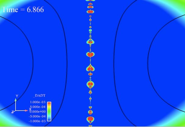
What is Automatic Differentiation (AD)?

• Technique to compute analytic
  derivatives without hand-coding the
  derivative computation

• How does it work -- freshman calculus
   – Computations are composition
     of simple operations (+, *, sin(),       2.000   1.000
     etc…) with known derivatives
   – Derivatives computed line-by-            7.389   7.389
     line, combined via chain rule
                                              0.301   0.500
• Derivatives accurate as original
  computation                                 0.602   1.301
   – No finite-difference truncation          7.991   8.690
     errors
                                              0.991 -1.188
• Provides analytic derivatives without
  the time and effort of hand-coding
  them
Sacado: AD Tools for C++ Codes

• Several modes of Automatic Differentiation
  –   Forward
  –   Reverse
  –   Univariate Taylor series
  –   Modes can be nested for various forms of         http://trilinos.sandia.gov
      higher derivatives
• Sacado uses operator overloading-based
  approach for C++ codes
  – Phipps, Gay (SNL ASC)
  – Sacado provides C++ data type for each AD
    mode
  – Replace scalar type (e.g., double) with template
    parameter
  – Instantiate template code on various Sacado AD
    types
  – Mathematical operations replaced by
    overloaded versions
  – Expression templates to reduce overhead
Our AD Tools Perform Extremely Well
(%"!#
!"#$%&"'()%"*+",$'(-&./(0/*",%/(1$(2"'34#$3/3(
($"!#
(!"!#
)*+,+-./#0.1.23#456#
'"!#
789#0.1.23#456#
&"!#
03:*18#;*.-.?3-#
%"!#
@.-2A13282#
$"!#
!"!#
!# $!# %!# &!# '!# (!!# ($!# (%!#
-$1"*(5/67//84$94:7//3$.(;/7()*/./'1(
• Simple set of representative PDEs
– Total degrees-of-freedom = number of nodes x number of PDEs for
each element
• Operator overloading overhead is nearly zero
• 2x cost relative to hand-coded, optimized Jacobian (very problem
dependent)AD to TBGP
• Benefits of templating
– Developers only develop, maintain, test one templated code base
– Developers don’t have to worry about what the scalar type really is
– Easy to incorporate new scalar types
• Templates provide a deep interface into code
– Can use this interface for more than derivatives
– Any calculation that can be implemented in an operation-by-operation
fashion will work
• We call this extension Template-Based Generic Programming (TBGP)
– Extended precision
• Shadow double
– Floating point counts
– Logical sparsity
– Uncertainty propagation
• Intrusive stochastic Galerkin/polynomial chaos
• Simultaneous ensemble propagation
– 2 papers under revision to Jou. Sci. Prog.Sandia Agile Components Strategy
• Create, use, and improve a common base of software
components
– Component = modular, independent yet interoperable
software
• Libraries, interfaces, software quality tools, demo applications
– Leverage software base for new efforts
– Use new efforts to improve software base
– Path to impact for basic research (e.g., ASCR)
• Large effort encapsulating much of SNL CIS R&D
– Driven by Andy Salinger
• Foundation for new simulation code efforts
– E.g., Drekar for CASL (Pawlowski, Cyr, Shadid, Smith)Analysis Tools
(black-box) The Components Effort is Large (~100 modular pieces)
Optimization Utilities
Composite Physics
UQ (sampling) Input File Parser
Parameter Studies MultiPhysics Coupling Data-Centric Algs
System Models Parameter List
V&V, Calibration Memory Management Graph Algorithms
OUU, Reliability System UQ SVDs
I/O Management
Analysis Tools Mesh Tools Communicators Map-Reduce
(embedded) Linear Programming
Mesh I/O
Nonlinear Solver PostProcessing Network Models
Inline Meshing
Time Integration Visualization
Partitioning
Continuation Verification
Load Balancing
Sensitivity Analysis Model Reduction
Adaptivity
Stability Analysis Remeshing Mesh Database
Constrained Solves Software Quality
Grid Transfers Mesh Database
Optimization Quality Improvement Geometry Database Version Control
UQ Solver DOF map Solution Database Regression Testing
Build System
Linear Algebra Local Fill Backups
Data Structures Discretizations
Verification Tests
Iterative Solvers Discretization Library Physics Fill Mailing Lists
Direct Solvers Field Manager Element Level Fill Unit Testing
Eigen Solver Material Models
Derivative Tools Bug Tracking
Preconditioners
Sensitivities Objective Function Performance Testing
Matrix Partitioning
Derivatives Constraints Code Coverage
Architecture- Error Estimates Porting
Dependent Kernels Adjoints
UQ / PCE MMS Source Terms Web Pages
Multi-Core Propagation Release Process
AcceleratorsTemplating is a Key Component Software Design
Principal
• C++ templating is a powerful method of abstraction
– STL containers
– Boost MPL
– Trilinos Kokkos node API
• Templating components on the scalar type provides API
to support embedded algorithms
– Developers focus on component implementation
– Embedded quantities are easily incorporated
– Scalable to many embedded techniquesTemplated Components Orthogonalize Physics
and Embedded Algorithm R&D
Application Interface Field Manager
Nonlinear solver Scatter (Extract) DOF Manager
computeResidual()
Optimization computeJacobian()
PDE Terms
Discretization
computeTangent()
Properties
UQ Cell Topology
computeHessian()
Source Terms Mesh
computeAdjoint()
Error estimation FE Interpolation MDArray
computePCE() Compute Derivs
Stability Analysis computeResponse() Get Coordinates
… Gather (Seed)
… DOF Manager
Legend: Template Specializations for
Global Data Structures Seed and Extract phases:
Application
component/library Local Data Structures Residual Hessian
Jacobian Adjoint
Embedded Analysis Generic Template Type
component/library used for Compute Phase Tangent PCEApproach Supports Complex Physics
Development
Albany/QCAD – Quantum Device Modeling
Albany/LCM – Thermo-Elasto-Plasticity – R. Muller et al
– J. Ostein et al
Charon/MHD – Magnetic Island Coalescence Drekar/CASL – Thermal-Hydraulics
– Shadid, Pawlowski, Cyr – Pawlowski, Shadid, Smith, CyrEmbedded Algorithms R&D using TBGP
Polynomial Chaos Expansions (PCE)
• Steady-state finite dimensional model problem:
         Find u(ξ) such that f (u, ξ) = 0, ξ : Ω → Γ ⊂ RM , density ρ

• (Global) Polynomial Chaos approximation:
                                 P
                                 �                                �
        u(ξ) ≈ û(ξ) =                 ui Ψi (ξ),   �Ψi Ψj � ≡            Ψi (x)Ψj (x)ρ(x)dx = δij �Ψ2i �
                                 i=0                                  Γ

• Non-intrusive polynomial chaos (NIPC, NISP):
                         �                                            Q
                                                                      �
                  1                                           1
         ui =                    û(x)Ψi (x)ρ(x)dx ≈                        wk ūk Ψi (xk ), f (ūk , xk ) = 0
                �Ψ2i �       Γ                              �Ψ2i �    k=0
• Regression PCE:                      P
                                       �
      û(xk ) = ūk =⇒                       ui Ψi (xk ) = ūk , f (ūk , xk ) = 0, k = 0, . . . , Q
                                       i=0
• Reduce number of samples by adding derivatives
  – Mike Eldred (SNL ASC)
                                   P
                                   �
                                          ui Ψi (xk ) = ūk , k = 0, . . . , Q
                                   i=0
                                 P
                                 �          ∂Ψi             ∂ ūk
                                       ui         (xk ) =            , k = 0, . . . , Q
                                 i=0
                                             ∂x             ∂xk
Computing Accurate Gradients Efficiently
in PDE Simulations
• Steady-state sensitivities
– Forward:
f (u∗ , p) = 0,
s∗ = g(u∗ , p) =⇒
� �−1
ds∗ ∂g ∗ ∂f ∗ ∂f ∗ ∂g ∗
=− (u , p) (u , p) (u , p) + (u , p)
dp ∂u ∂u ∂p ∂p
– Adjoint :
� �T � �T � �−T � �T � �T
ds∗ ∂f ∂f ∂g ∂g
=− (u∗ , p) (u∗ , p) (u∗ , p) + (u∗ , p)
dp ∂p ∂u ∂u ∂p
– Single forward/transpose solve for each parameter/response
– Accuracy determined by accuracy of partials, solution to linear systems
• Transient sensitivities:
– Forward:
f (u̇, u, p) = 0,
∂f ∂ u̇ ∂f ∂u ∂f
+ + =0
∂ u̇ ∂p ∂u ∂p ∂p
– Transient adjoint sensitivities are possible, but much harderSmall Model Problem
• 2-D incompressible fluid flow past a cylinder
– Albany code -- stabilized Galerkin FEM
• SUPG, PSPG
– GMRES with RILU(2) preconditioning (Belos, Ifpack)
– Uncertain viscosity fieldComparisons on Model Problem
Solver Reuse for Sampling-based
Approaches
• Sampling method can be viewed as a block-diagonal
nonlinear system:
∂f1
f1 (u1 , x1 ) = 0 ∂u1 ∆u1 f1
.
..
=⇒ .. . = −
..
. . . .
∂fN
fN (uN , xN ) = 0 ∂u
∆uN fN
N
• Leverage reuse
– Preconditioner
– Krylov basis1,2
• Compute multiple residual/Jacobian samples
simultaneously
– Multi-point TBGP scalar type
a = {a1 , . . . , aN }, b = {b1 , . . . , bN }, c = a×b = {a1 ×b1 , . . . , aN ×bN }
– Improved vectorization, data locality
1C.Jin, X-C. Cai, and C. Li, Parallel Domain Decomposition Methods for Stochastic Elliptic Equations, SIAM Journal on
Scientific Computing, Vol. 29, Issue 5, pp. 2069—2114, 2007.
2Michael
L. Parks, Eric de Sturler, Greg Mackey, Duane Johnson, and Spandan Maiti, Recycling Krylov Subspaces for
Sequences of Linear Systems, SIAM Journal on Scientific Computing, 28(5), pp. 1651-1674, 2006Multi-point Sampling of Model Problem
• Only real improvement is
reusing preconditioner
• Recycling benefits can be
had just by recycling
between Newton stepsEmbedded Stochastic Galerkin UQ Methods
• Steady-state stochastic problem (for simplicity):
Find u(ξ) such that f (u, ξ) = 0, ξ : Ω → Γ ⊂ RM , density ρ
• Stochastic Galerkin method (Ghanem and many, many others…):
�P �
1
û(ξ) = ui ψi (ξ) → Fi (u0 , . . . , uP ) = 2
f (û(y), y)ψi (y)ρ(y)dy = 0, i = 0, . . . , P
i=0
�ψ i � Γ
– Multivariate orthogonal basis of total order at most N – (generalized polynomial chaos)
• Method generates new coupled spatial-stochastic nonlinear problem (intrusive)
F0 u0
F1 u1 ∂F
:
0 = F (U ) = . , U = .
.. .. ∂U
FP uP
• Advantages: Stochastic sparsity
Spatial sparsity
– Many fewer stochastic degrees-of-freedom for comparable level of accuracy
• Challenges:
– Computing SG residual and Jacobian entries in large-scale, production simulation codes
– Solving resulting systems of equations efficiently, particularly for nonlinear problemsStokhos: Trilinos tools for embedded
stochastic Galerkin UQ methods
• Eric Phipps, Chris Miller, Habib Najm, Bert Debusschere,
Omar Knio
• Tools for describing SG discretization
– Stochastic bases, quadrature rules, etc…
• C++ operator overloading library for automatically evaluating
SG residuals and Jacobians
– Replace low-level scalar type with orthogonal polynomial
expansions
– Leverages Trilinos Sacado automatic differentiation library
P
� P
� P
� P
� �ψi ψj ψk �
a= ai ψi , b = bj ψj , c = ab ≈ ck ψk , c k = ai bj
i=0 j=0 k=0 i,j=0
�ψk2 �
• Tools forming and solving SG linear systems
– SG matrix operators
– Stochastic preconditioners
– Hooks to Trilinos parallel solvers and preconditioners
• Nonlinear SG application code interface
– Connect SG methods to nonlinear solvers, time integrators,
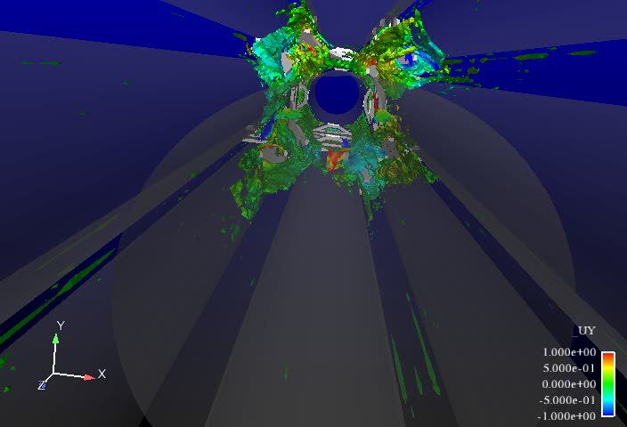
optimizers, …Embedded UQ in Drekar:
Multiphysics: Rod to Fluid Heat Transfer
• True multiphysics formulation: conjugate heat
transfer demonstrated in Drekar
• Embedded uncertainty quantification demonstration
run using TBGP concepts at the 1 year mark
• Agile components significantly decreases the time to
import cutting edge research into production
applications
Stochastic Galerkin UQ analysis propagating
uncertainty in the magnitude of the model fuel source term
and the average inflow velocity.Unique Embedded UQ R&D • Spatially adaptive UQ of a strongly convected field in Drekar – Eric Cyr – SNL LDRD – 2-D convection-diffusion with stochastically varying inlet angle – Intrusive stochastic Galerkin with spatially varying polynomial order • Possible only through embedded approaches
Comparison between linear and nonlinear PDEs
                Linear Problem                                       Nonlinear Problem
                                           3
        −∇ · (a(x, ξ)∇u) = 1, x ∈ [0, 1]                      −∇ · (a(x, ξ)∇u) = αu2 , x ∈ [0, 1]3
                  M �
                  �                                                       M �
                                                                          �
a(x, ξ) = µ + σ         λk fk (x)ξk , ξk ∼ U (−1, 1)    a(x, ξ) = µ + σ         λk fk (x)ξk , ξk ∼ U (−1, 1)
                  k=1                                                     k=1

 •   Albany FEM code
 •   AztecOO Krylov solver
 •   ML mean-preconditioner
 •   Stokhos approximate Gauss-Seidel stochastic preconditioner
Comparison between linear and nonlinear PDEs
• Difference in performance due to dramatically reduced
sparsity of the stochastic Galerkin operator
– Increased cost of matrix-vector products
Linear Problem
Nonlinear Problem
• On-going R&D
– Improved stochastic preconditioning
– Dimension reduction for SG Jacobian operator
– Multicore accelerationEmerging Architectures Motivate New Approaches
• UQ approaches usually implemented as an outer loop
– Repeated calls of deterministic solver
• Single-point forward simulations use very little available node
compute power (unstructured, implicit)
– 3-5% of peak FLOPS on multi-core CPUs (P. Lin, Charon, RedSky)
– 2-3% on contemporary GPUs (Bell & Garland, 2008)
• Emerging architectures leading to dramatically increased on-
node compute power
– Not likely to translate into commensurate improvement in forward
simulation
– Many simulations/solvers don’t contain enough fine-grained
parallelism
• Can this be remedied by inverting the outer UQ/inner solver
loop?
– Add new dimensions of parallelism through embedded approachesStructure of Galerkin Operator
• Operator traditionally organized with outer-stochastic, inner-spatial
structure
– Allows reuse of deterministic solver data structures and preconditioners
– Makes sense for sparse stochastic discretizations
P
� P
�
trad com
J = G k ⊗ Jk J = Jk ⊗ G k
k=0 k=0
Stochastic sparsity
Spatial sparsity
Spatial sparsity
Stochastic sparsity
• For nonlinear problems, makes sense to commute this layout to outer-
spatial, inner-stochastic
– Leverage emerging architectures to handle denser stochastic blocks
– Phipps, Edwards, Hu (SNL LDRD)SG Mat-Vec Floating-point Rate
="?:50@:9:"" "6>?"@$!A!"
AG" -0FG;0H73F"
HI>6J>G"AKB(F" '!" IJF5KFG"BMultiphysics Embedded UQ • SNL – Phipps, Constantine, Eldred, Pawlowski, Red-Horse, Schmidt, Wildey • USC – Ghanem, Arnst, Tipireddy
Stochastic Coupled Nonlinear Systems
• Shared-domain multi-physics coupling
   – Equations coupled at each point in domain
            L1 (u1 (x), u2 (x), ξ1 ) = 0
            L2 (u1 (x), u2 (x), ξ2 ) = 0

• Interfacial multi-physics coupling
   – Equations are coupled through boundaries
L1 (u1 (x), v2 (x2 ), ξ1 ) = 0,   v2 (x2 ) = G2 (u2 (x2 )),   x2 ∈ Γ2
L2 (v1 (x1 ), u2 (x), ξ2 ) = 0,   v1 (x1 ) = G1 (u1 (x1 )),   x1 ∈ Γ1

• Network coupling
   – Equations are coupled through a set of scalars
            L1 (u1 (x), v2 , ξ1 ) = 0,   v2 = G2 (u2 )
            L2 (v1 , u2 (x), ξ2 ) = 0,   v1 = G1 (u1 )
Curse of Dimensionality
• All three forms can be written after discretization
f1 (u1 , v2 , ξ1 ) = 0, u1 ∈ Rn1 , v2 = g2 (u2 ) ∈ Rm2 , f1 : Rn1 +m2 +M1 → Rn1
f2 (v1 , u2 , ξ2 ) = 0, u2 ∈ Rn2 , v1 = g1 (u1 ) ∈ Rm1 , f2 : Rm1 +n2 +M2 → Rn2
• Because system is coupled, each component must compute approximation over
full stochastic space:
û1 (ξ1 , ξ2 ) = û1 (v̂2 (ξ1 , ξ2 ), ξ1 )
– For segregated methods, requires solving sub-problems of larger dimensionality
– Adding more components, or more sources of uncertainty in other components, increases
cost of each sub-problem
• Mitigate curse of dimensionality by defining new random variables
P
� P̃1
�
û1 (ξ1 , ξ2 ) = u1,j Ψj (ξ1 , ξ2 ) −→ ũ1 (η2 , ξ1 ) = ũ1,j Φj (η2 , ξ1 ), η2 = v̂2 (ξ1 , ξ2 )
j=0 j=0
– Size of each UQ problem now number of uncertain variables + number of interface
variables
– Challenges: computing new orthogonal polynomials, associated quadrature rulesStochastic Dimension Reduction
• Consider simplified problem of composite functions
h(x) = g(y), y = f (x), f : Γ ⊂ RM → RL , g : f (Γ) → RS , L � M
Q
�
• with discrete inner product (f1 , f2 ) = wk f1 (x(k) )f2 (x(k) )
k=0
P
�
• We wish to approximate ĥ(x) = hi Ψi (x), hi = (h, Ψi ), V = span{Ψi }
i=0
• Conceptual basis for dimension reduction:
– Compute subspace W given by span of monomials
� in y, projected onto �
V
P
� � kL
�
y = f (x) = (y1 , . . . , yL ), W = span y1k1 . . . yL , Ψi Ψi ⊂V
i=0
– Compute orthogonormal basis for this subspace
span{Φi : i = 0, . . . , P̃ } = W, (Φi , Φj ) = δij , P̃ +1 = dim(W ), P̃ � P
– Compute reduced quadrature rule by requiring exactness on this space
Q̃
�
w̃l Φi (x(kl ) )Φj (x(kl ) ) = δij , Q̃ � Q
l=0
– Compute reduced projection
P̃
� Q̃
�
h̃(x) = h̃i Φi (x), h̃i = w̃l g(y (kl ) )Φi (y (kl ) ), y (kl ) = f (x(kl ) )
i=0 l=0
– Compute final transformation back to original basis
P
� P̃
�
h̄(x) = h̄i Ψi (x), h̄i = h̃j αij , αij = (Ψi , Φj )
i=0 j=0Devil is in the Details
• Computing W, orthogonal basis accurately is challenging
– Gram-Schmidt QR
• Variety of approaches for reduced quadrature
– Least-squares
– Linear program (arXiv: 1112.4772)
• In 1-D (L = 1) this is much easier
– Discretized Stieltjes = Lanczos (arXiv 1110.0058)
• Alternative approach
– Apply Lanczos approach to each component of y
• 1-D orthogonal polynomials, Gauss rules
– Total order tensor product polynomials, sparse grid quadrature
• This spans W, but is not an orthogonal basis!
– Project onto this basis using this quadrature rule/inner product
– Project onto original basis, using above as a surrogate
• Relying on point-wise convergence w.r.t. wrong inner product/measure
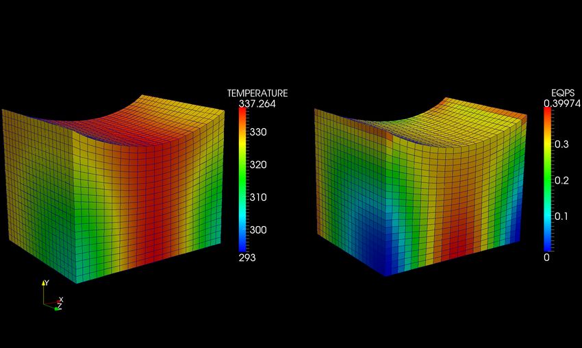
• This can fail catastrophicallyCoupled neutron-transport and heat transfer
demonstration
• 2-D “slab reactor” (H. Stripling):
�
1
Q− Φ(x)Σf (T̄ )Ef dx = 0 s.t. − ∇ · (D(T̄ )∇Φ(x)) + (Σa (T̄ ) − νΣf (T̄ ))Φ(x) = S(x, ξ1 ),
L2 D
�
1
T̄ − 2 T (x)dx = 0 s.t. − ∇ · (k(x, ξ2 )∇T (x)) = Q,
L D
�
2 T¯0 1
x ∈ D = [0, L] , Σ(T̄ ) = Σ(T0 ) , D=
T̄ 3(Σa + Σs )
M �
� M
� √
S(x, ξ1 ) = S0 (x) + σS λi ai (x)ξ1,i , k(x, ξ2 ) = k0 (x) + σk µi bi (x)ξ2,i ,
i=0 i=0
ξ1,i , ξ2,i Uniform on (−1, 1)
• 2-component network system, nonlinear elimination coupling
– Non-intrusive: Sparse-grid quadrature provided through Dakota on space of size 2*M
• Dimension reduction:
– Tensor-product Lanczos variant of approach outlined previously
– Intrusive (stochastic Galerkin) at 2x2 network level, non-intrusive for each component
– Each component UQ problem of size M+1Results
Dimension Reduction in Shared-Domain/
              Interfacial Coupling
• Approaches rely on small dimensional interfaces between physics
  – Network coupling – built into the model
  – Shared-domain/interfacial – transfer between physics may live on
    small dimensional manifold
     • Use KL to parameterize this (arXiv: 1112.4761)
                           40                                                                                  4
                                                                                                        x 10
                                                                                                   2

                           30
                                                                                                  1.5
          Eigenvalue [ï]

                                                                                Eigenvalue [K2]
                           20
                                                                                                   1

                           10
                                                                                                  0.5

                            0
                             0        2          4               6     8   10                      0
                                                     Index [ï]                                      0              2          4               6     8   10
                                                                                                                                  Index [ï]

                                 !                                                                      !

                                "#!                                                                "#!
           d"&'ï(

                                                                                 d"&'ï(

                                 $                                                                      $

                           ï"#!                                                                   ï"#!

                                ï!                                                                  ï!
                                 ï!       ï"#!             $         "#!    !                        ï!                ï"#!            $          "#!    !
                                                        d%&'ï(                                                                       d%&'ï(
Concluding Remarks • Looked at a variety of embedded UQ algorithms leverage structure – Simulation structure – Architecture structure • An approach for incorporating them in large-scale codes – Template-based generic programming – Agile components • Powerful vehicle for investigating embedded algorithms with path to impact important applications
Nonlinear Elimination for
                     Network Coupled Systems

                                    Component 1
          v2 = G1 (v1 , p1 ) = g1 (u1 (v1 ), p1 ) s.t. f1 (u1 , v1 , p1 ) = 0
v1                                                                                       v2
                                    Component 2
          v1 = G2 (v2 , p2 ) = g2 (u2 (v2 ), p2 ) s.t. f2 (u2 , v2 , p2 ) = 0

                              Nonlinear elimination
         Equations                                      Newton Step
                                    �                         ��    �    �                   �
     v2 − G1 (v1 , p1 ) = 0          −dG1 /dv1      1           ∆v1       v2 − G1 (v1 , p1 )
                                                                      =−
     v1 − G2 (v2 , p2 ) = 0             1        −dG2 /dv2      ∆v2       v1 − G2 (v2 , p2 )
                                                                 �    �
                                                 dGi         ∂gi ∂fi −1 ∂fi
                                                        =−
                                                  dvi        ∂ui   ∂ui     ∂vi
You can also read