Formation of Halos and their Abundance in the Universe
←
→
Page content transcription
If your browser does not render page correctly, please read the page content below
Formation of Halos and their
Abundance in the Universe
The growth of density perturbations eventually leads to non-
linear growth and collapse, forming halos in the Universe. The
abundance and redshift evolution of the halos is sensitive to a
range of cosmological properties, including the expansion
history, the growth rate of structure and the nature of the
underlying density field.
Overview
 n    Non-linear dynamics of a perturbation

 n    Press Schechter model for abundance of collapsed halos

 n    Application to Galaxy Cluster Surveys
        n       What are the ingredients of a real world survey?
        n       Review of recent, ongoing and future projects
                 n   Studies of Dark Energy
                 n   Studies of Non-Gaussianity
                 n   Tests of the L-CDM paradigm
                 n   Consistency tests for General Relativity- the growth rate of structure

 4. June 2021                       Cosmology and Large Scale Structure - Mohr - Lecture 5    2
Spherical Collapse Model
n     An analytical connection between linear and non-linear collapse exists
      in the so-called spherical collapse model

n     Consider a spherical tophat overdensity in an expanding universe with
      radius R and initial overdensity d

n     Solutions parallel those for the evolution of the scale factor and time in
      a closed, matter dominated homogeneous and isotropic universe
                                 a (t )                   Ωo
                                          = (1− cosθ )
                                 a ( to )              2 (Ωo −1)
                                                                   Ωo
                                   H ot = (θ − sin θ )                     3
                                                             2 (Ωo −1)         2

n     Where q is a development angle runs from 0 to 2p
                                                                                     Discussion follows Liddle and Lyth
    4. June 2021            Cosmology and Large Scale Structure - Mohr - Lecture 5                               3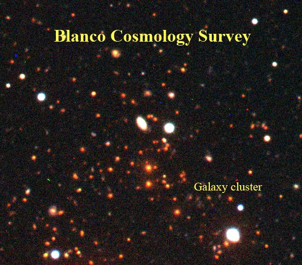
Linearized Scale Factor
n     By examining those expressions at the maximum expansion amax and
      time of maximum expansion tmax we can write
                                    a (t ) 1
                                          = (1− cosθ )
                                    amax 2
                                       t       1
                                           =     (θ − sinθ )
                                    tmax       π
n     To study the linear regime of these solutions we can use the small
      parameter expansions of both expressions
                       a (t ) θ 2 θ 4                    t      1 #θ 3 θ 5 &
                             ≅ −      and                      ≅ % −       (
                       amax 4 48                        tmax    π $ 6 120 '
n     Combining these one can solve for a linearized scale factor alin
                                            3)              3,
                                                    2                               2
                        alin (t ) 1 "   t % +   1 "    t % .
                                 ≅ $ 6π    ' 1− $ 6π      '
                         amax     4 # tmax & +* 20 # tmax & .-
    4. June 2021           Cosmology and Large Scale Structure - Mohr - Lecture 5       4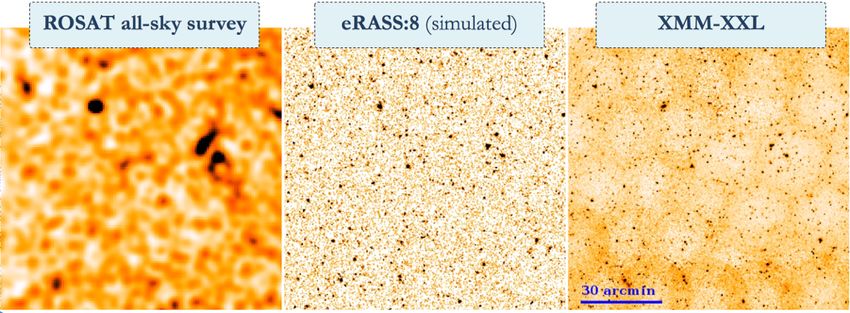
3)              3,
                                                                                   2                2
                                                                 alin (t ) 1 "   t % +   1 "    t % .
                                                                          ≅ $ 6π    ' 1− $ 6π      '
Linear Evolution Cont                                             amax     4 # tmax & +* 20 # tmax & .-

 n    Ignoring the bracketed expression we see a~t2/3, which we recognize
      as the expression for the background evolution

 n    The full expression is for the evolving perturbation

 n    Consider turnaround (a=amax) and the perturbation overdensity
                                                       3
                                                     aback
                                         1+ δlin =      3
                                                      alin
 n    Substituting in the preceeding expressions gives       2

                                               3!    t $
                                                          3

                                        δlin = # 6π     &
                                              20 " tmax %
 n    So at turnaround, t=tmax, the linear density contrast is
                                 turn      3      2
                             δ  lin     =    (6π ) 3 ≈ 1.06
                                          20
 4. June 2021             Cosmology and Large Scale Structure - Mohr - Lecture 5                        5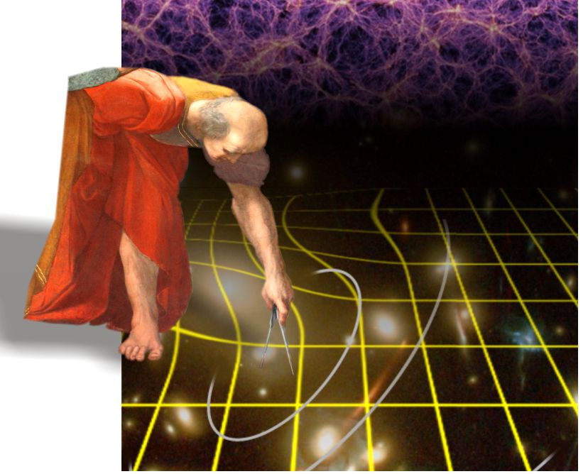
Collapse Overdensity
n     After turnaround the collapse proceeds symmetrically to the
      expansion phase, and so at t=2*tmax the perturbation has collapsed
                                      coll         3       2
                                    δlin   =         (12π ) 3 ≈ 1.686
                                                  20
n     So the linear density contrast of d~1.7 corresponds to a threshold
      density at which the underlying density perturbation would have
      collapsed and formed a halo
n     The actual non-linear density contrast at turnaround is    2

                                  1+ δ   turn      a3
                                                  = back =
                                                           (6π ) ≈ 5.55
                                         nonlin     3
                                                   amax      43
n     If we assume that the collapsing object virializes at half the radius, its
      density will have gone up by a factor of 8. Relative to the background
      density the nonlinear overdensity of the collapsed halo is
                                                 vir
                                             1+ δnonlin ≈ 178
n     N-body simulations confirm that the region of the halo with an
      overdensity of ~200 corresponds to the virialized portion of the halo
    4. June 2021            Cosmology and Large Scale Structure - Mohr - Lecture 5   6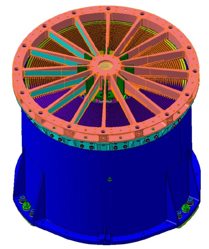
Connecting linear growth to halo abundance
evolution: The Press-Schechter Mass Function
n     Consider the cosmic density field filtered on a mass scale M
        n   Gaussian distribution of over/under density with width s
        n   Over cosmic time perturbations grow and s increases

                                                      collapsed

                                                                                 collapsed
                                                 dc                           dc

                              Gaussian Distributed Perturbations on Scale M

n     Consider the number density of collapsed (highly nonlinear) objects on a mass
      scale M
        n   Assume that density perturbations have collapsed by the time their linearly evolved
            overdensity exceeds some critical value dc
        n   Abundance (number density) of collapsed objects with mass M is then proportional
            to an integral over the tail of a Gaussian distribution
                                                            ∞
                                    ρ              1
                            n(M,z) = b
                                    M
                                                            ∫
                                                2πσ ( M,z) δ c
                                                               dδ exp           {     2σ
                                                                                             −δ
                                                                                             2
                                                                                                  2

                                                                                                 ( M ,z)   }
    4. June 2021                  Cosmology and Large Scale Structure - Mohr - Lecture 5                       7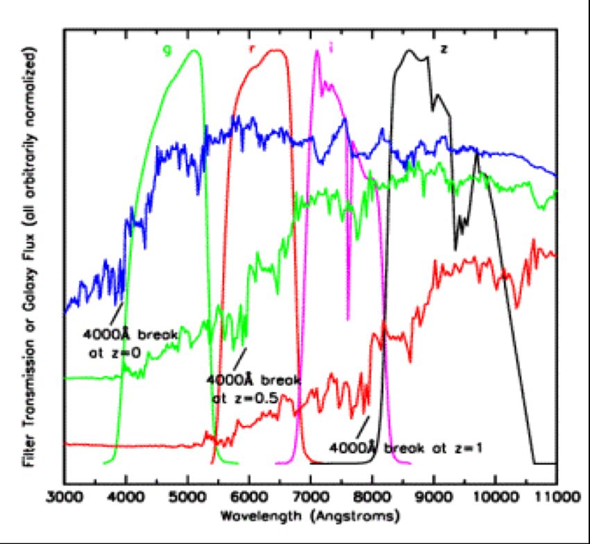
Halo Abundance
    n   Cluster mass function dn(M,z)/dM depends on
        mean matter density and amplitude of density
        fluctuations
                  σ 2 (M ) =    1
                               2π 2
                                         3
                                      ∫ d k P(k) W (k, M )     2

                  where W (k, M ) is the Fourier transform of the spherical tophat

         n   Vintage Press-Schechter formalism

               dn               ρ b dσ ( M , z)    δc          ' −δ 2 *
                              2
                  (M , z) = − π                             exp( 2 c +
               dM               M     dM        σ 2 (M , z)    ) 2σ ( M ,z) ,

         n   Modern numerical simulations: Jenkins et al 2001
               dn                  ρ b dσ (M , z) 1    %                     3.8 (
                  (M , z) = −0.315                  exp&− 0.61− log(D zσ M )     )
               dM                  M     dM      σ     '                         *

4. June 2021                                 Cosmology and Large Scale Structure - Mohr - Lecture 5   8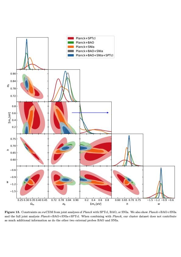
Mass Function Now Studied with Numerical
Simulations of Structure Formation
n      Extracted from sixteen billion
       particle dark matter simulation.
                                                                                     Warren et al ‘06

n      Halos are defined using a
       friends of friends algorithm

n      Halo masses are assigned
       using mass within spherical
       overdensity

    4. June 2021            Cosmology and Large Scale Structure - Mohr - Lecture 5                      9
Cosmological Dependence
   n     Direct tests using N-body simulations in good agreement with simple
         theoretical models (Sheth and Tormen 1999) over 5 orders of
         magnitude in mass

   n     Halo abundance is sensitive to cosmology through
           n   Mean background density
                                                                                                   Growth function sensitive
           n   The power spectrum of density fluctuations                                           to expansion history of
           n   Linear growth rate of density perturbations                                                 Universe.

                                                                           δ˙˙ + 2 a˙ δ˙ = 4 πGρ oδ
   n     The fitting functions have been tested over a wide range of LCDM          a
         cosmologies and have been shown to be accurate at better than 10%                δρ           a˙
         level                                                             where    δ   ≡      and H =
                                                                                          ρo           a

   n     Direct simulation required if better precision needed- “emulators”
         becoming common now

                dn                 ρ dσ (M , z) 1                         3.8 (
                   (M , z) = −0.315 b             exp%
                                                     & − 0.61− log ( z M ) )*
                                                                    D σ
                dM                 M   dM      σ     '
4. June 2021                              Cosmology and Large Scale Structure - Mohr - Lecture 5                         10
Baryon Impacts
Bocquet+16
n Baryons correspond to
~15% of the matter, and so Hydro
complex physics that DMonly
≠m
impacts baryons (star Tinker08
input
formation, radiative cooling,
magnetic fields, cosmic ray 0.8125
support, AGN feedback) can 0.8100
æ8
also impact the mass 0.8075
function 0.8050
æ8 (≠m /0.27)0.3
0.810
0.807
n The baryon impact is 0.804
comparable to a shift (or 0.801
bias) in the cosmological 0.260 0.265 0.270 0.804 0.808 0.812 0.800 0.805 0.810
parameters and must ≠m æ8 æ8 (≠m /0.27)0.3
therefore be accounted for
4. June 2021 Cosmology and Large Scale Structure - Mohr - Lecture 5 11Galaxy Clusters as Probes of Density
Perturbations and their Evolution
= Galaxy clusters are excellent tracers of structure formation
= A galaxy cluster survey is a powerful probe of the cosmic acceleration
= As we probe to higher redshift we see clusters disappear, and the exact rate at which
they disappear is (exponentially) sensitive to the growth rate of density perturbations
Evrard et al 2002
4. June 2021 Cosmology and Large Scale Structure - Mohr - Lecture 5 12Cluster Surveys as a Test of Cosmology
n A real world application requires a population of objects for
which the masses can be estimated accurately
n Galaxy clusters are one such population
n Here we review the ingredients of a cluster survey, highlight
some recent results, an ongoing project and briefly review some
future projects
4. June 2021 Cosmology and Large Scale Structure - Mohr - Lecture 5 13What Are Galaxy Clusters?
Galaxy clusters are the most massive, !"#$!"%&!
SPT-CLJ0205
!"%$!"&%" !"!'!"&%( !"()!"&!!
!
collapsed structures in the universe. They #8(!*92:;
%##
567/012324
#"!*+,-
contain galaxies, hot ionized gas (107-8K) #
and dark matter.
! ! !%##
$
#"!*+,-
./012324
In typical structure formation scenarios, low #
mass clusters emerge in significant ! ! !$
"
numbers at z~2-3
./012324
'"*+,-
#
Clusters are good probes, because they are ! ! !"
"
Data and
data andfolded
folded model model
(("*+,-
massive and “easy” to detect through
./012324
#
counts s keV[s‐1.keV‐1]
their:
83
z~1.38
! !"
0.015
kT~8.5keV
82
• X-ray emission (Bremsstrahlung)
−1
normalizedcounts
Statistic: L−statistic
−1
81
• Sunyaev-Zel’dovich Effect (Inverse Compton)
0.01
�2
Normalized
• Light from galaxies (Black Body)
80
5×10⁻³
79
Note: Galaxy clusters are NOT the most massive bound structures in the Universe.
Can you think of a more massive bound structure? 0 2
Energy (keV)
1.25
Energy [keV] kanderss 26−Jul−2011 10:07
4. June 2021 Cosmology and Large Scale Structure - Mohr - Lecture 5 14Galaxy Cluster Redshift Distribution
and Cosmology
n Cluster redshift distribution dN(z)/dz/dW
cluster mass function
abundance of detectable clusters
dN(z) dV 2 ∞ dn ( M,z)
= n (z) = c 2
d (1+ z) ∫ dM
dzdΩ dz dΩ H ( )
z A dM
m ( z)
lim
volume element
Minimum mass of detectable cluster
(typically function of redshift)
€
Critical components: Volume element
Mass function
Limiting mass
4. June 2021 Cosmology and Large Scale Structure - Mohr - Lecture 5 15Galaxy Cluster Surveys and Survey Yields
Cluster surveys probe (1) volume-redshift relation, (2) abundance evolution, (3) structural evolution
SZ-Array Survey
Surveys Constrain:
• Cluster surface density
• LogN-LogS
• Angular distribution
• Redshift distribution
• (Mass) function
4. June 2021 Cosmology and Large Scale Structure - Mohr - Lecture 5 16The Volume-redshift Relation
Volume Element
n Volume-Redshift Test
n Count non-evolving tracers
n measure volume
dV 2 2
= c d A (1 + z)
dzdΩ H ( z)
d A (1 + z) is proper distance
H (z) = H o E(z ) is the Hubble parameter
n But cluster density evolves as well
4. June 2021 Cosmology and Large Scale Structure - Mohr - Lecture 5 17Abundance Evolution and Cosmology
n Normalize locally Comoving Abundance
n Measure the abundance of galaxy
clusters
n High redshift abundance sensitive
to the growth rate of structures
4. June 2021 Cosmology and Large Scale Structure - Mohr - Lecture 5 18Importance of the Survey Detection Limit
Cluster redshift distribution dN(z)/dz/dW
∞
dN (z)
= Hc( z) d 2A (1 + z ) 2
dn( M,z ) Minimum mass of detectable cluster
dzdΩ ∫ dM dM
m lim
Mass Sensitivity
Limiting mass Mlim(z)
n Connecting cluster virial mass to observables is
critically important
n X-ray luminosity or emission weighted
temperature
n SZE luminosity
n Weak lensing shear amplitude
n Galaxy light / dynamical estimators
Total SZE flux from Cluster
−4 kν 2 σ T Tcmb 1 f ICM Mvir Te n
Stot =
m c4e d2 A
µe m p
4. June 2021 Cosmology and Large Scale Structure - Mohr - Lecture 5 19Clusters Have No Outer Surface
n Dark matter, ICM, and galaxy Galaxy Distribution in 89 Clusters
distributions all fall off with
distance from the cluster
center, but there’s no clear
signature of the edge of the
cluster
n There are preferred definitions
of cluster mass- we choose a
region which is a few hundred
times denser than the
background or critical density Lin, Mohr and Stanford 2004
motivated by spherical collapse
model but also from structure
formation simulations
4 3
M 200 = π R200 ∗ 200 ρcrit
3
4. June 2021 Cosmology and Large Scale Structure - Mohr - Lecture 5 20Cluster Mass Measurements
n There are three methods of measuring cluster masses directly:
n Assume hydrostatic equilibrium, use X-ray observations:
n Measure the temperature and density profiles using X-ray observations
n Infer the mass profile
n Assume virial equilibrium, use galaxy kinematics:
n Measure the velocities of a large number of galaxies within each cluster
n Relate the kinetic energy in the galaxies to the potential energy (mass)
n Use weak lensing (no equilibrium assumption needed)
n Map the gravitational lensing distortions due to the cluster lense
n Infer the mass profile – non-trivial, too
n All these methods are time and data intensive. In a cluster survey we rely on
inexpensive observables that serve as mass proxies:
n X-ray luminosity, SZE flux, number of galaxies
n Must calibrate the relation between observable and mass
n Mass-Observable relation
n Single cluster mass estimate must not be precise but must be unbiased/accurate
n WL mass constraints available for “all” clusters overlapping modern surveys like DES
4. June 2021 Cosmology and Large Scale Structure - Mohr - Lecture 5 21Mass-Observable Relation 24 A. Mantz et al.
Power-law relation between
0.5 1.0 1.5
0.5 1.0 1.5
n
mass and observable,
redshift evolution and
log luminosity
log luminosity
characterization of scatter
−0.5
−0.5
about the relation are all
important
−1.5
−1.5
n Minimum of 4 nuisance
parameters −1.0 −0.5 0.0
log mass
0.5 1.0 −1.0 −0.5 0.0
log mass
0.5 1.0
n Must match fidelity of 0.5 1.0 1.5
0.5 1.0 1.5
model to the dataset
log luminosity
log luminosity
n Selection effects critical
−0.5
−0.5
n Malmquist bias
Eddington bias
n
Mantz et al 2010
−1.5
−1.5
n Unbiased mass estimator −1.0 −0.5 0.0
log mass
0.5 1.0 −1.0 −0.5 0.0
log mass
0.5 1.0
critical Figure A1. Fictitious cluster luminosity–mass relations (red lines) and simulated data (crosses) intended to illustrate the effect of
4. June 2021 Cosmology
Malmquist and Large
and Eddington Scale
biases Structure
on the - Mohr data.
scaling relation - Lecture
In the5 top panels, clusters are distributed uniformly in22log-mass, whereas
in the bottom panels the distribution of log-masses is exponential. The left-hand panels reflect the true distribution of all clusters in mass
and luminosity, while the right-hand panels show only the simulated clusters with luminosities greater than a threshold value, indicatedCluster Survey Cosmology Requirements
n Accurate predictions for the
mass function and its evolution
within a range of cosmological Warren et al ‘05
models that one wishes to
study
n Comparing observed and
simulated mass function shape
and evolution requires: Dark Matter Halo Mass Function
n Well understood selection
n Ability to estimate mass
n Cluster redshift measurements
4. June 2021 Cosmology and Large Scale Structure - Mohr - Lecture 5 23Clean Cluster Selection Chandra Image of Zw3158
= In addition to accurate cluster masses,
the selection of the sample is also very
important
= Clusters can be selected in the optical, X-
ray or SZE
= None of these provide a clean selection
by mass, because the mass-observable
relations exhibit significant scatter
SZE
X-ray
= Currently the SZE selection provides the
cleanest selection
IΔT(R)
x (R) = 1 µe
∫ dl n
2
e (l,
(1+ z ) 4 2µ H∫ dl ne (l,
=4 π−2
σ T
R)
R)Λ(Te )
kB Te (l, R)
me c
Tcmb
4. June 2021 Cosmology and Large Scale Structure - Mohr - Lecture 5 24Cluster Selection Methods
n eROSITA
Cluster finding: SZE, X-ray and Optical Extragalactic sky
mm-wave Sky
Image credits: MPE, eRosita_D
In all cases, use cluster Red Sequence galaxies to estimate redshift
Wide-area census of galaxy clusters (105) and active galactic
4. June 2021 Cosmology and Large Scale Structure - Mohr - Lecture 5 25d N dn dV
d ln M dz M,z
=
d ln M M,z dz
⌦survey (M500c , z)
Poisson realisation of Mass Function, Tinker+08 Bulbul+18 Metallicity
(LX , TX ) Z = 0.3Z
Luminosity Temperature McDonald+16,
Cluster Selection Methods
Spectrum + ARF
n Cluster finding: SZE, X-ray and Optical
n Use cluster Red Sequence galaxiesintr. countredshift
rate ⌘
+ Poisson noise
to estimate
texp = 1.6ks
n Selection in observable implies meas. photon counts
mass selection, given n̂
a mass-
observable relation
n Typically power law
n Scatter in obs at fixed mass combines
intrinsic & measurement components X-ray photon count rate
n Cosmology dependence easily modeled
n Calibration through weak lensing,
dynamical constraints
!3
S. Grandis, HSC-eROSITA w., U of Tokyo, 12.XII.18
4. June 2021 Cosmology and Large Scale Structure - Mohr - Lecture 5 26Cluster Selection: Optical/IR
BGC versus Mass in Simulated Catalog
n Optical/IR Surveys
n Optical/IR signature only crudely related to Completeness f(M,z)
cluster mass- clean mass selection for SDSS-like Survey
impossible
n But see Rozo et al 2013- Richness-X-ray
relations (Micm and Lx) suggest 25%
intrinsic scatter in richness-mass. Saro et
al 2015 in agreement for richnesses of
clusters that are SZE selected
n Galaxies (even red ones) exist
everywhere, not just in clusters-
contamination an issue
Song et al 2009
n Completeness of red sequence methods
seems quite good
4. June 2021 Cosmology and Large Scale Structure - Mohr - Lecture 5Song et al 2012 27Cluster Selection: X-ray
n ROSAT experience:
n high completeness (~95%), low Chandra Image of Zw3158
contamination (~1%)
Reiprich & Böhringer 2002
n X-ray surveys
n X-ray luminosity tracks cluster mass
with ~45% scatter
n AGN can boost flux, leading to
contamination by low mass systems
n Unresolved clusters can be missed
unless there is complete multiband
optical imaging available to followup all
sources
n Low scatter mass estimate (Yx or Micm
at ~15% available for a subset)
4. June 2021 Cosmology and Large Scale Structure - Mohr - Lecture 5 28Sunyaev-Zel’dovich Effect
Ø SZ effect (SZE) is inverse Compton
scattering between low energy CMB
photons and high energy cluster
electrons
Ø SZE leads to a distortion of CMB
spectrum and therefore it is
redshift independent.
Ø SZE signal is a direct probe of total
thermal energy in cluster electron
population and hence a good proxy
for cluster mass.
Courtesy Leon
van Speybroeck
4. June 2021 Cosmology and Large Scale Structure - Mohr - Lecture 5 29Cluster Selection: SZE
n Unique signature in frequency Unique spectrum
and angle Unique angular scale
n Contamination just a function of S/N Need 10m telescope at 150GHz!
Need multiple frequencies!
n Clean mass selection
n SZE flux proportional to the total
thermal energy in the electron
population
n No cosmological dimming (indep of
z)
n Radio galaxies can bias flux, but
these very rare at high frequency
n SPT selection very clean- redshift
independent mass selection with 20% Simulations from M. White
mass scatter
4. June 2021 Cosmology and Large Scale Structure - Mohr - Lecture 5 30Contamination in Cluster Samples
n In SZE samples, contamination only through noise fluctuations
n To reasonable approx, only the cluster virial regions produce signal
n SPT cosmology sample starts with ~5% cont.
n Optical confirmation pushes toMeasuring Photometric Redshifts
• Measure relative flux in the
four filters griz: 50
ABELL1682 g-r vs.r
g-i vs. i
track the 4000 A break Song et al 2012 r-i vs. i
Nnet (=Ncluster-Nbkg)
r-z vs. z
40
i-z vs. z
• Estimate individual galaxy
30
redshifts with accuracy * at z~0.250
dz ~ 0.05-0.2 (more like 20
Gaussian fitting z~ 0.262
dz ~ 0.02 for clusters) ~ 0.033
10
• Use spectroscopic calibration 0
samples (>105) to control
-log(likelihood)
systematic uncertainties 15 Probability of being real cluster:
100.00 %
10
• Note: good detector
5
response in z band filter
0
needed to reach z>1
0.0 0.2 0.4 0.6 0.8 1.0 1.2
z
4. June 2021 Cosmology and Large Scale Structure - Mohr - Lecture 5 32Required Photometric Depths
= Photometry in the four bands Blanco Cosmology Survey Depths
must be deep enough to detect
galaxies of interest at the
redshift where the 4000A break
shifts out of the band
= g (z=0.35)
= r (z=0.7)
= i (z=1.0)
= z (z=1.4)
= For example, 10s galaxy limits
of (g,r,i,z=24.0,23.9,23.6,22.3) for
BCS survey (see figure)
= DES pushes deeper
4. June 2021 Cosmology and Large Scale Structure - Mohr - Lecture 5 33Historical Results
n Recent analyses of X-ray cluster samples using existing datasets have generally
been quite successful, but some problems have emerged with the optical samples
n SDSS and RCS were able to obtain interesting constraints on Wm and s8.
n RCS- 956 clusters over 72 deg2
n SDSS- 104 clusters over 7,400 deg2
Rozo et et
Gladders al al
2009
2007
4. June 2021 Cosmology and Large Scale Structure - Mohr - Lecture 5 34400 deg2 ROSAT Archival Sample
Vikhlinin et al 2009
n Analysis:
n 49 “local” + 37 z>0.35 clusters
0.6
Mass functions
BA
n 0, h =h0.72
ΩM = 0.25, ΩΛ = 0.75, = 0.72
100.7
O
n 12 clusters at z>0.55 require DE
−5 all
a
0.8 SN I
n Independent constraints in good
−6
100.9
agreement with WMAP+ cosmology
−3
0 Mpc
SN+BAO
n w constrained to 0.2(clus)/0.05(all) 1.0
+WMAP
N(>M), hw−3
10−7
WMA
1.1
P
1.2
10−8
1.3
clusters
101.4
−9
z = 0.025 − 0.25 +WMAP
1.5 z = 0.55 − 0.90
0.60 0.65 0.70 0.75 0.8015 0.85
1014 ⌦ 10
M500 , Xh −1 M"
4. June 2021 Cosmology and Large Scale Structure - Mohr - Lecture 5 35ROSAT All Sky Survey Sample
Mantz et al 2009
n Analysis:
n Mass function of full sample
n Constant fICM from 42 “relaxed” systems
n Mass-obs relation normalization freedom
allowed and constrained using 6 low z
clusters
n Independent constraints
n s8 = 0.82 (0.05)
n w=-1.01 (0.20)
n Combined constraints
n WMAP+SNe+BAO+Clusters+fICM:
n s8 = 0.79 (0.03)
n w=-0.96 (0.06)
n DETF FOM =15.5 (~2x improvement)
n wo=-0.93 (0.16), wa=-0.16 (+0.47,-0.73)
4. June 2021 Cosmology and Large Scale Structure - Mohr - Lecture 5 36South Pole Telescope (SPT)
¡ This is an ongoing large scale
cluster survey mission- finds
clusters over broad redshift
range using the SZE
¡ (Sub) millimeter wavelength
telescope:
§ 10 meter aperture
§ 1’ FWHM beam at 150 GHz
§ 20 micron RMS surface
§ 5 arcsec astrometry
¡ SZE Receiver:
§ 1 sq. deg FOV
§ Observe in 3 bands between 95-220 GHz
simultaneously
§ Sensitivity ~ 15-60 μK-arcmin
4. June 2021 Cosmology and Large Scale Structure - Mohr - Lecture 5 37SPT-SZ Survey Sky Coverage
n Survey 2008-2011
2491deg2 complete
n Data used to study CMB
anisotropy
n Select clusters through
Sunyaev-Zel’dovich Effect
Redshift independent
Tied closely to cluster mass
n Cluster candidates found:
657 at S/N>4.5
Now supplemented by SPTpol and SPT-3G
90GHz – 42 µK-armin 150GHz – 18 µK-armin 220GHz – 85 µK-armin
4. June 2021 Cosmology and Large Scale Structure - Mohr - Lecture 5 38Finding a Cluster in mm-wave Sky Maps
n Unique SZE signature helpsGalaxy
provideClusters!
pure sample
Galaxy Clusters!
n No redshift information – requires multi-l followup
111degree
degree
degree
150GHz
90
150 GHz
GHz
4. June 2021 Cosmology and Large Scale Structure - Mohr - Lecture 5 39First SZE Selected Galaxy Clusters
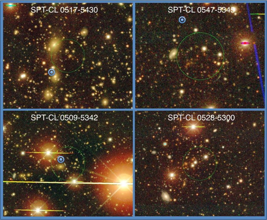
n July 14, 2008 initial SPT 0517 5430 0547 5345 0509 5342 0528 5300
candidate list was circulated 1.2 beam
200
Unfiltered
150 GHz
0
n Cross comparison to BCS 200
imaging immediately indicated: 8
150 GHz
Filtered
n Our SZE candidates were real! 0
n There was an ~arcminute scale
8
absolute pointing error in the SPT 6
maps
Filtered
95 GHz
0
n Initial demonstration sample 6
with BCS overlap and spanning 225 GHz
6
Filtered
full range of redshift published! 0
6
Staniszewski et al 2009
4. June 2021 Cosmology and Large Scale Structure - Mohr - Lecture 5 40SPT Optical Followup
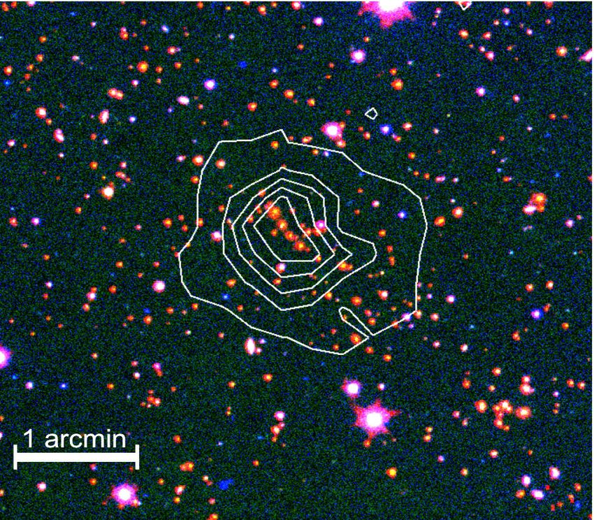
n We use multiband photometry to
get red sequence cluster Song et al 2012
redshifts
n Began with dedicated survey
Blanco Cosmology Survey –
60 nights/ 80 deg2/griz
n Now go cluster by cluster
n ~100 nights on the telescope so far
n Over 500 candidates imaged to date Characteristic scatter dz~0.018 for 0SPT-SZ Sample
Song+12 (720 deg2) , Bleem+15 (2500 deg2)
n 2500 deg2 sample
SPT-SZ 2500 deg2
n 516 at x>4.5 ROSAT-All sky
Planck-DR1
387 at x>5.0
70 ]
M500c [1014 MO• h-1
n ACT
10
Bleem+15
n High z subsample
n 36 at z>1
n Max zspec=1.47
1
Bayliss+13 0.0 0.5 1.0 1.5
n Max zphot=1.72 Bleem+15 Redshift
Strazzullo+18
n Clean sample with M500>3x10¹⁴ Mo to z~1.7
Now supplements by SPECS, SPTpol, SPT-3G…
4. June 2021 Cosmology and Large Scale Structure - Mohr - Lecture 5 42SPT Clusters: Contamination
n Negative noise peaks
Song et al 2012
can masquerade as
clusters
- Stay at high S/N!
n Optical confirmation
allows us to measure
the contamination
SPT-only selection produces >95% pure sample at S/N>5
SPT+optical followup produces ~100% pure sample at S/N>4.5
4. June 2021 Cosmology and Large Scale Structure - Mohr - Lecture 5 43Cluster Surveys Provide Multiple Handles on Dark Energy
Redshift Distribution Sensitive to DE
n Cluster surveys provide
Equation of State Parameter
n Redshift distribution
n Luminosity (mass) function
n Cluster power spectrum
n Direct mass calibration
n Each has different cosmological
dependence-- very rich dataset
10m South Pole Telescope
SZE Survey
dN(z) dV
= n ( z)
dzdΩ dz dΩ
Raising w at fixed WE:
n Decreases volume surveyed
n Decreases growth rate of density
perturbations
Volume effect Growth effect
4. June 2021 Cosmology and Large Scale Structure - Mohr - Lecture 5 44SPT Constraints on Dark Energy Bocquet+19
n 343 Clusters from 2500 deg2
n Mass calibration from gravitational
weak lensing of 32 clusters
n Cosmology limited by mass
uncertainties
n Cosmological constraints
n Clusters Only:
n Wm=0.276 (0.047)
n s8 = 0.781 (0.037)
n Planck+SNe+BAO+H0+SPT:
n w=-1.12 (0.21)
n Sum of neutrino masses 0.50 (0.24) eV
Largest available SPT sample (1000+) and DES weak lensing analysis coming soon!
4. June 2021 Cosmology and Large Scale Structure - Mohr - Lecture 5 45Non-Gaussianity and Halo Abundance
n In some models of inflation the 5.0
our fit to sims
resulting density perturbations have EPS
MVJ
nNG(z, M) / nG(z, M)
significant non-Gaussianity 4.0 f =+500
NL z=1
n For local non-Gaussianity parameter fNL the
perturbed gravitational potential takes the form z=0.5
3.0
(
Φ NG ( x ) = φ ( x ) + f NL φ 2 ( x ) − φ 2 )
2.0 z=0
n Positive fNL leads to an enhanced overdensity
relative to the corresponding Gaussian case
1.0
δ NG ≈ δ + 2 f NLφ p 1e+14 1e+15
-1
M (h Msun)
n Studies have revealed how this non- FIG. 6: Ratios of the NG to Gaussian mass functions as a functio
Gaussianity affects the mass function z = 1 (red). Points withDalal et aldenote
error bars 2008 results from our simul
dotted lines denote the EPS and MVJ fitting functions respectiv
n Positive fNL enhances the number of haloes in the significantly overestimate the effects of nongaussianity. (The disco
rare tails of the probability distribution at high is due to transition from a smaller simulation box to the larger on
mass and/or at high redshift
effects of nongaussianity as found by our simulations, at
4. June 2021 Cosmology and Large Scale Structure - Mohr
a level - Lecture
typically < 5100% although dependent upon
46 mass
∼
and redshift.SPT Constraints on Non-Gaussianity
n SPT constraints on non-Gaussianity
n fnl=-192+/-310, 20+/-450
(from full likelihood analysis including selection
function of SPT sample)
n For comparison, -10SZE Signature- A Solid Mass Indicator
n We have leveraged X-ray mass
indicators to calibrate our sample Andersson et al 2011
n Direct mass calibration underway
weak lensing and velocity dispersions
n High-z massive SPT clusters are
unique population
n M200>4x10¹⁴ Mo even at highest z
n Large solid angle survey (2500 deg2)
allows us to find very rare objects
n ~100 of these clusters over full survey
4. June 2021 Cosmology and Large Scale Structure - Mohr - Lecture 5 48Tests of LCMD and wCDM Paradigm
n The combination of CMB, SNe, BAO and Ho
constraints are already quite restrictive even without
z = 1.39 with an X-ray (TX ) mass of 7.7+4.4 14
the additional of galaxy cluster survey constraints
3.1 ⇥ 10 M .
These X-ray mass estimates are consistent with masses
obtained by other means such as weak lensing, and our
most conservative conclusions requiring 95% joint CL sig-
nificance in the full sky would not be greatly changed by
n Mortonson and collaborators explored this available
using alternate mass proxies.
parameter space in the standard, LCMD and
For a more aggressive interpretation of the data, one
can estimate the e↵ective fsky values for these measure-
wCDM models ments. They are somewhat subjective in that the clusters
are the most massive ones found in all high z Sunyaev-
n Flat geometry
Zel’dovich (SZ) and X-ray surveys respectively. The first
release of the South Pole Telescope (SPT) SZ cluster
n Gaussian density perturbations
survey covered 178 deg2 , whereas the Atacama Cosmol-
ogy Telescope SZ survey covered 455 deg2 [43] of which
n General relativity
⇠ 50 deg2 overlap with the first-release SPT fields. On
2
n Dark energythewith
otherequation of state
hand X-ray surveys paramsome
have covered w 283 deg
for 1.0 < z < 2.2 [12]. We therefore plot these clusters
in Fig. 4 (lower panel) against an exclusion curve for
95% joint CL at 300 deg2 , using h = 0.70 as assumed in
n They determined regions in mass and redshift
Refs. [41, 42] to convert the masses to units of h 1 M .2
Note that the M (z) level is only weakly dependent on
where the existence of even a single galaxy cluster
fsky for order unity rescalings (see Fig. 2).
Mortonson et al 2011
FIG. 4. M (z) exclusion curves. Even a single cluster with (M, z)
lying above the relevant curve would rule out both ⇤CDM and
in the whole sky would rule out the Paradigm
Even under this more aggressive interpretation of the
exclusion limit, these two clusters do not convincingly
quintessence. Upper panel: flat ⇤CDM 95% joint CL for both
sample variance and parameter variance for various choices of sky
rule out ⇤CDM or quintessence. Although their redshifts fraction fsky from the MCMC analysis (thin solid curves) and using
and mean masses are somewhat atypical in that they ex- the fitting formula from Appendix A (thick dashed curves; accu-
ceed the 50% joint CL exclusion curve, neither cluster rate toThe Rarest, Most Massive Clusters
n In late 2010 SPT finished shallow Williamson et al 2011
“preview” scans of the full 2500deg2
n Adequate to select the 26 most massive clusters,
independent of redshift
n Mortonson analysis suggests no single
cluster in tension with LCMD
n Explore the full range of models consistent
with current cosmological constraints from
CMB, BAO, SNe
n Define a region beyond which even a single
cluster would cause problems for the a
Dark Energy model, requiring either
modified gravity of non-Gaussianity
n More precise statements require improved
mass measurements
4. June 2021 Cosmology and Large Scale Structure - Mohr - Lecture 5 50Tests of Growth Rate of Structure
GR: GR: = = 0.55
∞0.55
n One can carry out a consistency ∞
RapettiSPT
et al 2010
0.91.0 §CDM: w CL
= °1
test of General Relativity by 1.00 Planck
0.8
allowing the growth rate of
structure to deviate from the GR 0.7
0.5
0.75
expectation 0.6
∞∞
d ln δ 0.5
= Ωγm ( a ) 0.50
0.4
d ln a 0.3
0.0
n Current results are not very 0.2
0.25
constraining, and certainly 0.1 Bocquet et al 2015
°0.5 Bocquet et al 2015
observed cluster samples 0
provide no evidence of problems °2.4 0.8 1.0
°1.8 1.2
°1.2 1.4 °0.6
−0.1 æ
for GR 0.6 0.7 0.8 w 80.9 1 1.1
8
4. June 2021 Cosmology and Large Scale Structure - Mohr - Lecture 5 51Planck Cluster Survey Results
Planck Collaboration: Cosmology from SZ clusters counts
n As already noted, Planck is an all-sky LSS Clusters CMB
mm-wave survey mission that also
0.95
enables cluster finding
Planck
0.90
An analysis of their sample of 189
/0.27)0.3
n
WMAP
clusters provides cosmological
0.85
M
MaxBCG*
constraints that conflict with those WL* Planck
( 8
SPT
from their CMB anisotropy constraints
0.80
n Mass info from hydrostatic masses
0.75
n Suggestion that structure formation
Fig. 9. Comparison of the outcome using the mass functions of
X-rays*
Watson et tests areand
al. (black) in Tinker
tensionet al. with the Planck
(red). Allowing the bias
ACT
to vary in the range [0.7, 1.0] enlarges the constraints perpendic-
CMB anisotropy constraints SPT
0.70
ular to the 8 –⌦m degeneracy line due to the degeneracy of the
number of clusters
This with the mass
tension has bias (purple). When relaxing
disappeared as better
n
the constraints on the evolution of the scaling law with redshift
Planck collaboration 2013
mass
(blue), the contoursmeasurements fromline.
move along the degeneracy WLContours
have Fig. 10. Comparison
0.3
of constraints (68% confidence interval) on
astro-ph/1303.5080
are 95% confidence levels here. 8 (⌦m /0.27) from different experiments of large–scale struc-
become available. ture (LSS), clusters, and CMB. The solid line ACT point as-
4. June 2021 sumes
Cosmology and Large Scale Structure the- Lecture
- Mohr same universal
5 pressure profile as this work.52
Probes
As shown in Appendix A, the estimation of the mass bias is marked with an asterisk have an original power of ⌦m different
not trivial and there is a large scatter amongst simulations. We from 0.3. See text and Table 3 for more details.Further Applications of Cluster
Cosmology
n There are several other ongoing and future missions that include
cluster cosmology as a primary driver:
n The Dark Energy Survey
n eROSITA all sky X-ray survey
n EUCLID space based imaging survey
n Rubin (LSST) ground based imaging survey
n CMB-S4 ground based survey (like SPT and ACT on steroids)
4. June 2021 Cosmology and Large Scale Structure - Mohr - Lecture 5 53The Dark Energy Survey
n 5000 deg2 grizY Blanco 4m on Cerro Tololo, Chile
n 10s depths
~25.2, 24.8, 24.0, 23.4, 21.7
n Observing:
n Sept 2012 – Feb 2019
n Multi-l cluster cosmology
n Weak lensing masses for SPT
clusters
n Also:
n Weak Lensing/Cosmic Shear
n Baryon Acoustic Oscillations
n SNe Ia Distances Image credit: Roger Smith/NOAO/AURA/NSF
4. June 2021 Cosmology and Large Scale Structure - Mohr - Lecture 5 54e-ROSITA All Sky X-ray Survey PI Peter Predehl (MPE) n Collecting area of 2 XMM‘s with 1 deg diameter FOV n Good angular resolution –
EUCLID Space and Rubin ground Imaging Missions
                                                                                                                                                                       Eucl
                                                                                                                         3rd Euclid Mission Meeting                  Consor

n      Goal: determine the underlying cause of the
       cosmic acceleration using cosmic shear and
       galaxy clustering
                                                                                                                                                                  Overvie
         n    Offers tremendous dataset for calibration of                                                                                                          and
              galaxy cluster masses from eROSITA and                                                                                                               status
              other missions

n      Euclid will (1) image 15000 deg2 with Hubble
       Space Telescope quality imaging, (2) deeply                                                                                                                  http://www.eu

       image the sky in the NIR (YJH), (3) measure
                                                                                       Instrument)Overall)WP)Breakdown      )      )     ))))))))   )        )         )VG):1"
                                                                                      Euclid Mission Meeting                                             Copenhagen May 14-18,

       spectroscopic redshifts of 50 million galaxies
       for clustering studies- survey in 2022+

n      Rubin will image ~30,000 deg2 in optical
       bands ugrizy, covering sky 100+ times in
       each band- survey in 2023+
    4. June 2021                   Cosmology and Large Scale Structure - Mohr - Lecture 5                                                               56
Remaining Challenges
n Cluster mass measurements:
n Need methods that don’t require equilibrium assumption
n Weak lensing and galaxy kinematics
n Clean selection techniques
n X-ray and SZE well understood
n Optical understood also, but additional work needed
n Large surveys like eROSITA will push the limits
n It’s not clear yet what the systematic limits will be, so it’s difficult to project
accurate cosmological constraints from this mission.
4. June 2021 Cosmology and Large Scale Structure - Mohr - Lecture 5 57References
² Articles from the current literature
² Cosmological Inflation and Large-Scale Structure,
Andrew Liddle & David Lyth, Cambridge University Press, 1999
² Cosmological Physics,
John Peacock, Cambridge University Press, 2000
4. June 2021 Cosmology and Large Scale Structure - Mohr - Lecture 5 58You can also read


