GENESIS: GENERATIVE SCENE INFERENCE AND SAMPLING WITH OBJECT-CENTRIC LATENT REPRESENTATIONS
←
→
Page content transcription
If your browser does not render page correctly, please read the page content below
Published as a conference paper at ICLR 2020

                                         G ENESIS : G ENERATIVE S CENE I NFERENCE AND
                                         S AMPLING WITH O BJECT-C ENTRIC L ATENT
                                         R EPRESENTATIONS
                                             Martin Engelcke ∗ ∇ , Adam R. Kosiorek∇∆ , Oiwi Parker Jones∇ & Ingmar Posner∇
                                          ∇
                                              Applied AI Lab, University of Oxford; ∆ Dept. of Statistics, University of Oxford
arXiv:1907.13052v4 [cs.LG] 23 Nov 2020

                                                                                       A BSTRACT

                                                     Generative latent-variable models are emerging as promising tools in robotics and
                                                     reinforcement learning. Yet, even though tasks in these domains typically involve
                                                     distinct objects, most state-of-the-art generative models do not explicitly capture
                                                     the compositional nature of visual scenes. Two recent exceptions, MONet and
                                                     IODINE , decompose scenes into objects in an unsupervised fashion. Their under-
                                                     lying generative processes, however, do not account for component interactions.
                                                     Hence, neither of them allows for principled sampling of novel scenes. Here we
                                                     present GENESIS, the first object-centric generative model of rendered 3D scenes
                                                     capable of both decomposing and generating scenes by capturing relationships
                                                     between scene components. GENESIS parameterises a spatial GMM over images
                                                     which is decoded from a set of object-centric latent variables that are either in-
                                                     ferred sequentially in an amortised fashion or sampled from an autoregressive
                                                     prior. We train GENESIS on several publicly available datasets and evaluate its
                                                     performance on scene generation, decomposition, and semi-supervised learning.

                                         1       I NTRODUCTION
                                         Task execution in robotics and reinforcement learning (RL) requires accurate perception of and rea-
                                         soning about discrete elements in an environment. While supervised methods can be used to identify
                                         pertinent objects, it is intractable to collect labels for every scenario and task. Discovering structure
                                         in data—such as objects—and learning to represent data in a compact fashion without supervision
                                         are long-standing problems in machine learning (Comon, 1992; Tishby et al., 2000), often formu-
                                         lated as generative latent-variable modelling (e.g. Kingma & Welling, 2014; Rezende et al., 2014).
                                         Such methods have been leveraged to increase sample efficiency in RL (Gregor et al., 2019) and other
                                         supervised tasks (van Steenkiste et al., 2019). They also offer the ability to imagine environments
                                         for training (Ha & Schmidhuber, 2018). Given the compositional nature of visual scenes, sepa-
                                         rating latent representations into object-centric ones can facilitate fast and robust learning (Watters
                                         et al., 2019a), while also being amenable to relational reasoning (Santoro et al., 2017). Interestingly,
                                         however, state-of-the-art methods for generating realistic images do not account for this discrete
                                         structure (Brock et al., 2018; Parmar et al., 2018).
                                         As in the approach proposed in this work, human visual perception is not passive. Rather it involves
                                         a creative interplay between external stimulation and an active, internal generative model of the
                                         world (Rao & Ballard, 1999; Friston, 2005). That this is necessary can be seen from the physiology
                                         of the eye, where the small portion of the visual field that can produce sharp images (fovea centralis)
                                         motivates the need for rapid eye movements (saccades) to build up a crisp and holistic percept of
                                         a scene (Wandell, 1995). In other words, what we perceive is largely a mental simulation of the
                                         external world. Meanwhile, work in computational neuroscience tells us that visual features (see,
                                         e.g., Hubel & Wiesel, 1968) can be inferred from the statistics of static images using unsupervised
                                         learning (Olshausen & Field, 1996). Experimental investigations further show that specific brain
                                         areas (e.g. LO) appear specialised for objects, for example responding more strongly to common
                                         objects than to scenes or textures, while responding only weakly to movement (cf. MT) (e.g., Grill-
                                         Spector & Malach, 2004).
                                             ∗
                                                 Corresponding author: martin@robots.ox.ac.uk

                                                                                             1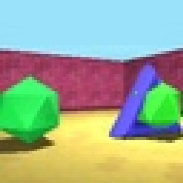
Published as a conference paper at ICLR 2020

In this work, we are interested in probabilistic generative models that can explain visual scenes
compositionally via several latent variables. This corresponds to fitting a probability distribution
pθ (x) with parameters
                  R     θ to the data. The compositional structure is captured by K latent variables
so that pθ (x) = pθ (x | z1:K )pθ (z1:K ) dz1:K . Models from this family can be optimised using
the variational auto-encoder (VAE) framework (Kingma & Welling, 2014; Rezende et al., 2014), by
maximising a variational lower bound on the model evidence (Jordan et al., 1999). Burgess et al.
(2019) and Greff et al. (2019) recently proposed two such models, MONet and IODINE, to decom-
pose visual scenes into meaningful objects. Both works leverage an analysis-by-synthesis approach
through the machinery of VAEs (Kingma & Welling, 2014; Rezende et al., 2014) to train these mod-
els without labelled supervision, e.g. in the form of ground truth segmentation masks. However, the
models have a factorised prior that treats scene components as independent. Thus, neither provides
an object-centric generation mechanism that accounts for relationships between constituent parts of
a scene, e.g. two physical objects cannot occupy the same location, prohibiting the component-wise
generation of novel scenes and restricting the utility of these approaches. Moreover, MONet embeds
a convolutional neural network (CNN) inside of an recurrent neural network (RNN) that is unrolled
for each scene component, which does not scale well to more complex scenes. Similarly, IODINE
utilises a CNN within an expensive, gradient-based iterative refinement mechanism.
Therefore, we introduce GENErative Scene Inference and Sampling (GENESIS) which is, to the best
of our knowledge, the first object-centric generative model of rendered 3D scenes capable of both de-
composing and generating scenes1 . Compared to previous work, this renders GENESIS significantly
more suitable for a wide range of applications in robotics and reinforcement learning. GENESIS
achieves this by modelling relationships between scene components with an expressive, autoregres-
sive prior that is learned alongside a sequential, amortised inference network. Importantly, sequen-
tial inference is performed in low-dimensional latent space, allowing all convolutional encoders and
decoders to be run in parallel to fully exploit modern graphics processing hardware.
We conduct experiments on three canonical and publicly available datasets: coloured Multi-dSprites
(Burgess et al., 2019), the GQN dataset (Eslami et al., 2018), and ShapeStacks (Groth et al., 2018).
The latter two are simulated 3D environments which serve as testing grounds for navigation and
object manipulation tasks, respectively. We show both qualitatively and quantitatively that in con-
trast to prior art, GENESIS is able to generate coherent scenes while also performing well on scene
decomposition. Furthermore, we use the scene annotations available for ShapeStacks to show the
benefit of utilising general purpose, object-centric latent representations from GENESIS for tasks
such as predicting whether a block tower is stable or not.
Code and models are available at https://github.com/applied-ai-lab/genesis.

2       R ELATED W ORK
Structured Models Several methods leverage structured latent variables to discover objects in im-
ages without direct supervision. CST- VAE (Huang & Murphy, 2015), AIR (Eslami et al., 2016),
SQAIR (Kosiorek et al., 2018), and SPAIR (Crawford & Pineau, 2019) use spatial attention to par-
tition scenes into objects. TAGGER (Greff et al., 2016), NEM (Greff et al., 2017), and R - NEM (van
Steenkiste et al., 2018a) perform unsupervised segmentation by modelling images as spatial mixture
models. SCAE (Kosiorek et al., 2019) discovers geometric relationships between objects and their
parts by using an affine-aware decoder. Yet, these approaches have not been shown to work on more
complex images, for example visual scenes with 3D spatial structure, occlusion, perspective distor-
tion, and multiple foreground and background components as considered in this work. Moreover,
none of them demonstrate the ability to generate novel scenes with relational structure.
While Xu et al. (2018) present an extension of Eslami et al. (2016) to generate images, their method
only works on binary images with a uniform black background and assumes that object bounding
boxes do not overlap. In contrast, we train GENESIS on rendered 3D scenes from Eslami et al. (2018)
and Groth et al. (2018) which feature complex backgrounds and considerable occlusion to perform
both decomposition and generation. Lastly, Xu et al. (2019) use ground truth pixel-wise flow fields
as a cue for segmenting objects or object parts. Similarly, GENESIS could be adapted to also leverage
temporal information which is a promising avenue for future research.

    1
        We use the terms “object” and “scene component” synonymously in this work.

                                                      2
Published as a conference paper at ICLR 2020

MON et & IODINE While this work is         most directly related to MONet (Burgess et al., 2019) and
IODINE (Greff et al., 2019), it sets itselfapart by introducing a generative model that captures rela-
tions between scene components with an autoregressive prior, enabling the unconditional generation
of coherent, novel scenes. Moreover, MONet relies on a deterministic attention mechanism rather
than utilising a proper probabilistic inference procedure. This implies that the training objective
is not a valid lower bound on the marginal likelihood and that the model cannot perform density
estimation without modification. Furthermore, this attention mechanism embeds a CNN in a RNN,
posing an issue in terms of scalability. These two considerations do not apply to IODINE, but IODINE
employs a gradient-based, iterative refinement mechanism which expensive both in terms of com-
putation and memory, limiting its practicality and utility. Architecturally, GENESIS is more similar
to MONet and does not require expensive iterative refinement as IODINE. Unlike MONet, though,
the convolutional encoders and decoders in GENESIS can be run in parallel, rendering the model
computationally more scalable to inputs with a larger number of scene components.
Adversarial Methods A few recent works have proposed to use an adversary for scene segmenta-
tion and generation. Chen et al. (2019) and Bielski & Favaro (2019) segment a single foreground
object per image and Arandjelović & Zisserman (2019) segment several synthetic objects superim-
posed on natural images. Azadi et al. (2019) combine two objects or an object and a background
scene in a sensible fashion and van Steenkiste et al. (2018b) can generate scenes with a potentially
arbitrary number of components. In comparison, GENESIS performs both inference and generation,
does not exhibit the instabilities of adversarial training, and offers a probabilistic formulation which
captures uncertainty, e.g. during scene decomposition. Furthermore, the complexity of GENESIS
increases with O(K), where K is the number of components, as opposed to the O(K 2 ) complexity
of the relational stage in van Steenkiste et al. (2018b).
Inverse Graphics A range of works formulate scene understanding as an inverse graphics problem.
These well-engineered methods, however, rely on scene annotations for training and lack probabilis-
tic formulations. For example, Wu et al. (2017b) leverage a graphics renderer to decode a structured
scene description which is inferred by a neural network. Romaszko et al. (2017) pursue a similar
approach but instead make use of a differentiable graphics render. Wu et al. (2017a) further employ
different physics engines to predict the movement of billiard balls and block towers.

3    G ENESIS : G ENERATIVE S CENE I NFERENCE AND S AMPLING
In this section, we first describe the generative model of GENESIS and a simplified variant called
GENESIS - S . This is followed by the associated inference procedures and two possible learning
objectives. GENESIS is illustrated in Figure 1 and Figure 2 shows the graphical model in comparison
to alternative methods. An illustration of GENESIS - S is included Appendix B.1, Figure 5.

Generative model Let x ∈ RH×W ×C be an image. We formulate the problem of image genera-
tion as a spatial Gaussian mixture model (GMM). That is, every Gaussian component k = 1, . . . , K
represents an image-sized scene component xk ∈ RH×W ×C . K ∈ N+ is the maximum number
of scene components. The corresponding mixing probabilities πk ∈ [0, 1]H×W indicate whether
the component is present at aPlocation in the image. The mixing probabilities are normalised across
scene components, i.e. ∀i,j k πi,j,k = 1, and can be regarded as spatial attention masks. Since
there are strong spatial dependencies between components, we formulate an autoregressive prior
distribution over mask variables zm
                                  k ∈R
                                         Dm
                                              which encode the mixing probabilities πk , as
                             K
                             Y                        K
                                                    Y
              pθ (zm
                   1:K ) =         pθ zm
                                       k | z m
                                             1:k−1  =   pθ (zm
                                                             k | uk )|uk =Rθ (zm
                                                                               k−1 ,uk−1 )
                                                                                           .        (1)
                             k=1                       k=1

The dependence on previous latents zm
                                    1:k−1 is implemented via an RNN Rθ with hidden state uk .

Next, we assume that the scene components xk are conditionally independent given their spatial allo-
cation in the scene. The corresponding conditional distribution over component variables zck ∈ RDc
which encode the scene components xk factorises as follows,
                                                           K
                                                           Y
                                    pθ (zc1:K | zm
                                                 1:K ) =         pθ (zck | zm
                                                                            k ).                    (2)
                                                           k=1

                                                      3
Published as a conference paper at ICLR 2020
Figure 1: GENESIS illustration. Given an image x, an encoder and an RNN compute the mask latents
zm
k . These are decoded to obtain the mixing probabilities πk . The image and individual masks are
concatenated to infer the component latents zck from which the scene components xk are decoded.
Now, the image likelihood is given by a mixture model,
K
X
p(x | zm c
1:K , z1:K ) = πk pθ (xk | zck ) , (3)
k=1
where the mixing probabilities πk = πθ (zm 1:k ) are created via a stick-breaking process ( SBP ) adapted
from Burgess et al. (2019) as follows, slightly overloading the π notation,
k−1
X K−1
X
π1 = πθ (zm 1 ), πk = 1 − πj πθ (zm
k ), πK = 1 − πj . (4)
j=1 j=1
Note that this step is not necessary for our model and instead one could use a softmax to normalise
masks as in Greff et al. (2019).
Finally, omitting subscripts, the full generative model can be written as
ZZ
pθ (x) = pθ (x | zc , zm )pθ (zc | zm )pθ (zm ) dzm dzc , (5)
where we assume that all conditional distributions are Gaussian. The Gaussian components of the
image likelihood have a fixed scalar standard deviation σx2 . We refer to this model as GENESIS. To
investigate whether separate latents for masks and component appearances are necessary for decom-
position, we consider a simplified model, GENESIS - S, with a single latent variable per component,
K
Y
pθ (z1:K ) = pθ (zk | z1:k−1 ). (6)
k=1
In this case, zk takes the role of zck in Equation (3) and of zm
k in Equation (4), while Equation (2) is
no longer necessary.
Approximate posterior We amortise inference by using an approximate posterior distribution
with parameters φ and a structure similar to the generative model. The full approximate posterior
reads as follows,
qφ (zc1:K , zm m c m
1:K | x) = qφ (z1:K | x) qφ (z1:K | x, z1:K ) , where
K K
Y Y (7)
qφ (zm qφ zm m
and qφ (zc1:K | x, zm qφ (zck | x, zm
1:K | x) = k | x, z1:k−1 , 1:K ) = 1:k ) ,
k=1 k=1
with the dependence on zm realised by an RNN Rφ . The RNN could, in principle, be shared with
1:k−1
the prior, but we have not investigated this option. All conditional distributions are Gaussian. For
QK
GENESIS - S , the approximate posterior takes the form qφ (z1:K | x) = k=1 qφ (zk | x, z1:k−1 ) .
4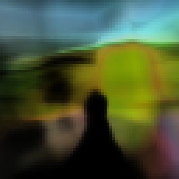
Published as a conference paper at ICLR 2020

        (a) VAE    (b) MONET       (c) IODINE            (d) GENESIS              (e) GENESIS-S

Figure 2: Graphical model of GENESIS compared to related methods. N denotes the number of
refinement iterations in IODINE. Unlike the other methods, both GENESIS variants explicitly model
dependencies between scene components.

Learning G ENESIS can be trained by maximising the evidence lower bound (ELBO) on the log-
marginal likelihood log pθ (x), given by
                                           pθ (x | zc , zm )pθ (zc | zm )pθ (zm )

        LELBO (x) = Eqφ (zc ,zm |x) log                                                                 (8)
                                               qφ (zc | zm , x)qφ (zm | x)
                  = Eqφ (zc ,zm |x) [log pθ (x | zc , zm )] − KL (qφ (zc , zm | x) || pθ (zc , zm )) .  (9)
However, this often leads to a strong emphasis on the likelihood term, while allowing the marginal
approximate posterior qφ (z) = Epdata (x) [qφ (z | x)] to drift away from the prior distribution, hence
increasing the KL-divergence. This also decreases the quality of samples drawn from the model.
To prevent this behaviour, we use the Generalised ELBO with Constrained Optimisation (GECO)
objective from Rezende & Viola (2018) instead, which changes the learning problem to minimising
the KL-divergence subject to a reconstruction constraint. Let C ∈ R be the minimum allowed
reconstruction log-likelihood, GECO then uses Lagrange multipliers to solve the following problem,
                      θ? , φ? = arg min KL (qφ (zc , zm | x) || pθ (zc , zm ))
                                       θ,φ
                                                                                                       (10)
                             such that Eqφ (zc ,zm |x) [log pθ (x | zc , zm )] ≥ C .

4     E XPERIMENTS
In this section, we present qualitative and quantitative results on coloured Multi-dSprites (Burgess
et al., 2019), the “rooms-ring-camera” dataset from GQN (Eslami et al., 2018) and the ShapeStacks
dataset (Groth et al., 2018). We use an image resolution of 64-by-64 for all experiments. The number
of components is set to K = 5, K = 7, and K = 9 for Multi-dSprites, GQN, and ShapeStacks,
respectively. More details about the datasets are provided in Appendix A. Implementation and
training details of all models are described in Appendix B.

4.1   C OMPONENT-W ISE S CENE G ENERATION

Unlike previous works, GENESIS has an autoregressive prior to capture intricate dependencies be-
tween scene components. Modelling these relationships is necessary to generate coherent scenes.
For example, different parts of the background need to fit together; we do not want to create com-
ponents such as the sky several times; and several physical objects cannot be in the same location.
GENESIS is able to generate novel scenes by sequentially sampling scene components from the prior
and conditioning each new component on those that have been generated during previous steps.
After training GENESIS and MONet on the GQN dataset, Figure 3 shows the component-by-
component generation process of novel scenes, corresponding to drawing samples from the respec-
tive prior distributions. More examples of generated scenes are shown in Figure 6, Appendix D.
With GENESIS, either an object in the foreground or a part of the background is generated at every
step and these components fit together to make up a semantically consistent scene that looks sim-
ilar to the training data. MONet, though, generates random artefacts at every step that do not form
a sensible scene. These results are striking but not surprising: MONet was not designed for scene
generation. The need for such a model is why we developed GENESIS.

                                                    5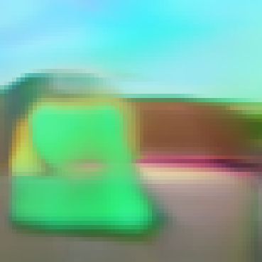
Published as a conference paper at ICLR 2020

                    Sample   = 1    = 2         = 3         = 4         = 5         = 6         = 7

Genesis: FID 80.5
MONet: FID 176.4

Figure 3: Component-by-component scene generation with GENESIS and MONet after training on the
GQN dataset. The first pane shows the final scene and the subsequent panes show the components
generated at each step. GENESIS first generates the sky and the floor, followed by individual objects,
and finally distinct parts of the wall in the background to compose a coherent scene. MONet, in
contrast, only generates incomplete components that do not fit together.

Notably, GENESIS pursues a consistent strategy for scene generation: Step one generates the floor
and the sky, defining the layout of the scene. Steps two to four generate individual foreground
objects. Some of these slots remain empty if less than three objects are present in the scene. The
final three steps generate the walls in the background. We conjecture that this strategy evolves during
training as the floor and sky constitute large and easy to model surfaces that have a strong impact
on the reconstruction loss. Finally, we observe that some slots contain artefacts of the sky at the top
of the wall boundaries. We conjecture this is due to the fact that the mask decoder does not have
skip connections as typically used in segmentation networks, making it difficult for the model to
predict sharp segmentation boundaries. Scenes generated by GENESIS - S are shown in Figure 8 and
Figure 9, Appendix D. While GENESIS - S does separate the foreground objects from the background,
it generates them in one step and the individual background components are not very interpretable.

                                                  6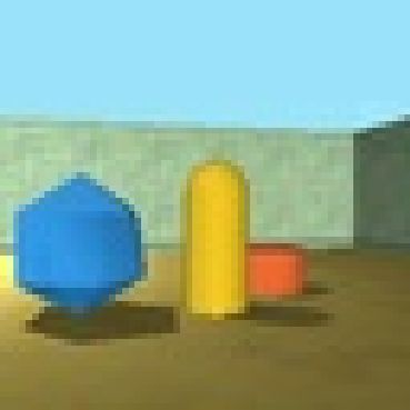
Published as a conference paper at ICLR 2020

4.2       I NFERENCE OF S CENE C OMPONENTS

Like MONet and IODINE, which were designed for unsupervised scene decomposition, GENESIS is
also able to segment scenes into meaningful components. Figure 4 compares the decomposition
of two images from the GQN dataset with GENESIS and MONet. Both models follow a similar
decomposition strategy, but MONet fails to disambiguate one foreground object in the first example
and does not reconstruct the background in as much detail in the second example. In Appendix E,
Figure 10 illustrates the ability of both methods to disambiguate objects of the same colour and
Figure 11 shows scene decomposition with GENESIS - S.
Following Greff et al. (2019), we quantify segmentation performance with the Adjusted Rand Index
(ARI) of pixels overlapping with ground truth foreground objects. We computed the ARI on 300
random images from the ShapeStacks test set for five models trained with different random seeds.
GENESIS achieves an ARI of 0.73 ± 0.03 which is better than 0.63 ± 0.07 for MON et. This metric,
however, does not penalise objects being over-segmented, which can give a misleading impression
with regards to segmentation quality. This is illustrated in Figure 13, Appendix E.
Inspired by Arbelaez et al. (2010), we thus propose to use the segmentation covering (SC) of the
ground truth foreground objects by the predicted masks. This involves taking a weighted mean over
mask pairs, putting a potentially undesirable emphasis on larger objects. We therefore also consider
taking an unweighted mean (mSC). For the same 300 images from the ShapeStacks test set and five
different random seeds, GENESIS (SC: 0.64 ± 0.08, mSC: 0.60 ± 0.09) again outperforms MONet
(SC: 0.52 ± 0.09, mSC: 0.49 ± 0.09). More details are provided in Appendix C.

          Input   Reconstruction   = 1    = 2         = 3      = 4        = 5        = 6        = 7
Genesis
MONet
Genesis
MONet

Figure 4: Step-by-step decomposition of the same scene from GQN with GENESIS and MONet.
Unlike MONet, GENESIS clearly differentiates individual objects in the first example. In the second
example, GENESIS captures the fine-grained pattern of the wall in the background better than MONet.

4.3       E VALUATION OF U NSUPERVISED R EPRESENTATION U TILITY

Using a subset of the available labelled training images from ShapeStacks, we train a set of clas-
sifiers on the representations learned by GENESIS and several baselines to evaluate how well these
representations capture the ground truth scene state. In particular, we consider three tasks: (1) Is
a tower stable or not? (2) What is the tower’s height in terms of the number of blocks? (3) What
is the camera viewpoint (out of 16 possibilities)? Tower stability is a particularly interesting prop-
erty as it depends on in fine-grained object information and the relative positioning of objects. We
selected the third task as learning scene representations from different views has previously been
prominently explored in Eslami et al. (2018). We compare GENESIS and GENESIS - S against three
baselines: MONet, a VAE with a spatial broadcast decoder (BD - VAE) and a VAE with a deconvo-
lutional decoder (DC - VAE). The results are summarised in Table 1. The architectural details of
the baselines are described in Appendix B.2 and Appendix B.3. The implementation details of the
classifiers are provided in Appendix B.5.

                                                  7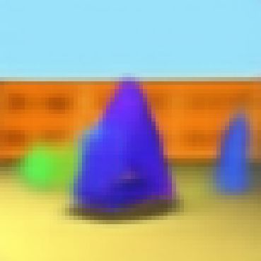
Published as a conference paper at ICLR 2020

Both GENESIS and GENESIS - S perform better than than the baselines at predicting tower stability
and their accuracies on predicting the height of the towers is only outperformed by MONet. We
conjecture that MONet benefits here by its deterministic segmentation network. Overall, this cor-
roborates the intuition that object-centric representations are indeed beneficial for these tasks which
focus on the foreground objects. We observe that the BD - VAE does better than the DC - VAE on all
three tasks, reflecting the motivation behind its design which is aimed at better disentangling the un-
derlying factors of variation in the data (Watters et al., 2019b). All models achieve a high accuracy at
predicting the camera view. Finally, we note that none of models reach the stability prediction accu-
racies reported in Groth et al. (2018) which were obtained with an Inception-v4 classifier (Szegedy
et al., 2017). This is not surprising considering that only a subset the training images is used for
training the classifiers without data augmentation and at a reduced resolution.

          Table 1: Classification accuracy in % on the test sets of the ShapeStacks tasks.

         Task        GENESIS      GENESIS - S   MON et      BD - VAE     DC - VAE     Random
         Stability     64.0         63.2         59.6         60.1         59.0         50.0
         Height        80.3         80.8         88.4         78.6         67.5         22.8
         View          99.3         99.7         99.5         99.7         99.1         6.25

4.4   Q UANTIFYING S AMPLE Q UALITY

In order to quantify the quality of generated scenes, Table 2 summarises the Fréchet Inception Dis-
tances (FIDs) (Heusel et al., 2017) between 10,000 images generated by GENESIS as well several
baselines and 10,000 images from the Multi-dSprites and the GQN test sets, respectively. The two
GENESIS variants achieve the best FID on both datasets. While GENESIS - S performs better than
GENESIS on GQN, Figure 8 and Figure 9 in Appendix D show that individual scene components
are less interpretable and that intricate background patterns are generated at the expense of sensible
foreground objects. It is not surprising that the FIDs for MONet are relatively large given that it
was not designed for generating scenes. Interestingly, the DC - VAE achieves a smaller FID on GQN
than the BD - VAE. This is surprising given that the BD - VAE representations are more useful for the
ShapeStacks classification tasks. Given that the GQN dataset and ShapeStacks are somewhat simi-
lar in structure and appearance, this indicates that while FID correlates with perceptual similarity, it
does not necessarily correlate with the general utility of the learned representations for downstream
tasks. We include scenes sampled from the BD - VAE and the DC - VAE in Figure 7, Appendix D, where
we observe that the DC - VAE models the background fairly well while foreground objects are blurry.

             Table 2: Fréchet Inception Distances for GENESIS and baselines on GQN.

           Dataset            GENESIS      GENESIS - S   MON et        BD - VAE     DC - VAE
           Multi-dSprites       24.9         28.2          92.7          89.8        100.5
           GQN                  80.5         70.2         176.4         145.5         82.5

5     C ONCLUSIONS
In this work, we propose a novel object-centric latent variable model of scenes called GENESIS. We
show that GENESIS is, to the best of our knowledge, the first unsupervised model to both decompose
rendered 3D scenes into semantically meaningful constituent parts, while at the same time being able
to generate coherent scenes in a component-wise fashion. This is achieved by capturing relationships
between scene components with an autoregressive prior that is learned alongside a computationally
efficient sequential inference network, setting GENESIS apart from prior art. Regarding future work,
an interesting challenge is to scale GENESIS to more complex datasets and to employ the model
in robotics or reinforcement learning applications. To this end, it will be necessary to improve
reconstruction and sample quality, reduce computational cost, and to scale the model to higher
resolution images. Another potentially promising research direction is to adapt the formulation to
only model parts of the scene that are relevant for a certain task.

                                                    8
Published as a conference paper at ICLR 2020

ACKNOWLEDGMENTS
This research was supported by an EPSRC Programme Grant (EP/M019918/1), an EPSRC DTA
studentship, and a Google studentship. The authors would like to acknowledge the use of the
University of Oxford Advanced Research Computing (ARC) facility in carrying out this work,
http://dx.doi.org/10.5281/zenodo.22558, and the use of Hartree Centre resources.
The authors would like to thank Yizhe Wu for his help with re-implementing MONet, Oliver Groth
for his support with the GQN and ShapeStacks datasets, and Rob Weston for proof reading the paper.

R EFERENCES
Relja Arandjelović and Andrew Zisserman. Object Discovery with a Copy-Pasting GAN. arXiv
  preprint arXiv:1905.11369, 2019.
Pablo Arbelaez, Michael Maire, Charless Fowlkes, and Jitendra Malik. Contour Detection and Hier-
  archical Image Segmentation. IEEE Transactions on Pattern Analysis and Machine Intelligence,
  2010.
Samaneh Azadi, Deepak Pathak, Sayna Ebrahimi, and Trevor Darrell. Compositional GAN: Learn-
  ing Image-Conditional Binary Composition. arXiv preprint arXiv:1807.07560, 2019.
Rianne van den Berg, Leonard Hasenclever, Jakub M Tomczak, and Max Welling. Sylvester Nor-
  malizing Flows for Variational Inference. Conference on Uncertainty in Artificial Intelligence,
  2018.
Adam Bielski and Paolo Favaro. Emergence of Object Segmentation in Perturbed Generative Mod-
  els. arXiv preprint arXiv:1905.12663, 2019.
Andrew Brock, Jeff Donahue, and Karen Simonyan. Large Scale GAN Training for High Fidelity
  Natural Image Synthesis. arXiv preprint arXiv:1809.11096, 2018.
Christopher P Burgess, Loic Matthey, Nicholas Watters, Rishabh Kabra, Irina Higgins, Matt
  Botvinick, and Alexander Lerchner. MONet: Unsupervised Scene Decomposition and Repre-
  sentation. arXiv preprint arXiv:1901.11390, 2019.
Mickaël Chen, Thierry Artières, and Ludovic Denoyer. Unsupervised Object Segmentation by Re-
 drawing. arXiv preprint arXiv:1905.13539, 2019.
Djork-Arné Clevert, Thomas Unterthiner, and Sepp Hochreiter. Fast and Accurate Deep Network
  Learning by Exponential Linear Units (ELUs). International Conference on Learning Represen-
  tations, 2016.
Pierre Comon. Independent Component Analysis. In J-L.Lacoume (ed.), Higher-Order Statistics,
  pp. 29–38. Elsevier, 1992.
Eric Crawford and Joelle Pineau. Spatially Invariant Unsupervised Object Detection with Convolu-
  tional Neural Networks. AAAI Conference on Artificial Intelligence, 2019.
Yann N Dauphin, Angela Fan, Michael Auli, and David Grangier. Language Modeling with Gated
  Convolutional Networks. International Conference on Machine Learning, 2017.
SM Ali Eslami, Nicolas Heess, Theophane Weber, Yuval Tassa, David Szepesvari, Geoffrey E Hin-
 ton, et al. Attend, Infer, Repeat: Fast Scene Understanding with Generative Models. Neural
 Information Processing Systems, 2016.
SM Ali Eslami, Danilo Jimenez Rezende, Frederic Besse, Fabio Viola, Ari S Morcos, Marta Gar-
 nelo, Avraham Ruderman, Andrei A Rusu, Ivo Danihelka, Karol Gregor, et al. Neural Scene
 Representation and Rendering. Science, 2018.
Karl Friston. A Theory of Cortical Responses. Philosophical Transactions of the Royal Society B:
  Biological Sciences, 360(1456):815–836, 2005.
Xavier Glorot, Antoine Bordes, and Yoshua Bengio. Deep Sparse Rectifier Neural Networks. Inter-
  national Conference on Artificial Intelligence and Statistics, 2011.

                                                9
Published as a conference paper at ICLR 2020

Klaus Greff, Antti Rasmus, Mathias Berglund, Tele Hao, Harri Valpola, and Jürgen Schmidhuber.
  Tagger: Deep Unsupervised Perceptual Grouping. Neural Information Processing Systems, 2016.

Klaus Greff, Sjoerd van Steenkiste, and Jürgen Schmidhuber. Neural Expectation Maximization.
  Neural Information Processing Systems, 2017.

Klaus Greff, Raphaël Lopez Kaufmann, Rishab Kabra, Nick Watters, Chris Burgess, Daniel Zo-
  ran, Loic Matthey, Matthew Botvinick, and Alexander Lerchner. Multi-Object Representation
  Learning with Iterative Variational Inference. International Conference on Machine Learning,
  2019.

Karol Gregor, Danilo Jimenez Rezende, Frederic Besse, Yan Wu, Hamza Merzic, and Aaron van den
  Oord. Shaping Belief States with Generative Environment Models for RL. arXiv preprint
  arXiv:1906.09237, 2019.

Kalanit Grill-Spector and Rafael Malach. The Human Visual Cortex. Annual Review of Neuro-
  science, 27(1):649–677, 2004.

Oliver Groth, Fabian B Fuchs, Ingmar Posner, and Andrea Vedaldi. ShapeStacks: Learning Vision-
  Based Physical Intuition for Generalised Object Stacking. European Conference on Computer
  Vision, 2018.

David Ha and Jürgen Schmidhuber. World Models. Neural Information Processing Systems, 2018.

Martin Heusel, Hubert Ramsauer, Thomas Unterthiner, Bernhard Nessler, and Sepp Hochreiter.
 GANs Trained by a Two Time-Scale Update Rule Converge to a Local Nash Equilibrium. Neural
 Information Processing Systems, 2017.

Sepp Hochreiter and Jürgen Schmidhuber. Long Short-Term Memory. Neural Computation, 1997.

Jonathan Huang and Kevin Murphy. Efficient Inference in Occlusion-Aware Generative models of
  Images. arXiv preprint arXiv:1511.06362, 2015.

D. H. Hubel and T. N. Wiesel. Receptive Fields and Functional Architecture of Monkey Striate
  Cortex. The Journal of Physiology, 195(1):215–243, 1968.

Sergey Ioffe and Christian Szegedy. Batch Normalization: Accelerating Deep Network Training by
  Reducing Internal Covariate Shift. International Conference on Machine Learning, 2015.

Michael I Jordan, Zoubin Ghahramani, Tommi S Jaakkola, and Lawrence K Saul. An Introduction
 to Variational Methods for Graphical Models. Machine Learning, 37(2):183–233, 1999.

Diederik P Kingma and Jimmy Ba. Adam: A Method for Stochastic Optimization. International
  Conference on Learning Representations, 2015.

Diederik P Kingma and Max Welling. Auto-Encoding Variational Bayes. International Conference
  on Learning Representations, 2014.

Adam Kosiorek, Hyunjik Kim, Yee Whye Teh, and Ingmar Posner. Sequential Attend, Infer, Repeat:
  Generative Modelling of Moving Objects. Neural Information Processing Systems, 2018.

Adam R Kosiorek, Sara Sabour, Yee Whye Teh, and Geoffrey E Hinton. Stacked Capsule Autoen-
  coders. arXiv preprint arXiv:1906.06818, 2019.

Loic Matthey, Irina Higgins, Demis Hassabis, and Alexander Lerchner. dSprites: Disentanglement
  Testing Sprites Dataset. https://github.com/deepmind/dsprites-dataset/, 2017.

Bruno A. Olshausen and David J. Field. Emergence of Simple-Cell Receptive Field Properties by
  Learning a Sparse Code for Natural Images. Nature, 381:607–609, 1996.

Niki Parmar, Ashish Vaswani, Jakob Uszkoreit, Łukasz Kaiser, Noam Shazeer, Alexander Ku, and
  Dustin Tran. Image Transformer. International Conference on Machine Learning, 2018.

                                               10
Published as a conference paper at ICLR 2020
Rajesh P. N. Rao and Dana H. Ballard. Predictive Coding in the Visual Cortex: A Functional
Interpretation of Some Extra-Classical Receptive-Field Effects. Nature Neuroscience, 2(1):79–
87, 1999.
Danilo Jimenez Rezende and Fabio Viola. Taming VAEs. arXiv preprint arXiv:1810.00597, 2018.
Danilo Jimenez Rezende, Shakir Mohamed, and Daan Wierstra. Stochastic Backpropagation and
Approximate Inference in Deep Generative Models. International Conference on Machine Learn-
ing, 2014.
Lukasz Romaszko, Christopher KI Williams, Pol Moreno, and Pushmeet Kohli. Vision-as-Inverse-
Graphics: Obtaining a Rich 3D Explanation of a Scene from a Single Image. In IEEE Interna-
tional Conference on Computer Vision, 2017.
Adam Santoro, David Raposo, David G. T. Barrett, Mateusz Malinowski, Razvan Pascanu, Peter W.
Battaglia, and Timothy P. Lillicrap. A Simple Neural Network Module for Relational Reasoning.
Neural Information Processing Systems, 2017.
Christian Szegedy, Sergey Ioffe, Vincent Vanhoucke, and Alexander A Alemi. Inception-V4,
Inception-Resnet and the Impact of Residual Connections on Learning. AAAI Conference on
Artificial Intelligence, 2017.
Naftali Tishby, Fernando C Pereira, and William Bialek. The Information Bottleneck Method. arXiv
preprint arXiv:physics/0004057, 2000.
Sjoerd van Steenkiste, Michael Chang, Klaus Greff, and Jürgen Schmidhuber. Relational Neural
Expectation Maximization: Unsupervised Discovery of Objects and their Interactions. arXiv
preprint arXiv:1802.10353, 2018a.
Sjoerd van Steenkiste, Karol Kurach, and Sylvain Gelly. A Case for Object Compositionality in
Deep Generative Models of Images. NeurIPS Workshop on Modeling the Physical World: Learn-
ing, Perception, and Control, 2018b.
Sjoerd van Steenkiste, Francesco Locatello, Jurgen Schmidhuber, and Olivier Bachem. Are
Disentangled Representations Helpful for Abstract Visual Reasoning? arXiv preprint
arXiv:1905.12506, 2019.
Brian A. Wandell. Foundations of Vision. Sinauer Associates, 1995.
Nicholas Watters, Loic Matthey, Matko Bosnjak, Christopher P Burgess, and Alexander Lerchner.
COBRA: Data-Efficient Model-Based RL through Unsupervised Object Discovery and Curiosity-
Driven Exploration. arXiv preprint arXiv:1905.09275, 2019a.
Nicholas Watters, Loic Matthey, Christopher P Burgess, and Alexander Lerchner. Spatial Broadcast
Decoder: A Simple Architecture for Learning Disentangled Representations in VAEs. arXiv
preprint arXiv:1901.07017, 2019b.
Jiajun Wu, Erika Lu, Pushmeet Kohli, Bill Freeman, and Josh Tenenbaum. Learning to See Physics
via Visual De-Animation. Neural Information Processing Systems, 2017a.
Jiajun Wu, Joshua B Tenenbaum, and Pushmeet Kohli. Neural Scene De-rendering. IEEE Confer-
ence on Computer Vision and Pattern Recognition, pp. 699–707, 2017b.
Kun Xu, Chongxuan Li, Jun Zhu, and Bo Zhang. Multi-Objects Generation with Amortized Struc-
tural Regularization. Neural Information Processing Systems, 2018.
Zhenjia Xu, Zhijian Liu, Chen Sun, Kevin Murphy, William T Freeman, Joshua B Tenenbaum,
and Jiajun Wu. Unsupervised Discovery of Parts, Structure, and Dynamics. arXiv preprint
arXiv:1903.05136, 2019.
11Published as a conference paper at ICLR 2020
A DATASETS
Multi-dSprites (Burgess et al., 2019) Images contain between one and four randomly se-
lected “sprites” from Matthey et al. (2017), available at https://github.com/deepmind/
dsprites-dataset. For each object and the background, we randomly select one of five dif-
ferent, equally spread values for each of the three colour channels and generate 70,000 images. We
set aside 10,000 for validation and testing each. The script for generating this data will be released
with the rest of our code.
GQN (Eslami et al., 2018) The “rooms-ring-camera” dataset includes simulated 3D scenes of a
square room with different floor and wall textures, containing one to three objects of various shapes
and sizes. It can be downloaded from https://github.com/deepmind/gqn-datasets.
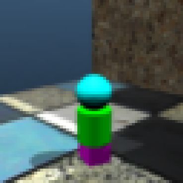
ShapeStacks (Groth et al., 2018) Images show simulated block towers of different heights (two to
six blocks). Individual blocks can have different shapes, sizes, and colours. Scenes have annotations
for: stability of the tower (binary), number of blocks (two to six), properties of individual blocks,
locations in the tower of centre-of-mass violations and planar surface violations, wall and floor
textures (five each), light presets (five), and camera view points (sixteen). More details about the
dataset and download links can be found at https://shapestacks.robots.ox.ac.uk/.
B I MPLEMENTATION D ETAILS
B.1 G ENESIS A RCHITECTURE
We use the architecture from Berg et al. (2018) to encode and decode zm k with the only modification
of applying batch normalisation (Ioffe & Szegedy, 2015) before the GLU non-linearities (Dauphin
et al., 2017). The convolutional layers in the encoder and decoder have five layers with size-5
kernels, strides of [1, 2, 1, 2, 1], and filter sizes of [32, 32, 64, 64, 64] and [64, 32, 32, 32, 32],
respectively. Fully-connected layers are used at the lowest resolution.
The encoded image is passed to a long short-term memory (LSTM) cell (Hochreiter & Schmidhuber,
1997) followed by a linear layer to compute the mask latents zm k of size 64. The LSTM state size
is twice the latent size. Importantly, unlike the analogous counterpart in MONet, the decoding of
zm m m
k is performed in parallel. The autoregressive prior pθ zk | z1:k−1 is implemented as an LSTM
with 256 units. The conditional distribution pθ (zck | zm
k ) is parameterised by a multilayer perceptron
(MLP) with two hidden layers, 256 units per layer, and ELUs (Clevert et al., 2016). We use the same
component VAE featuring a spatial broadcast decoder as MONet to encode and decode zkc , but we
replace RELUs (Glorot et al., 2011) with ELUs.
For GENESIS - S, as illustrated in Figure 5, the encoder of zk is the same as for zm k above and the
decoder from Berg et al. (2018) is again used to compute the mixing probabilities. However, GEN -
ESIS - S also has a second decoder with spatial broadcasting to obtain the scene components xk from
zk . We found the use of two different decoders to be important for GENESIS - S in order for the model
to decompose the input.
Figure 5: GENESIS-S overview. Given an image x, an encoder and an RNN compute latent variables
zk . These are decoded to directly obtain the mixing probabilities πk and the scene components xk .
12Published as a conference paper at ICLR 2020
B.2 MON ET BASELINES
We followed the provided architectural details described in Burgess et al. (2019). Regarding un-
specified details, we employ an attention network with [32, 32, 64, 64, 64] filters in the encoder and
the reverse in the decoder. Furthermore, we normalise the mask prior with a softmax function to
compute the KL-divergence between mask posterior and prior distributions.
B.3 VAE BASELINES
Both the BD - VAE and the DC - VAE have a latent dimensionality of 64 and the same encoder as in
Berg et al. (2018). The DC - VAE also uses the decoder from Berg et al. (2018). The BD - VAE has the
same spatial broadcast decoder with ELUs as GENESIS, but with twice the number of filters to enable
a better comparison.
B.4 O PTIMISATION
The scalar standard deviation of the Gaussian image likelihood components is set to σx = 0.7. We
use GECO (Rezende & Viola, 2018) to balance the reconstruction and KL divergence terms in the
loss function. The goal for the reconstruction error is set to 0.5655, multiplied by the image dimen-
sions and number of colour channels. We deliberately choose a comparatively weak reconstruction
constraint for the GECO objective to emphasise KL minimisation and sample quality. For the remain-
ining GECO hyperparameters, the default value of α = 0.99 is used and the step size for updating β
is set to 10−5 . We increase the step size to 10−4 when the reconstruction constraint is satisfied to
accelerate optimisation as β tended to undershoot at the beginning of training.
All models are trained for 5 ∗ 105 iterations with a batch size of 32 using the ADAM optimiser
(Kingma & Ba, 2015) and a learning rate of 10−4 . With these settings, training GENESIS takes
about two days on a single GPU. However, we expect performance to improve with further training.
This particularly extends to training GENESIS on ShapeStacks where 5 ∗ 105 training iterations are
not enough to achieve good sample quality.
B.5 S HAPE S TACKS C LASSIFIERS
Multilayer perceptrons (MLPs) with one hidden layer, 512 units, and ELU activations are used for
classification. The classifiers are trained for 100 epochs on 50,000 labelled examples with a batch
size of 128 using a cross-entropy loss, the ADAM optimiser, and a learning rate of 10−4 . As inputs
to the classifiers, we concatenate zm c
k and zk for GENESIS , zk for GENESIS - S , and the component
VAE latents for the two MON et variants.
C S EGMENTATION C OVERING
Following Arbelaez et al. (2010), the segmentation covering (SC) is based on the intersection over
union (IOU) between pairs of segmentation masks from two sets S and S 0 . In this work, we consider
S to be the segmentation masks of the ground truth foreground objects and S 0 to be the predicted
segmentation masks. The covering of S by S 0 is defined as:
1 X
C(S 0 → S) = P |R| max 0
IOU (R, R ), (11)
R∈S |R| R∈S
R0 ∈S 0
where |R| denotes the number of pixels belonging to mask R. Note that this formulation is slightly
more general than the one in Arbelaez et al. (2010) which assumes that masks in S are non-
overlapping and cover the entire image. The above takes a weighted mean over IOU values, pro-
portional to the number of pixels of the masks being covered. To give equal importance to masks of
different sizes, we also consider taking an unweighted mean (mSC):
1 X
Cm (S 0 → S) = max IOU(R, R0 ), (12)
|S| R0 ∈S 0
R∈S
where |S| denotes the number of non-empty masks in S. Importantly and unlike the ARI, both
segmentation covering variations penalise the over-segmentation of ground truth objects as this de-
creases the IOU for a pair of masks. This is illustrated in Figure 13, Appendix E.
13Published as a conference paper at ICLR 2020
D C OMPONENT-W ISE S CENE G ENERATION - GQN
Genesis: FID 80.5
MONet: FID 176.4
Figure 6: Randomly selected scenes generated by GENESIS and MONet after training on the GQN
dataset. Images sampled from GENESIS contain clearly distinguishable foreground objects and back-
grounds. Samples from MONet, however, are mostly incoherent.
BD-VAE: FID 145.5
DC-VAE: FID 82.5
Figure 7: Randomly selected scenes generated by the BD-VAE and the DC-VAE after training on
the GQN dataset; shown for comparison. The DC-VAE generates decent scene backgrounds but
foreground objects are blurry.
14Published as a conference paper at ICLR 2020
Sample = 1 = 2 = 3 = 4 = 5 = 6 = 7
Genesis-S: FID 70.2
Figure 8: Component-by-component scene generation with GENESIS - S after training on the GQN
dataset. While GENESIS - S nominally achieves the best FID in Table 2, this appears to be due to
the generation of high fidelity background patterns rather than appropriate foreground objects. Fur-
thermore, unlike the components generated by GENESIS at every step in Figure 3, the components
generated by GENESIS - S are not very interpretable.
Genesis-S: FID 70.2
Figure 9: Randomly selected scenes generated by GENESIS - S after training on the GQN dataset.
15Published as a conference paper at ICLR 2020
E I NFERENCE OF S CENE C OMPONENTS
Input Reconstruction = 1 = 2 = 3 = 4 = 5 = 6 = 7
Genesis
MONet
Figure 10: Step-by-step decomposition of a scene from GQN with GENESIS and MONet. Two objects
with the same shape and colour are successfully identified by both models. While colour and texture
are useful cues for decomposition, this example shows that both models perform something more
useful than merely identifying regions of similar colour.
Input Reconstruction = 1 = 2 = 3 = 4 = 5 = 6 = 7
Genesis-S
Figure 11: Step-by-step decomposition of the same scenes as in Figure 4 and Figure 10 with
GENESIS - S . While the foreground objects are distinguished from the background, they are explained
together in the first step. Subsequent steps reconstruct the background in a haphazard fashion.
16Published as a conference paper at ICLR 2020
= 1 = 2 = 3 = 4 = 5 = 6
Genesis
Input Reconstruction
= 7 = 8 = 9
= 1 = 2 = 3 = 4 = 5 = 6
MONet
Input Reconstruction
= 7 = 8 = 9
Figure 12: A ShapeStacks tower is decomposed by GENESIS and MONet. Compared to the GQN
dataset, both methods struggle to segment the foreground objects properly. GENESIS captures the
purple shape and parts of the background wall in step k = 4. MONet explains the green shape,
the cyan shape, and parts of floor in step k = 9. This is reflected in the foreground ARI and
segmentation covering for GENESIS (ARI: 0.82, SC: 0.68, mSC: 0.58) and MONet (ARI: 0.39, SC:
0.26, mSC: 0.35); the latter being lower as the green and cyan shapes are not separated.
= 1 = 2 = 3 = 4 = 5 = 6
Genesis
Input Reconstruction
= 7 = 8 = 9
= 1 = 2 = 3 = 4 = 5 = 6
MONet
Input Reconstruction
= 7 = 8 = 9
Figure 13: In this example, GENESIS (ARI: 0.83, SC: 0.83, mSC: 0.83) segments the four foreground
objects properly. MONet (ARI: 0.89, SC: 0.47, mSC: 0.50), however, merges foreground objects and
background again in steps k = 2 and k = 9. Despite the inferior decomposition, the ARI for MONet
is higher than for GENESIS. This is possible as the ARI does not penalise the over-segmentation of
the foreground objects, highlighting its limitations for evaluating unsupervised instance segmenta-
tion. The segmentation covering, however, reflects the quality of the segmentatioin masks properly.
17You can also read