GeoNet: Deep Geodesic Networks for Point Cloud Analysis
←
→
Page content transcription
If your browser does not render page correctly, please read the page content below
GeoNet: Deep Geodesic Networks for Point Cloud Analysis

                                             Tong He1 , Haibin Huang2 , Li Yi3 , Yuqian Zhou4 , Chihao Wu2 , Jue Wang2 , Stefano Soatto1
                                                                 1
                                                                   UCLA 2 Megvii (Face++) 3 Stanford 4 UIUC

                                                                 Abstract
arXiv:1901.00680v1 [cs.CV] 3 Jan 2019

                                            Surface-based geodesic topology provides strong cues
                                        for object semantic analysis and geometric modeling. How-
                                        ever, such connectivity information is lost in point clouds.
                                        Thus we introduce GeoNet, the first deep learning archi-
                                        tecture trained to model the intrinsic structure of surfaces
                                        represented as point clouds. To demonstrate the applica-
                                        bility of learned geodesic-aware representations, we pro-
                                        pose fusion schemes which use GeoNet in conjunction with
                                        other baseline or backbone networks, such as PU-Net and
                                                                                                              Figure 1. Our method takes a point cloud as input, and outputs rep-
                                        PointNet++, for down-stream point cloud analysis. Our
                                                                                                              resentations used for multiple tasks including upsampling, normal
                                        method improves the state-of-the-art on multiple represen-            estimation, mesh reconstruction, and shape classification.
                                        tative tasks that can benefit from understandings of the un-
                                        derlying surface topology, including point upsampling, nor-
                                        mal estimation, mesh reconstruction and non-rigid shape               lying surface topology as well as object geometry, and pro-
                                        classification.                                                       pose methods that leverage the learned topological features
                                                                                                              for geodesic-aware point cloud analysis. The representa-
                                        1. Introduction                                                       tion should capture various topological patterns of a point
                                                                                                              cloud and the method of leveraging these geodesic features
                                        Determining neighborhood relationship among points in a               should not alter the data stream, so our representation can
                                        point cloud, known as topology estimation, is an important            be learned jointly and used in conjunction with the state-of-
                                        problem since it indicates the underlying point cloud struc-          the-art baseline or backbone models (e.g. PU-Net, Point-
                                        ture, which could further reveal the point cloud semantics            Net++ [37, 27, 28]) that feed the raw data through, with no
                                        and functionality. Consider the red inset in Fig. 1: the two          information loss to further stages of processing.
                                        clusters of points, though seemingly disconnected, should                For the first goal, we propose a geodesic neighborhood
                                        indeed be connected to form a chair leg, which supports the           estimation network (GeoNet) to learn deep geodesic repre-
                                        whole chair. On the other hand, the points on opposite sides          sentations using the ground truth geodesic distance as su-
                                        of a chair seat, though spatially very close to each other,           pervision signals. As illustrated in Fig. 2, GeoNet consists
                                        should not be connected to avoid confusing the sittable up-           of two modules: an autoencoder that extracts a feature vec-
                                        per surface with the unsittable lower side. Determining such          tor for each point and a geodesic matching (GM) layer that
                                        topology appears to be a very low-level endeavor but in real-         acts as a learned kernel function for estimating geodesic
                                        ity it requires global, high-level knowledge, making it a very        neighborhoods using the latent features. Due to the super-
                                        challenging task. Still, from the red inset in Fig. 1, we could       vised geodesic training process, intermediates features of
                                        draw the conclusion that the two stumps are connected only            the GM layer contain rich information of the point cloud
                                        after we learn statistical regularities from a large number           topology and intrinsic surface attributes. We note that the
                                        of point clouds and observe many objects of this type with            representation, while trained on geodesic distances, does
                                        connected elongated vertical elements extending from the              not by construction produce geodesics (e.g. symmetry, tri-
                                        body to the ground. This motivates us to adopt a learning             angle inequality, etc.). The goal of the representation is to
                                        approach to capture the topological structure within point            inform subsequent stages of processing of the global geom-
                                        clouds.                                                               etry and topology, and is not to conduct metric computa-
                                            Our primary goals in this paper are to develop represen-          tions directly.
                                        tations of point cloud data that are informed by the under-              For the second task, as shown in Fig. 3, we propose

                                                                                                          1
geodesic fusion schemes to integrate GeoNet into the state-      have much lower time complexity than the surface travers-
of-the-art network architectures designed for different tasks.   ing methods. For a 20000-vertex mesh, computing its all-
Specifically, we present PU-Net fusion (PUF) for point           pair geodesic distances can take several days using [35]
cloud upsampling, and PointNet++ fusion (POF) for normal         while [19] only uses about 1 minute on CPU. When a mesh
estimation, mesh reconstruction as well as non-rigid shape       is dense, the edge-constrained shortest path methods gen-
classification. Through experiments, we demonstrate that         erate low-error geodesic estimates. Thus in our work, we
the learned geodesic representations from GeoNet are bene-       apply [19] to compute the ground truth geodesic distance.
ficial for both geometric and semantic point cloud analyses.         Point upsampling. Previous methods can be summa-
    In summary, in this paper we propose an approach for         rized into two categories. i) Optimization based meth-
learning deep geodesic-aware representations from point          ods [1, 23, 18], championed by [1], which interpolates a
clouds and leverage the results for various point set anal-      dense point set from vertices of a Voronoi diagram in the
yses. Our contributions are:                                     local tangent space. Then [23] proposes a locally opti-
                                                                 mal projection (LOP) operator for point cloud resampling
  • We present, to the best of our knowledge, the first deep     and mesh reconstruction leveraging an L1 median. For im-
    learning method, GeoNet, that ingests point clouds and       proving robustness to point cloud density variations, [18]
    learns representations which are informed by the in-         presents a weighted LOP. These methods all make strong
    trinsic structure of the underlying point set surfaces.      assumptions, such as surface smoothness, and are not data-
                                                                 driven, and therefore have limited applications in practice.
  • To demonstrate the applicability of learned geodesic         ii) Deep learning based methods. To apply the (graph) con-
    representations, we develop network fusion architec-         volution operation, many of those methods first voxelize a
    tures that incorporate GeoNet with baseline or back-         point cloud into regular volumetric grids [34, 33, 16, 8] or
    bone networks for geodesic-aware point set analysis.         instead use a mesh [9, 36]. While voxelization introduces
                                                                 discretization artifacts and generates low resolution voxels
  • Our geodesic fusion methods are benchmarked on               for computational efficiency, mesh data can not be trivially
    multiple geometric and semantic point set tasks using        reconstructed from a sparse and noisy point cloud. To di-
    standard datasets and outperform the state-of-the-art        rectly upsample a point cloud, PU-Net [37] learns multi-
    methods.                                                     level features for each point and expands the point set via
                                                                 a multibranch convolution unit implicitly in feature space.
                                                                 But PU-Net is based on Euclidean space and thus does not
2. Related work                                                  leverage the underlying point cloud surface attributes in
    We mainly review traditional graph-based methods for         geodesic space, which we show in this paper are important
geodesic distance computation, as well as general works on       for upsampling.
point cloud upsampling, normal estimation, and non-rigid             Normal estimation. A widely used method for point
shape classification, as we are unaware of other prior works     cloud normal estimation is to analyze the variance in a tan-
on point cloud-based deep geodesic representation learning.      gential plane of a point and find the minimal variance direc-
    Geodesic distance computation. There are two types           tion by Principal Component Analysis (PCA) [17, 20]. But
of methods: some allow the path to traverse mesh faces [30,      this method is sensitive to the choice of the neighborhood
26, 6, 12, 32, 35, 7] for accurate geodesic distance compu-      size, namely, large regions can cause over-smoothed sur-
tation, while others find approximate solutions via shortest     faces and small ones are sensitive to noises. To improve ro-
path algorithms constrained on graph edges [10, 11, 19].         bustness, methods based on fitting higher-order shapes have
For the first type, an early method [30] suggests a polyno-      been proposed [13, 4, 2]. However, these methods require
mial algorithm of time O(n3 logn) where n is the number          careful parameter tuning at the inference time and only es-
of edges, but their method is restricted to a convex poly-       timate normal orientation up to sign. Thus, so far robust es-
tope. Based on Dijkstra’s algorithm [10], [26] improves          timation for oriented normal vectors using traditional meth-
the time complexity to O(n2 logn) and extends the method         ods is still challenging, especially across different noise lev-
to an arbitrary polyhedral surface. Later, [6] proposes an       els and shape structures. There are only few data-driven
O(n2 ) approach using a set of windows on the polyhedron         methods that are able to integrate normal estimation and
edges to encode the structure of the shortest path set. By       orientation alignment into a unified pipeline [14, 28]. They
filtering out useless windows, [35] further speeds up the al-    take a point cloud as input and directly regress oriented nor-
gorithm. Then [7] introduces a heat method via solving a         mal vectors, but these methods are not designed to learn
pair of standard linear elliptic problems. As for graph edge-    geodesic topology-based representations that capture the in-
based methods, typical solutions include Dijkstra’s [10],        trinsic surface features for better normal estimation.
Floyd-Warshall [11] and Johnson’s algorithms [19], which             Non-rigid shape classification. Classifying the point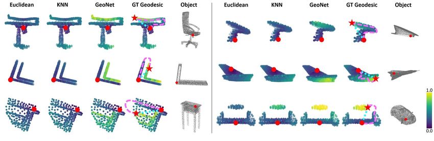
Figure 2. GeoNet: geodesic neighborhood estimation network.

cloud of non-rigid objects often consists of two steps: ex-       tances between points in the set χ. To demonstrate the ap-
tracting intrinsic features in geodesic space and applying        plicability of learned deep geodesic-aware representations
a classifier (e.g. SVM, MLP, etc.). Some commonly                 from GeoNet, we test our approach on typical tasks that
used features include wave kernel signatures [3], heat ker-       require understandings of the underlying surface topology,
nel signatures [31], spectral graph wavelet signatures [25],      including point cloud upsampling, surface normal estima-
Shape-DNA [29], etc. For example [24] uses geodesic mo-           tion, mesh reconstruction, and non-rigid shape classifica-
ments and stacked sparse autoencoders to classify non-rigid       tion. To this end, we leverage the existing state-of-the-
shapes, such as cat, horse, spider, etc. The geodesic mo-         art network architectures designed for the aforementioned
ments are feature vectors derived from the integral of the        problems. Specifically, we choose PU-Net as the base-
geodesic distance on a shape, while stacked sparse autoen-        line network for point upsampling and PointNet++ for other
coders are deep neural networks consisting of multiple lay-       tasks. The proposed geodesic fusion methods, called PU-
ers of sparse autoencoders. However, the above methods            Net fusion (PUF) and PointNet++ fusion (POF), integrate
all require knowing graph-based data, which is not avail-         GeoNet with the baseline or backbone models to conduct
able from widely used sensors (e.g. depth camera, Lidar,          geodesic-aware point set analysis.
etc.) for 3D data acquisition. Though PointNet++ [28] is
able to directly ingest a point cloud and conduct classifica-     3.3. Geodesic Neighborhood Estimation
tion, it is not designed to model the geodesic topology of
non-rigid shapes and thus its performance is inferior to tra-        As illustrated in Fig. 2, GeoNet consists of two modules:
ditional two-step methods which heavily reply on the offline      an autoencoder that extracts a feature vector ψ(xi ) for each
computed intrinsic surface features.                              point xi ∈ χ and a GM layer that acts as a learned geodesic
                                                                  kernel function for estimating Gr (xi ) using the latent fea-
3. Method                                                         tures.
3.1. Problem Statement                                               Feature Extraction. We use a variant of PointNet++,
                                                                  which is a point set based hierarchical and multi-scale func-
   χ = {xi } denotes a point set with xi ∈ Rd and                 tion, for feature extraction. It maps an input point set χ
i = 1, . . . , N . Although the problem and the method de-        to a feature set {ϕ(xi )|xi ∈ χ e} where ϕ(xi ) ∈ R3+C is
                                                                                                                            e

veloped are general, we focus on the case d = 3 using             a concatenation of the xyz coordinates and the C    e dimen-
only Euclidean coordinates as input. A neighborhood sub-          sional embedding of xi , and χ e is a sampled subset of χ by
set within radius r from a point xi is denoted Br (xi ) =         farthest-point sampling. To recover features {ψ(xi )} for the
{xj |dE (xi , xj ) ≤ r} where dE (xi , xj ) ∈ R is the Eu-        point cloud χ, we use a decoder with skip connections. The
clidean (embedding) distance between xi and xj . The cardi-       decoder consists of recursively applied tri-linear feature in-
nality of Br (xi ) is K. The corresponding geodesic distance      terpolators, shared fully connected (FC) layers, ReLU and
set around xi is called Gr (xi ) = {gij = dG (xi , xj )|xj ∈      Batch Normalization. The resulting (N, 3 + C) tensor is
Br (xi )} where dG ∈ R means the geodesic distance. Our           then fed into the GM layer for geodesic neighborhood esti-
goal is to learn a function f : xi 7→ Gr (xi ) that maps          mation.
each point to (an approximation of) the geodesic distance
                                                                     Geodesic Matching. We group the latent features ψ(xi )
set Gr (xi ) around it.
                                                                  into neighborhood feature sets Frl (xi ) = {ψ(xj )|xj ∈
                                                                  Brl (xi )}, under multiple radius scales rl . At each scale
3.2. Method
                                                                  rl we set a maximum number of neighborhood points Kl ,
   We introduce GeoNet, a network trained to learn the            and thus produce a tensor of dimension (N, Kl , 3+C). The
function f defined above. It consists of an autoencoder           grouped features, together with the latent features, are sent
with skip connections, followed by a multi-scale Geodesic         to a geodesic matching module, where ψ(xi ) is concate-
Matching (GM) layer, leveraging latent space features             nated with ψ(xj ) for every xj ∈ Brl (xi ). The resulting
{ψ(xi )} ⊆ R3+C of the point set. GeoNet is trained               feature ξij ∈ R3+2C becomes the input to a set of shared
in a supervised manner using ground truth geodesic dis-           FC layers with ReLU, Batch Normalization and Dropout.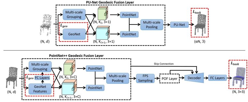
Figure 3. PU-Net (top) and PointNet++ (bottom) geodesic fusion architectures.

As demonstrated in [15], the multilayer perceptron (MLP)              (N, Kl , d + 1) fused tensor is fed to a PointNet to generate
acts as a kernel function that maps ξij to an approxima-              a (N, Cl ) feature tensor which will be stacked with features
tion of the geodesic distance, ĝij . Finally, the GM layer           from other neighborhood scales. The remaining layers are
yields Grl (xi ) for each point of thePinput point cloud χ. We        from PU-Net. As indicated by the red rectangles in Fig. 3,
use a multi-scale L1 loss Lgeo = l Lgeol to compare the               the total loss has two weighted terms:
ground truth geodesic distances to their estimates:

                                                                                              L = Lgeo + λLtask                            (2)
                   X        X           |gij − ĝ(xi , xj )|
         Lgeol =                                               (1)    where Lgeo is for GeoNet training (1), λ is a weight and
                   xi ∈χ xj ∈Br (xi )
                                              N Kl
                               l                                      Ltask , in general, is the loss for the current task that we are
                                                                      targeting. In this case, the goal is point cloud upsampling:
                                                                      Ltask = Lup (θ) where θ indicates network parameters.
3.4. Geodesic Fusion
                                                                      PUF upsampling takes a randomly distributed sparse point
    To demonstrate how the learned geodesic representations           set χ as input and generates a uniformly distributed dense
can be used for point set analysis, we propose fusion meth-           point cloud P̂ ⊆ R3 . The upsampling factor is α = |P       |
                                                                                                                                |χ| :
ods based on the state-of-the-art (SOTA) network archi-
tectures for different tasks. For example, PU-Net is the                                                                               2
SOTA upsampling method and thus we propose PUF that                       Lup (θ) = LEM D (P, P̂ ) + λ1 Lrep (P̂ ) + λ2 kθk                (3)
uses PU-Net as the baseline network to conduct geodesic
                                                                      in which the first term is the Earth Mover Distance (EMD)
fusion for point cloud upsampling. With connectivity infor-
                                                                      between the upsampled point set P̂ and the ground truth
mation provided by the estimated geodesic neighborhoods,
                                                                      dense point cloud P :
our geodesic-fused upsampling network can better recover
topological details, such as curves and sharp structures, than                                                 X                   2
PU-Net. We also present POF leveraging PointNet++ as the                      LEM D (P, P̂ ) = min                     kpi − φ(pi )k
                                                                                                    φ:P̂ →P                                (4)
fusion backbone, and demonstrate its effectiveness on both                                                    pi ∈P̂
geometric and semantic tasks where PointNet++ shows the
state-of-the-art performance.                                         where φ : P̂ → P indicates a bijection mapping.
    PU-Net Geodesic Fusion. A PUF layer, as illustrated                  The second term in (3) is a repulsion loss which pro-
in Fig. 3 (top), takes a (N, d) point set as input and sends          motes a uniform spatial distribution for P̂ by penalizing
it into two branches: one is a multi-scale Euclidean group-           close point pairs:
ing layer, and the other is GeoNet. At each neighborhood
scale rl , the grouped point set Brl (xi ) is fused with the es-                         X X
timated geodesic neighborhood Grl (xi ) to yield Srl (xi ) =              Lrep (P̂ ) =                   η(kpi − pj k)ω(kpi − pj k)
                                                                                                                                           (5)
{(xj , gij )|xj ∈ Brl (xi )} with (xj , gij ) ∈ Rd+1 . Then the                          pi ∈P̂ pj ∈P
                                                                                                    ei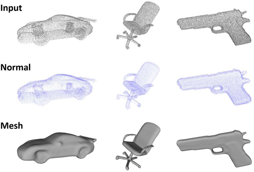
Figure 4. Representative results of geodesic neighborhood estimation. Red dots indicate the reference point and stars represent target points
selected for the purpose of illustration. Points in dark-purple are closer to the reference point than those in bright-yellow. Shortest paths
between the reference point and the target point in euclidean space are colored in sky-blue. Topology-based geodesic paths are in pink.

                    K-3      K-6     K-12      Euc     GeoNet                PointNet++ Geodesic Fusion. Fig. 3 (bottom) illus-
         r 6 0.1    8.75     8.97     9.04     9.06      5.67            trates the PointNet++ based fusion pipeline. Due to task
   v1    r 6 0.2   16.22    17.33    17.90    18.16      9.25            as well as architecture differences between PU-Net and
         r 6 0.4   15.15    16.80    17.88    18.95      9.75
                                                                         PointNet++, we make following changes to PUF to de-
         r 6 0.1   11.71    11.49    11.55    11.57      7.06            sign a suitable fusion strategy that leverages PointNet++.
   v2    r 6 0.2   19.22    17.76    18.28    18.56      9.74
                                                                         First, for multi-scale grouping, we use the learned geodesic
         r 6 0.4   21.03    17.19    18.20    19.44     10.04
                                                                         neighborhoods Ĝr (xi ) instead of Euclidean ones. Geodesic
         r 6 0.1   13.28    14.23    14.62    14.78     10.86
                                                                         grouping brings attention to the underlying surfaces as well
   v3    r 6 0.2   14.85    17.27    18.54    19.49     13.61
         r 6 0.4   13.48    16.10    17.72    19.68     14.73            as structures of the point cloud. Second, while the PUF
                                                                         layer fuses estimated Ĝr (xi ) = {ĝij = dˆG (xi , xj )|xj ∈
Table 1. Neighborhood geodesic distance estimation MSE (x100)            Br (xi )}, where ĝij ∈ R, of each neighborhood point set
on the heldout ShapeNet training-category samples. We com-               Br (xi ) into the backbone network, the POF layer uses the
pare with KNN-Graph based shortest path methods under different
                                                                         latent geodesic-aware features ξeij ∈ RC extracted from the
                                                                                                                    e
choices of K values. Euc represents the difference between Eu-
clidean distance and geodesic distance. MSE(s) are reported under        second-to-last FC layer in GeoNet. Namely, ξeij is an inter-
multiple radius ranges r. v1 takes uniformly distributed point sets      mediate high-dimensional feature vector from ξij to ĝij via
with 512 points as input, and v2 uses randomly distributed point         FC layers, and therefore it is better informed of the intrin-
clouds. v3 is tested using point clouds that have 2048 uniformly         sic point cloud topology. Third, in PointNet++ fusion we
distributed points.                                                      apply the POF layer in a hierarchical manner, leveraging
                                                                         farthest-point sampling. Thus, the learned features encode
                    K-3      K-6     K-12      Euc     GeoNet            both local and global structural information of the point set.
         r 6 0.1    8.81     9.01     9.05     9.06      7.52            The total loss for POF also has two parts: One is for GeoNet
   v1
         r 6 0.2   11.84    12.88    13.49    13.75     11.44            training and the other is for the task-at-hand. We experiment
         r 6 0.1   10.52    10.21    10.25    10.26      8.94            on representative tasks that can benefit from understandings
   v2
         r 6 0.2   15.02    12.99    13.59    13.86     11.69            of the topological surface attributes. We use the L1 error for
         r 6 0.1   11.82    12.39    12.65    12.75     10.88            point cloud normal estimation:
   v3
         r 6 0.2   11.80    12.84    13.55    14.50     12.26

Table 2. Geodesic neighborhood estimation MSE (x100) on the                                                     (j)
leftout ShapeNet categories. v1 takes uniformly distributed point                                   3
                                                                                                   XX ni − n̂(xi )(j)
sets with 512 points as input, and v2 uses randomly distributed                      Lnormal =                                           (6)
                                                                                                  xi ∈χ j=1
                                                                                                                      3N
point clouds. v3 is tested using point clouds that have 2048 uni-
formly distributed points.
                                                                         in which ni ∈ R3 is the ground truth unit normal vector of
                                                                         xi , and n̂(xi ) ∈ R3 is the estimated normal. We then use
where Pei is a set of k-nearest neighbors of pi , η(r) = −r              the normal estimation to generate mesh via Poisson surface
                                                2  2
penalizes close pairs (pi , pj ), and ω(r) = e−r /h is a fast-           reconstruction [21]. To classify point clouds of non-rigid
decaying weight function with some constant h [18, 23].                  objects, we use cross-entropy loss: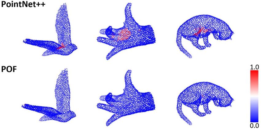
Figure 5. Point cloud upsampling comparisons with PU-Net. The input point clouds have 512 points with random distributions and the
upsampled point clouds have 2048 points. Red insets show details of the corresponding dashed region in the reconstruction.

                            S
                            X
                 Lcls = −         yc log(pc (χ))             (7)
                            c=1

where S is the number of non-rigid object categories, and c
is class label; yc ∈ {0, 1} is a binary indicator, which takes
value 1 if class label c is ground truth for the input point set.
pc (χ) ∈ R is the predicted probability w.r.t. class c of the
input point set.
                                                                    Figure 6. Top-k mean square error (MSE) of upsampled points that
3.5. Implementation                                                 have large errors, for both the heldout training-category samples
                                                                    (red) and the leftout ShapeNet categories (green).
   For GeoNet training, the multiscale loss Lgeol is en-
forced at three radius ranges: 0.1, 0.2 and 0.4. We use                                             MSE     EMD      CD
Adam [22] with learning rate 0.001 and batchsize 3 for 8                                 PU-Net      7.14    8.06    2.72
epochs. To train the geodesic fusion networks, we set the                     Training
                                                                                          PUF        6.23    7.62    2.46
task term weight λ as 1, and use Adam with learning rate                                 PU-Net     12.38   11.43    3.98
0.0001 and batchsize 2 for around 300 to 1500 epochs de-                       Leftout
                                                                                          PUF        9.55    8.90    3.27
pending on the task and the dataset. Source code in Tensor-
flow will be made available upon completion of the anony-           Table 3. Point cloud upsampling results on both the heldout
mous review process.                                                training-category samples and the unseen ShapeNet categories.
                                                                    MSE(s) (x10000) are scaled for better visualization.
4. Experiments
    We put GeoNet to the test by estimating point cloud             scales r w.r.t. xi ∈ χ. GeoNet demonstrates consistent
geodesic neighborhoods. To demonstrate the applicabil-              improvement over the baselines. Representative results are
ity of learned deep geodesic-aware representations, we also         visualized in Fig. 4. Our method captures various topologi-
conduct experiments on down-stream point cloud tasks such           cal patterns, such as curved surfaces, layered structures, in-
as point upsampling, normal estimation, mesh reconstruc-            ner/outer parts, etc.
tion and non-rigid shape classification.                               Generality. We test GeoNet’s robustness under different
                                                                    point set distributions and sizes. In Tab. 1 (v2) we use point
4.1. Geodesic Neighborhood Estimation
                                                                    clouds with 512 randomly distributed points as input. We
   In Tab. 1 (v1) we show geodesic distance set, Gr (xi ),          also test on dense point sets that contain 2048 uniformly
estimation results on the ShapeNet dataset [5] using point          distributed points in Tab. 1 (v3). Our results are robust to
clouds with 512 uniformly distributed points. Mean-                 different point set distributions as well as sizes. To show the
squared errors (MSE) are reported under multiple radius             generalization performance, in Tab. 2 we report results on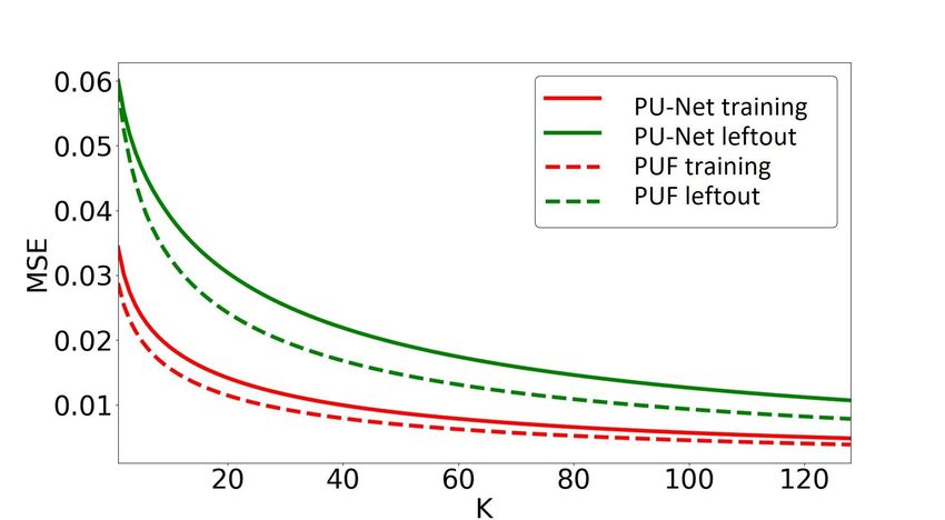
Figure 7. Mesh reconstruction results on the Shrec15 (left) and the ShapeNet (right) datasets using the estimated normal by PointNet++
and our method POF. GT presents mesh reconstructed via the ground truth normal. We also visualize POF normal estimation in the fourth
and the last columns.

                                                                      4.2. Point Cloud Upsampling
                                                                         We test PUF on point cloud upsampling and present re-
                                                                      sults in Tab. 3. We compare against the state-of-the-art point
                                                                      set upsampling method PU-Net on three metrics: MSE,
                                                                      EMD as well as the Chamfer Distance (CD). Our method
                                                                      outperforms the baseline under all metrics by 9.25% av-
                                                                      erage improvement on the heldout training-category sam-
                                                                      ples. Since geodesic neighborhoods are better informed of
Figure 8. Point set normal estimation errors. Blue indicates small    the underlying point set topology than Euclidean ones, PUF
errors and red is for large ones.                                     upsampling produces less outliers and recovers more details
                                                                      in Fig. 5, such as curves and sharp structures.
                                                                         Generality. To analyze outlier robustness (i.e. points
                6 2.5◦        6 5◦           6 10◦         6 15◦
                                                                      with large reconstruction errors), we plot top-k MSE in
    PCA        6.16±0.01   14.85±0.02     27.16±0.17    34.17±0.28
                                                                      Fig. 6. Our method generates fewer outliers on both the
 PointNet++   12.81±0.18   33.37±0.92     61.58±2.02    75.49±1.95
    POF       16.26±0.30   39.02±1.09     66.98±1.46    79.66±1.21    heldout training-category samples and the unseen cate-
                                                                      gories. We also report quantitative results on the leftout
Table 4. Point cloud normal estimation accuracy (%) on the            categories in Tab. 3. Again, PUF significantly surpasses the
Shrec15 dataset under multiple angle thresholds.                      state-of-the-art upsampling method PU-Net under three dif-
                                                                      ferent evaluation metrics.
                            6 2.5◦       6 5◦   6 10◦     6 15◦       4.3. Normal Estimation and Mesh Reconstruction
                 PCA          5.33      10.11   18.52     24.82
   Training   PointNet++     30.68      43.19   55.91     62.30          For normal estimation we apply PointNet++ geodesic fu-
                 POF         32.04      45.02   57.52     63.62       sion, POF, then we conduct Poisson mesh reconstruction
                 PCA          5.24      10.59   18.99     25.17       leveraging the estimated normals. Quantitative results for
   Leftout    PointNet++     17.35      28.82   43.26     51.17       normal estimation on the Shrec15 dataset and the ShapeNet
                 POF         19.13      31.83   46.22     53.78       dataset are given in Tab. 4 and Tab. 5, respectively. We com-
                                                                      pare our method with the traditional PCA algorithm as well
Table 5. Point cloud normal estimation accuracy (%) on the
ShapeNet dataset for both heldout training-category samples and       as the state-of-the-art deep learning method PointNet++.
leftout categories.                                                   Our results outperform the baselines by around 10% rela-
                                                                      tive improvement. In Fig. 8, we visualize typical normal
                                                                      estimation errors, showing that PointNet++ usually fails at
                                                                      high-curvature and complex-surface regions. For further ev-
the leftout ShapeNet categories. Our method performs bet-             idence, we visualize Poisson mesh reconstruction in Fig. 7
ter on unseen categories, while KNN-Graph based shortest              using the estimated normals.
path approaches suffer from point set distribution random-               Generality. In Tab. 5 we evaluate normal estimation per-
ness, density changes and unsuitable choices of K values.             formance on the leftout ShapeNet categories. Our method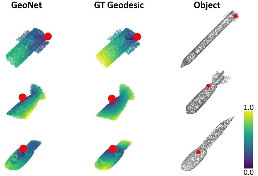
Figure 9. Normal estimation and Poisson mesh reconstruction re-   Figure 10. Failure cases of geodesic neighborhood estimation for
sults by POF using dense point clouds with 8192 points.           stick-shaped objects (e.g. rocket, knife, etc.) which have large
                                                                  ratios between length and width/height. Red dots indicate the ref-
                         Input feature      Accuracy (%)          erence point. Points in dark-purple are closer to the reference point
          PointNet++         XYZ               73.56              than those in bright-yellow.
             POF             XYZ               94.67
           DeepGM      Intrinsic features      93.03

Table 6. Point cloud classification of non-rigid shapes on the    while PointNet++ decreases by up to 15.20%.
Shrec15 dataset.

                            Gaussian Noise Level                  4.5. Failure Modes
                    0.8%    0.9% 1.0% 1.1%            1.2%
       PointNet++   70.54   69.27 67.83 65.66         62.38           Failure cases of geodesic neighborhood estimation are
          POF       91.89   90.93 89.40 87.72         84.98
                                                                  shown in Fig. 10. Due to large ratios between length and
Table 7. Noisy point clouds classification accuracy (%). We add   width/height, after normalizing a stick-shaped object (e.g.
Gaussian noise of 0.8% to 1.2% of unit ball radius.               rocket, knife, etc.) into a unit ball we need high precision
                                                                  small values to represent its point-pair geodesic distance
                                                                  along the width/height sides. Since stick-shaped objects
has higher accuracy over competing methods under multi-           like rocket and knife only take up a small portion of the
ple angle thresholds. Though trained with point clouds of         training data, GeoNet tends to make mistakes for heldout
2048 points, POF is also tested on denser input. In Fig. 9        samples from these categories at inference time. We have
we take point clouds with 8192 points as input, and visual-       not found additional failure cases, and quantitative improve-
ize the normal estimation and mesh reconstruction results,        ments continue to take effect due to rich surface-based topo-
which shows that our method generalizes to dense point            logical information learned during the geodesic-supervised
clouds without re-training and produces fine-scaled mesh.         training process.
4.4. Non-rigid Shape Classification
   Results of non-rigid shape classification are reported in      5. Conclusion
Tab. 6. While POF and PointNet++ only take point cloud-
based xyz Euclidean coordinates as input, DeepGM re-                 We have presented GeoNet, a novel deep learning archi-
quires offline computed intrinsic features from mesh data in      tecture to learn the geodesic space-based topological struc-
the ground truth geodesic metric space. Though using less         ture within point clouds. The training process is super-
informative data, our method has higher classification ac-        vised by the ground truth geodesic distance and therefore
curacy than other methods, which further demonstrates that        the learned representations reflect the intrinsic structure of
the proposed geodesic fusion architecture, POF, is suitable       the underlying point set surfaces. To demonstrate the ap-
for solving tasks that require understandings of the underly-     plicability of such a topology estimation network, we also
ing point cloud surface attributes.                               propose fusion methods to incorporate GeoNet into com-
   Generality. We add Gaussian noise of different lev-            putational schemes that involve the standard backbone ar-
els to the input and conduct noisy point clouds classifica-       chitectures for point cloud analysis. Our method is tested
tion. Comparisons are shown in Tab. 7. POF outperforms            on both geometric and semantic tasks and outperforms the
PointNet++ under several noise levels. Our method also            state-of-the-art methods, including point upsampling, nor-
demonstrates better noise robustness. It shows a 10.24%           mal estimation, mesh reconstruction and non-rigid shape
decrease in relative accuracy at the maximum noise level,         classification.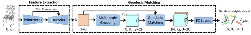
References                                                           [16] X. Han, Z. Li, H. Huang, E. Kalogerakis, and Y. Yu. High-
                                                                          resolution shape completion using deep neural networks for
 [1] M. Alexa, J. Behr, D. Cohen-Or, S. Fleishman, D. Levin,              global structure and local geometry inference. In Proceed-
     and C. T. Silva. Computing and rendering point set surfaces.         ings of IEEE International Conference on Computer Vision
     IEEE Transactions on visualization and computer graphics,            (ICCV), 2017.
     9(1):3–15, 2003.
                                                                     [17] H. Hoppe, T. DeRose, T. Duchamp, J. McDonald, and
 [2] N. Amenta and M. Bern. Surface reconstruction by voronoi             W. Stuetzle. Surface reconstruction from unorganized points,
     filtering. Discrete & Computational Geometry, 22(4):481–             volume 26. ACM, 1992.
     504, 1999.
                                                                     [18] H. Huang, D. Li, H. Zhang, U. Ascher, and D. Cohen-Or.
 [3] M. Aubry, U. Schlickewei, and D. Cremers. The wave kernel            Consolidation of unorganized point clouds for surface recon-
     signature: A quantum mechanical approach to shape analy-             struction. ACM transactions on graphics (TOG), 28(5):176,
     sis. In Computer Vision Workshops (ICCV Workshops), 2011             2009.
     IEEE International Conference on, pages 1626–1633. IEEE,
                                                                     [19] D. B. Johnson. Efficient algorithms for shortest paths in
     2011.
                                                                          sparse networks. Journal of the ACM (JACM), 24(1):1–13,
 [4] F. Cazals and M. Pouget. Estimating differential quantities
                                                                          1977.
     using polynomial fitting of osculating jets. Computer Aided
                                                                     [20] I. Jolliffe. Principal component analysis. In International en-
     Geometric Design, 22(2):121–146, 2005.
                                                                          cyclopedia of statistical science, pages 1094–1096. Springer,
 [5] A. X. Chang, T. Funkhouser, L. Guibas, P. Hanrahan,
                                                                          2011.
     Q. Huang, Z. Li, S. Savarese, M. Savva, S. Song, H. Su,
                                                                     [21] M. Kazhdan and H. Hoppe. Screened poisson surface recon-
     et al. Shapenet: An information-rich 3d model repository.
                                                                          struction. ACM Transactions on Graphics (ToG), 32(3):29,
     arXiv preprint arXiv:1512.03012, 2015.
                                                                          2013.
 [6] J. Chen and Y. Han. Shortest paths on a polyhedron. In Pro-
     ceedings of the sixth annual symposium on Computational         [22] D. P. Kingma and J. Ba. Adam: A method for stochastic
     geometry, pages 360–369. ACM, 1990.                                  optimization. arXiv preprint arXiv:1412.6980, 2014.
 [7] K. Crane, C. Weischedel, and M. Wardetzky. Geodesics in         [23] Y. Lipman, D. Cohen-Or, D. Levin, and H. Tal-Ezer.
     heat: A new approach to computing distance based on heat             Parameterization-free projection for geometry reconstruc-
     flow. ACM Transactions on Graphics (TOG), 32(5):152,                 tion. ACM Transactions on Graphics (TOG), 26(3):22, 2007.
     2013.                                                           [24] L. Luciano and A. B. Hamza. Deep learning with geodesic
 [8] A. Dai, C. R. Qi, and M. Nießner. Shape completion us-               moments for 3d shape classification. Pattern Recognition
     ing 3d-encoder-predictor cnns and shape synthesis. In Proc.          Letters, 105:182–190, 2018.
     IEEE Conf. on Computer Vision and Pattern Recognition           [25] M. Masoumi, C. Li, and A. B. Hamza. A spectral graph
     (CVPR), volume 3, 2017.                                              wavelet approach for nonrigid 3d shape retrieval. Pattern
 [9] M. Defferrard, X. Bresson, and P. Vandergheynst. Convolu-            Recognition Letters, 83:339–348, 2016.
     tional neural networks on graphs with fast localized spectral   [26] J. S. Mitchell, D. M. Mount, and C. H. Papadimitriou. The
     filtering. In Advances in Neural Information Processing Sys-         discrete geodesic problem. SIAM Journal on Computing,
     tems, pages 3844–3852, 2016.                                         16(4):647–668, 1987.
[10] E. W. Dijkstra. A note on two problems in connexion with        [27] C. R. Qi, H. Su, K. Mo, and L. J. Guibas. Pointnet: Deep
     graphs. Numer. Math., 1(1):269–271, Dec. 1959.                       learning on point sets for 3d classification and segmentation.
[11] R. W. Floyd. Algorithm 97: shortest path. Communications             Proc. Computer Vision and Pattern Recognition (CVPR),
     of the ACM, 5(6):345, 1962.                                          IEEE, 1(2):4, 2017.
[12] M. Garland and P. S. Heckbert. Surface simplification us-       [28] C. R. Qi, L. Yi, H. Su, and L. J. Guibas. Pointnet++: Deep hi-
     ing quadric error metrics. In Proceedings of the 24th an-            erarchical feature learning on point sets in a metric space. In
     nual conference on Computer graphics and interactive tech-           Advances in Neural Information Processing Systems, pages
     niques, pages 209–216. ACM Press/Addison-Wesley Pub-                 5099–5108, 2017.
     lishing Co., 1997.                                              [29] M. Reuter, F.-E. Wolter, and N. Peinecke. Laplace–beltrami
[13] G. Guennebaud and M. Gross. Algebraic point set sur-                 spectra as shape-dnaof surfaces and solids. Computer-Aided
     faces. In ACM Transactions on Graphics (TOG), volume 26,             Design, 38(4):342–366, 2006.
     page 23. ACM, 2007.                                             [30] M. Sharir and A. Schorr. On shortest paths in polyhedral
[14] P. Guerrero, Y. Kleiman, M. Ovsjanikov, and N. J. Mitra.             spaces. SIAM Journal on Computing, 15(1):193–215, 1986.
     Pcpnet learning local shape properties from raw point clouds.   [31] J. Sun, M. Ovsjanikov, and L. Guibas. A concise and prov-
     In Computer Graphics Forum, volume 37, pages 75–85. Wi-              ably informative multi-scale signature based on heat diffu-
     ley Online Library, 2018.                                            sion. In Computer graphics forum, volume 28, pages 1383–
[15] X. Han, T. Leung, Y. Jia, R. Sukthankar, and A. C. Berg.             1392. Wiley Online Library, 2009.
     Matchnet: Unifying feature and metric learning for patch-       [32] V. Surazhsky, T. Surazhsky, D. Kirsanov, S. J. Gortler, and
     based matching. In Proceedings of the IEEE Conference                H. Hoppe. Fast exact and approximate geodesics on meshes.
     on Computer Vision and Pattern Recognition, pages 3279–              In ACM transactions on graphics (TOG), volume 24, pages
     3286, 2015.                                                          553–560. Acm, 2005.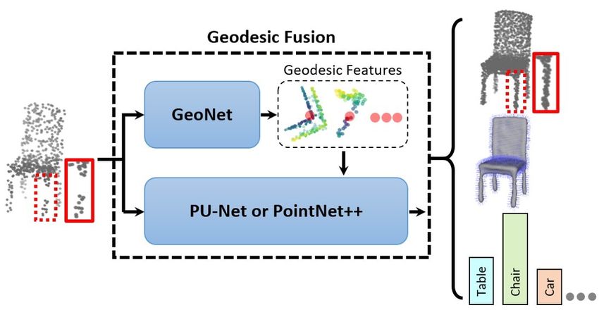
[33] J. Wu, C. Zhang, T. Xue, B. Freeman, and J. Tenenbaum.
     Learning a probabilistic latent space of object shapes via 3d
     generative-adversarial modeling. In Advances in Neural In-
     formation Processing Systems, pages 82–90, 2016.
[34] Z. Wu, S. Song, A. Khosla, F. Yu, L. Zhang, X. Tang, and
     J. Xiao. 3d shapenets: A deep representation for volumetric
     shapes. In Proceedings of the IEEE conference on computer
     vision and pattern recognition, pages 1912–1920, 2015.
[35] S.-Q. Xin and G.-J. Wang. Improving chen and han’s algo-
     rithm on the discrete geodesic problem. ACM Transactions
     on Graphics (TOG), 28(4):104, 2009.
[36] L. Yi, H. Su, X. Guo, and L. J. Guibas. Syncspeccnn: Syn-
     chronized spectral cnn for 3d shape segmentation. In CVPR,
     pages 6584–6592, 2017.
[37] L. Yu, X. Li, C.-W. Fu, D. Cohen-Or, and P.-A. Heng. Pu-
     net: Point cloud upsampling network. In Proceedings of the
     IEEE Conference on Computer Vision and Pattern Recogni-
     tion, pages 2790–2799, 2018.
You can also read