Global Temperature in 2017 - Columbia University
←
→
Page content transcription
If your browser does not render page correctly, please read the page content below
Global Temperature in 2017
18 January 2018
a a
James Hansen , Makiko Sato , Reto Ruedy b,c
Gavin A. Schmidt , Ken Lo , Avi Persinb,c
c b,c
Abstract. Global surface temperature in 2017 was the second highest in the period of
instrumental measurements in the Goddard Institute for Space Studies (GISS) analysis. Relative to
average temperature for 1880-1920, which we take as an appropriate estimate of “pre-industrial”
temperature, 2017 was +1.17°C (~2.1°F) warmer than in the 1880-1920 base period. The high 2017
temperature, unlike the record 2016 temperature, was obtained without any boost from tropical El
Niño warming.
Update of the GISS (Goddard Institute for Space Studies) global temperature analysis (GISTEMP) 1, 2
(Fig. 1), finds 2017 to be the second warmest year in the instrumental record. (More detail is available at
http://data.giss.nasa.gov/gistemp/ and http://www.columbia.edu/~mhs119/Temperature; figures here are
available from Makiko Sato on the latter web site.) A few figures are included below as an appendix.
We take 1880-1920 as baseline, i.e., as the zero-point for temperature anomalies, because it is the
earliest period with substantial global coverage of instrumental measurements and because it also has a
global mean temperature that should approximate “preindustrial” temperature 3.
We estimate current underlying temperature, excluding short-term variability via linear fit to the post-
1970 temperature (Fig. 1). The result is +1.07°C at the beginning of 2018 relative to 1880-1920.
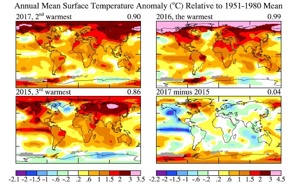
Figure 2 compares maps of global temperature anomalies of the past three years. The map in the
lower right is the difference between 2017 and 2015 temperatures, revealing that 2017 was notably
warmer than 2015 in the polar regions. This 2017-2015 difference map suggests the reason why some
temperature analyses report 2017 as the third warmest year, behind 2015 as well as 2016. Some analyses
include only area close to the points of actual observations in their ‘global’ analysis. The GISS analysis1
extrapolates observations as far as 1200 km from measurement points, thus covering practically the entire
globe. It has been shown, by sampling globally complete data with realistic temporal and spatial
variability, that this extrapolation procedure yields a more accurate estimate of annual global temperature
than global integration methods that restrict the area to regions very close to observed points. 4,1
Fig. 1. (a) Global surface temperatures relative to 1880-1920 based on GISTEMP data, which employs GHCN.v3
for meteorological stations, NOAA ERSST.v5 for sea surface temperature, and Antarctic research station data1.
a
Earth Institute, Columbia University, New York, NY
b
SciSpace LLC, New York, NY
c
NASA Goddard Institute for Space Studies, New York, NY
1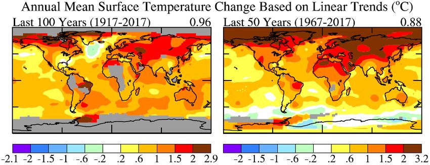
Fig. 2. Temperature anomalies in 2017, 2016 and 2015 relative to 1951-1980 base period. The lower right map
shows the difference between the 2017 and 2015 maps. We use the 1951-1980 base period for maps because of
more limited global data coverage in 1880-1920.

    Figure 3 compares the GISS analysis of global temperature change with the case in which the polar
regions, specifically regions poleward of 64 degrees latitude, are excluded from the analysis. With polar
regions excluded, 2017 becomes the third warmest year, and the ‘global’ warming relative to the base
period is reduced by almost a tenth of a degree Celsius. We do not mean to imply that other analyses
entirely exclude polar regions. Therefore we make a more specific test of the impact of omitted regions
by carrying out the GISS analysis with local measurements extrapolated only 250 km rather than 1200
km. Fig. A2 shows that this area limit also causes 2017 to be only the third warmest year.
    We conclude that 2017 probably was the second warmest year. However, the temperatures of 2015
and 2017 are so close that the difference is unimportant.
    Prospects for continued global temperature change are more interesting and important. The record
2016 temperature was abetted by the effects of both a strong El Niño and maximum warming from the
solar irradiance cycle (Fig. 4). Because of the ocean thermal inertia and decadal irradiance change, the
peak warming and cooling effects of solar maximum and minimum are delayed about two years after
irradiance extrema. The amplitude of the solar irradiance variation is smaller than the planetary energy

Fig. 3. Global temperature compared with the result for integration over the region from 64°N to 64°S, which covers
90% of Earth’s surface, excluding only polar regions.
                                                        2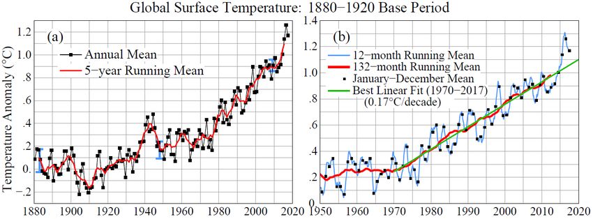
Fig. 4. Solar irradiance and sunspot number in the era of satellite data. Left scale is the energy passing
through an area perpendicular to Sun-Earth line. Averaged over Earth’s surface the absorbed solar energy
is ~240 W/m2, so the full amplitude of the measured solar variability is ~0.25 W/m2.

imbalance, which has grown to about +0.75 ± 0.25 W/m2 over the past several decades due to increasing
atmospheric greenhouse gases. 5,6 However, the solar variability is not negligible in comparison with the
energy imbalance that drives global temperature change. Therefore, because of the combination of the
strong 2016 El Niño and the phase of the solar cycle, it is plausible, if not likely, that the next 10 years of
global temperature change will leave an impression of a ‘global warming hiatus’.
    On the other hand, the 2017 global temperature remains stubbornly high, well above the trend line
(Fig. 1), despite cooler than average temperature in the tropical Pacific Niño 3.4 region (Fig. 5), which
usually provides an indication of the tropical Pacific effect on global temperature 7. Conceivably this
continued temperature excursion above the trend line is not a statistical fluke, but rather is associated with
climate forcings and/or feedbacks. The growth rate of greenhouse gas climate forcing has accelerated in
the past decade.3 There is also concern that polar climate feedbacks may accelerate. 8
    Therefore, temperature change during even the next few years is of interest, to determine whether a
significant excursion above the trend line is underway.

Fig. 5. Niño 3.4 and global temperature change during the past five years.

                                                        3
Appendix
Fig. A1. Global surface temperature relative to 1880-1920 based on GISTEMP data. (a) Annual and 5-year means
since 1880, (b) 12- and 132-month running means since 1970. Blue squares in (b) are calendar year (Jan-Dec)
means used to construct (a). Update of Fig. 2 in reference 3.
Fig. A2. Global surface temperature with extrapolation of data limited to 250 km from observations.
Fig. A3. Global temperature in the past 100 and past 50 years based on local linear trends.
4References
1
Hansen, J., R. Ruedy, M. Sato, and K. Lo, 2010: Global surface temperature change. Rev. Geophys., 48, RG4004,
doi:10.1029/2010RG000345.
2
The current GISS analysis employs NOAA ERSST.v5 for sea surface temperature, GHCN.v.3.3.0 for
meteorological stations, and Antarctic research station data, as described in reference 1.
3
Hansen, J., M. Sato, P. Kharecha, K. von Schuckmann, D.J. Beerling, J. Cao, S. Marcott, V. Masson-Delmotte,
M.J. Prather, E.J. Rohling, J. Shakun, P. Smith, A. Lacis, G. Russell, and R. Ruedy, 2017: Young people's burden:
Requirement of negative CO2 emissions. Earth Syst. Dynam., 8, 577-616, doi:10.5194/esd-8-577-2017.
4
Hansen, J.E., and S. Lebedeff, 1987: Global trends of measured surface air temperature. J. Geophys. Res., 92,
13345-13372, doi:10.1029/JD092iD11p13345.
5
von Schuckmann, K., M.D. Palmer, K.E. Trenberth, A. Cazenave, D. Chambers, N. Champollion, J. Hansen, S.A.
Josey, N. Loeb, P.-P. Mathieu, B. Meyssignac, M. Wild, 2016: An imperative to monitor Earth's energy imbalance
Nature Climate Change 6, 138-144, doi:10.1038/nclimate2876.
6
Hansen, J., M. Sato, P. Kharecha, and K. von Schuckmann, 2011: Earth's energy imbalance and implications.
Atmos. Chem. Phys., 11, 13421-13449, doi:10.5194/acp-11-13421-2011.
7
Philander, S.G., Our Affair with El Niño: How We Transformed an Enchanting Peruvian Current into a Global
Climate Hazard, Princeton Univ. Press, Princeton, NJ, 288 pp., 2006.
8
Sommerkorn, M. and Hassol, S.J., 2009: Arctic Climate Feedbacks: Global Implications, World Wildlife Fund
report, 98 pages, based on Sommerkorn M., Hamilton N. (eds.) 2008. Arctic Climate Impact Science – an update
since ACIA. http://assets.panda.org/downloads/arctic_climate_impact_science_1.pdf
5You can also read