Go-Explore: a New Approach for Hard-Exploration Problems
←
→
Page content transcription
If your browser does not render page correctly, please read the page content below
Go-Explore: a New Approach for Hard-Exploration
                                                                Problems

                                             Adrien Ecoffet      Joost Huizinga  Joel Lehman       Kenneth O. Stanley*               Jeff Clune*
                                                                                  Uber AI Labs
                                                                             San Francisco, CA 94103
                                                                   adrienecoffet,joost.hui,jclune@gmail.com
arXiv:1901.10995v4 [cs.LG] 26 Feb 2021

                                                                                *Co-senior authors

                                         Authors’ note: We recommend reading (and citing) our updated paper, “First return, then explore”:
                                         Ecoffet, A., Huizinga, J., Lehman, J., Stanley, K.O. and Clune, J. First return, then explore. Nature
                                         590, 580–586 (2021). https://doi.org/10.1038/s41586-020-03157-9
                                         It can be found at https://tinyurl.com/Go-Explore-Nature.

                                                                                       Abstract
                                                   A grand challenge in reinforcement learning is intelligent exploration, especially
                                                   when rewards are sparse or deceptive. Two Atari games serve as benchmarks for
                                                   such hard-exploration domains: Montezuma’s Revenge and Pitfall. On both games,
                                                   current RL algorithms perform poorly, even those with intrinsic motivation, which
                                                   is the dominant method to encourage exploration and improve performance on hard-
                                                   exploration domains. To address this shortfall, we introduce a new algorithm called
                                                   Go-Explore. It exploits the following principles: (1) remember states that have
                                                   previously been visited, (2) first return to a promising state (without exploration),
                                                   then explore from it, and (3) solve simulated environments through exploiting any
                                                   available means (including by introducing determinism), then robustify (create a
                                                   policy that can reliably perform the solution) via imitation learning. The combined
                                                   effect of these principles generates dramatic performance improvements on hard-
                                                   exploration problems. On Montezuma’s Revenge, without being provided any
                                                   domain knowledge, Go-Explore scores over 43,000 points, almost 4 times the
                                                   previous state of the art. Go-Explore can also easily harness human-provided
                                                   domain knowledge, and when augmented with it Go-Explore scores a mean of
                                                   over 650,000 points on Montezuma’s Revenge. Its max performance of 18 million
                                                   surpasses the human world record by an order of magnitude, thus meeting even
                                                   the strictest definition of “superhuman” performance. On Pitfall, Go-Explore with
                                                   domain knowledge is the first algorithm to score above zero. Its mean performance
                                                   of almost 60,000 points also exceeds expert human performance. Because Go-
                                                   Explore can produce many high-performing demonstrations automatically and
                                                   cheaply, it also outperforms previous imitation learning work in which the solution
                                                   was provided in the form of a human demonstration. Go-Explore opens up many
                                                   new research directions into improving it and weaving its insights into current RL
                                                   algorithms. It may also enable progress on previously unsolvable hard-exploration
                                                   problems in a variety of domains, especially the many that often harness a simulator
                                                   during training (e.g. robotics).

                                         1     Introduction
                                         Reinforcement learning (RL) has experienced significant progress in recent years, achieving super-
                                         human performance in board games such as Go [1, 2] and in classic video games such as Atari [3].
                                         However, this progress obscures some of the deep unmet challenges in scaling RL to complex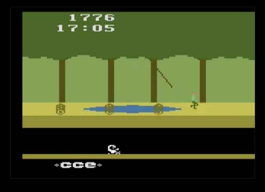
real-world domains. In particular, many important tasks require effective exploration to be solved, i.e.
to explore and learn about the world even when rewards are sparse or deceptive. In sparse-reward
problems, precise sequences of many (e.g. hundreds or more) actions must be taken between ob-
taining rewards. Deceptive-reward problems are even harder, because instead of feedback rarely
being provided, the reward function actually provides misleading feedback for reaching the overall
global objective, which can lead to getting stuck on local optima. Both sparse and deceptive reward
problems constitute “hard-exploration” problems, and classic RL algorithms perform poorly on
them [4]. Unfortunately, most challenging real-world problems are also hard-exploration problems.
That is because we often desire to provide abstract goals (e.g. “find survivors and tell us their location,”
or “turn off the valve to the leaking pipe in the reactor”), and such reward functions do not provide
detailed guidance on how to solve the problem (sparsity) while also often creating unintended local
optima (deception) [5–8].
For example, in the case of finding survivors in a disaster area, survivors will be few and far between,
thus introducing sparsity. Even worse, if we also instruct the robot to minimize damage to itself,
this additional reward signal may actively teach the robot not to explore the environment, because
exploration is initially much more likely to result in damage than it is to result in finding a survivor.
This seemingly sensible additional objective thus introduces deception on top of the already sparse
reward problem.
To address these challenges, this paper introduces Go-Explore, a new algorithm for hard-exploration
problems that dramatically improves state-of-the-art performance in two classic hard-exploration
benchmarks: the Atari games Montezuma’s Revenge and Pitfall.
Prior to Go-Explore, the typical approach to sparse reward problems has been intrinsic motivation
(IM) [4, 9–11], which supplies the RL agent with intrinsic rewards (IRs) that encourage exploration
(augmenting or replacing extrinsic reward that comes from the environment). IM is often motivated by
psychological concepts such as curiosity [12, 13] or novelty-seeking [7, 14], which play a role in how
humans explore and learn. While IM has produced exciting progress in sparse reward problems, in
many domains IM approaches are still far from fully solving the problem, including on Montezuma’s
Revenge and Pitfall. We hypothesize that, amongst other issues, such failures stem from two root
causes that we call detachment and derailment.
Detachment is the idea that an agent driven by IM could become detached from the frontiers of
high intrinsic reward (IR). To understand detachment, we must first consider that intrinsic reward
is nearly always a consumable resource: a curious agent is curious about states to the extent that it
has not often visited them (similar arguments apply for surprise, novelty, or prediction-error seeking
agents [4, 14–16]). If an agent discovers multiple areas of the state space that produce high IR, its
policy may in the short term focus on one such area. After exhausting some of the IR offered by that
area, the policy may by chance begin consuming IR in another area. Once it has exhausted that IR, it
is difficult for it to rediscover the frontier it detached from in the initial area, because it has already
consumed the IR that led to that frontier (Fig. 1), and it likely will not remember how to return to
that frontier due to catastrophic forgetting [17–20]. Each time this process occurs, a potential avenue
of exploration can be lost, or at least be difficult to rediscover. In the worst case, there may be a
dearth of remaining IR near the areas of state space visited by the current policy (even though much
IR might remain elsewhere), and therefore no learning signal remains to guide the agent to further
explore in an effective and informed way. One could slowly add intrinsic rewards back over time,
but then the entire fruitless process could repeat indefinitely. In theory a replay buffer could prevent
detachment, but in practice it would have to be large to prevent data about the abandoned frontier to
not be purged before it becomes needed, and large replay buffers introduce their own optimization
stability difficulties [21, 22]. The Go-Explore algorithm addresses detachment by explicitly storing
an archive of promising states visited so that they can then be revisited and explored from later.
Derailment can occur when an agent has discovered a promising state and it would be beneficial
to return to that state and explore from it. Typical RL algorithms attempt to enact such desirable
behavior by running the policy that led to the initial state again, but with some stochastic perturbations
to the existing policy mixed in to encourage a slightly different behavior (e.g. exploring further). The
stochastic perturbation is performed because IM agents have two layers of exploration mechanisms:
(1) the higher-level IR incentive that rewards when new states are reached, and (2) a more basic
exploratory mechanism such as epsilon-greedy exploration, action-space noise, or parameter-space
noise [23–25]. Importantly, IM agents rely on the latter mechanism to discover states containing

                                                     2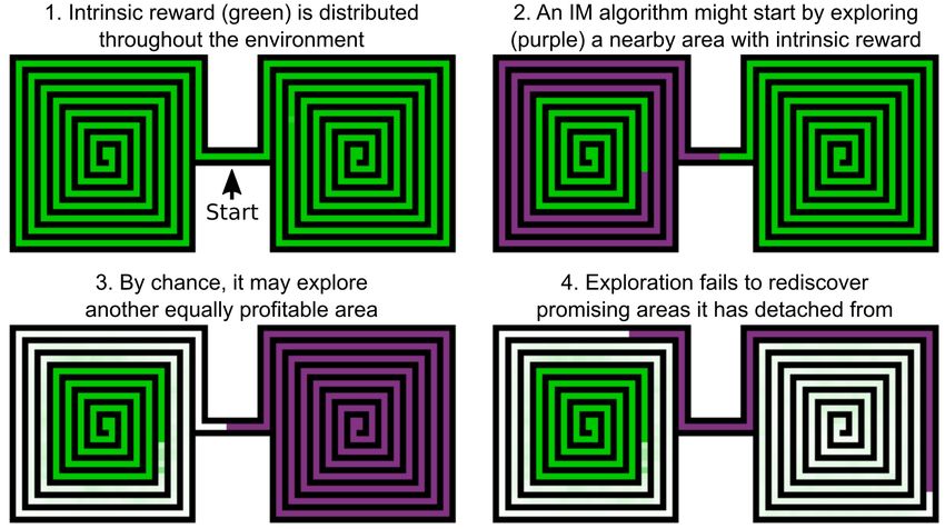
Figure 1: A hypothetical example of detachment in intrinsic motivation (IM) algorithms. Green
areas indicate intrinsic reward, white indicates areas where no intrinsic reward remains, and purple
areas indicate where the algorithm is currently exploring. (1) The agent starts each episode between
the two mazes. (2) It may by chance start exploring the West maze and IM may drive it to learn to
traverse, say, 50% of it. (3) Because current algorithms sprinkle in randomness (either in actions or
parameters) to try to produce new behaviors to find explicit or intrinsic rewards, by chance the agent
may at some point begin exploring the East maze, where it will also encounter a lot of intrinsic reward.
After completely exploring the East maze, it has no explicit memory of the promising exploration
frontier it abandoned in the West maze. It likely would also have no implicit memory of this frontier
due to the problem of catastrophic forgetting [17–20]. (4) Worse, the path leading to the frontier in
the West maze has already been explored, so no (or little) intrinsic motivation remains to rediscover
it. We thus say the algorithm has detached from a frontier of states that provide intrinsic motivation.
As a result, exploration can stall when areas close to where the current agent visits have already
been explored. This problem would be remedied if the agent remembered and returned to previously
discovered promising areas for exploration, which Go-Explore does.

                    Phase 1: explore until solved                                Phase 2: robustify
                                                                                   (if necessary)

  Select state                           Explore            Update            Run imitation learning
                    Go to state
 from archive                          from state           archive             on best trajectory

                  Figure 2: A high-level overview of the Go-Explore algorithm.

high IR, and the former mechanism to return to them. However, the longer, more complex, and more
precise a sequence of actions needs to be in order to reach a previously-discovered high-IR state,
the more likely it is that such stochastic perturbations will “derail” the agent from ever returning to
that state. That is because the needed precise actions are naively perturbed by the basic exploration
mechanism, causing the agent to only rarely succeed in reaching the known state to which it is drawn,
and from which further exploration might be most effective. To address derailment, an insight in
Go-Explore is that effective exploration can be decomposed into first returning to a promising state
(without intentionally adding any exploration) before then exploring further.
Go-Explore is an explicit response to both detachment and derailment that is also designed to achieve
robust solutions in stochastic environments. The version presented here works in two phases (Fig. 2):
(1) first solve the problem in a way that may be brittle, such as solving a deterministic version of the
problem (i.e. discover how to solve the problem at all), and (2) then robustify (i.e. train to be able to

                                                    3
reliably perform the solution in the presence of stochasticity).1 Similar to IM algorithms, Phase 1
focuses on exploring infrequently visited states, which forms the basis for dealing with sparse-reward
and deceptive problems. In contrast to IM algorithms, Phase 1 addresses detachment and derailment
by accumulating an archive of states and ways to reach them through two strategies: (a) add all
interestingly different states visited so far into the archive, and (b) each time a state from the archive
is selected to explore from, first Go back to that state (without adding exploration), and then Explore
further from that state in search of new states (hence the name “Go-Explore”).
An analogy of searching a house can help one contrast IM algorithms and Phase 1 of Go-Explore.
IM algorithms are akin to searching through a house with a flashlight, which casts a narrow beam of
exploration first in one area of the house, then another, and another, and so on, with the light being
drawn towards areas of intrinsic motivation at the edge of its small visible region. It can get lost if at
any point the beam fails to fall on any area with intrinsic motivation remaining. Go-Explore more
resembles turning the lights on in one room of a house, then its adjacent rooms, then their adjacent
rooms, etc., until the entire house is illuminated. Go-Explore thus gradually expands its sphere of
knowledge in all directions simultaneously until a solution is discovered.
If necessary, the second phase of Go-Explore robustifies high-performing trajectories from the archive
such that they are robust to the stochastic dynamics of the true environment. Go-Explore robustifies
via imitation learning (aka learning from demonstrations or LfD [26–29]), a technique that learns how
to solve a task from human demonstrations. The only difference with Go-Explore is that the solution
demonstrations are produced automatically by Phase 1 of Go-Explore instead of being provided
by humans. The input to this phase is one or more high-performing trajectories, and the output is
a robust policy able to consistently achieve similar performance. The combination of both phases
instantiates a powerful algorithm for hard-exploration problems, able to deeply explore sparse- and
deceptive-reward environments and robustify high-performing trajectories into reliable solutions that
perform well in the unmodified, stochastic test environment.
Some of these ideas are similar to ideas proposed in related work. Those connections are discussed in
Section 5. That said, we believe we are the first to combine these ideas in this way and demonstrate
that doing so provides substantial performance improvements on hard-exploration problems.
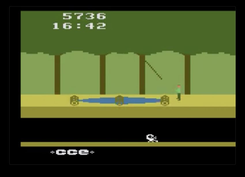
To explore its potential, we test Go-Explore on two hard-exploration benchmarks from the Arcade
Learning Environment (ALE) [30, 31]: Montezuma’s Revenge and Pitfall. Montezuma’s Revenge
has become an important benchmark for exploration algorithms (including intrinsic motivation
algorithms) [4, 16, 32–39] because precise sequences of hundreds of actions must be taken in
between receiving rewards. Pitfall is even harder because its rewards are sparser (only 32 positive
rewards are scattered over 255 rooms) and because many actions yield small negative rewards that
dissuade RL algorithms from exploring the environment.
Classic RL algorithms (i.e. those without intrinsic motivation) such as DQN [3], A3C [40], Ape-
X [41] and IMPALA [42] perform poorly on these domains even with up to 22 billion game frames
of experience, scoring 2,500 or lower on Montezuma’s Revenge and failing to solve level one, and
scoring ≤ 0 on Pitfall. Those results exclude experiments that are evaluated in a deterministic test
environment [43, 44] or were given human demonstrations [26, 27, 45]. On Pitfall, the lack of
positive rewards and frequent negative rewards causes RL algorithms to learn a policy that effectively
does nothing, either standing completely still or moving back and forth near the start of the game
(https://youtu.be/Z0lYamtgdqQ [46]).
These two games are also tremendously difficult for planning algorithms, even when allowed to plan
directly within the game emulator. Classical planning algorithms such as UCT [47–49] (a powerful
form of Monte Carlo tree search [49, 50]) obtain 0 points on Montezuma’s Revenge because the state
space is too large to explore effectively, even with probabilistic methods [30, 51].
Despite being specifically designed to tackle sparse reward problems and being the dominant method
for them, IM algorithms also struggle with Montezuma’s Revenge and Pitfall, although they perform
better than algorithms without IM. On Montezuma’s Revenge, the best such algorithms thus far
average around 11,500 with a maximum of 17,500 [16, 39]. One solved level 1 of the game in 10%
of its runs [16]. Even with IM, no algorithm scores greater than 0 on Pitfall (in a stochastic test
1
Note that this second phase is in principle not necessary if Phase 1 itself produces a policy that can handle
stochastic environments (Section 2.1.3).
4environment, without a human demonstration). We hypothesize that detachment and derailment are
major reasons why IM algorithms do not perform better.
When exploiting easy-to-provide domain knowledge, Go-Explore on Montezuma’s Revenge scores
a mean of 666,474, and its best run scores over 18 million and solves 1,441 levels. On Pitfall,
Go-Explore scores a mean of 59,494 and a maximum of 107,363, which is close to the maximum
of the game of 112,000 points. Without exploiting domain knowledge, Go-Explore still scores a
mean of 43,763 on Montezuma’s Revenge. All scores are dramatic improvements over the previous
state of the art. This and all other claims about solving the game and producing state-of-the-art
scores assume that, while stochasticity is required during testing, deterministic training is allowable
(discussed in Section 2.1.3). We conclude that Go-Explore is a promising new algorithm for solving
hard-exploration RL tasks with sparse and/or deceptive rewards.
2 The Go-Explore Algorithm
The insight that remembering and returning reliably to promising states is fundamental to effective
exploration in sparse-reward problems is at the core of Go-Explore. Because this insight is so flexible
and can be exploited in different ways, Go-Explore effectively encompasses a family of algorithms
built around this key idea. The variant implemented for the experiments in this paper and described
in detail in this section relies on two distinct phases. While it provides a canonical demonstration
of the possibilities opened up by Go-Explore, other variants are also discussed (e.g. in Section 4) to
provide a broader compass for future applications.
2.1 Phase 1: Explore until solved
In the two-phase variant of Go-Explore presented in this paper, the purpose of Phase 1 is to explore
the state space and find one or more high-performing trajectories that can later be turned into a robust
policy in Phase 2. To do so, Phase 1 builds up an archive of interestingly different game states, which
we call “cells” (Section 2.1.1), and trajectories that lead to them. It starts with an archive that only
contains the starting state. From there, it builds the archive by repeating the following procedures:
choose a cell from the current archive (Section 2.1.2), return to that cell without adding any stochastic
exploration (Section 2.1.3), and then explore from that location stochastically (Section 2.1.4). During
this process, any newly encountered cells (as well as how to reach them) or improved trajectories to
existing cells are added to the archive (Section 2.1.5).
2.1.1 Cell representations
One could, in theory, run Go-Explore directly in a high-dimensional state space (wherein each cell
contains exactly one state); however doing so would be intractable in practice. To be tractable in
high-dimensional state spaces like Atari, Phase 1 of Go-Explore needs a lower-dimensional space
within which to search (although the final policy will still play in the same original state space, in this
case pixels). Thus, the cell representation should conflate similar states while not conflating states
that are meaningfully different.
In this way, a good cell representation should reduce the dimensionality of the observations into a
meaningful low-dimensional space. A rich literature investigates how to obtain good representations
from pixels. One option is to take latent codes from the middle of neural networks trained with
traditional RL algorithms maximizing extrinsic and/or intrinsic motivation, optionally adding auxiliary
tasks such as predicting rewards [52]. Additional options include unsupervised techniques such
as networks that autoencode [53] or predict future states, and other auxiliary tasks such as pixel
control [54].
While it will be interesting to test any or all of these techniques with Go-Explore in future work, for
these initial experiments with Go-Explore we test its performance with two different representations:
a simple one that does not harness game-specific domain knowledge, and one that does exploit
easy-to-provide domain knowledge.
Cell representations without domain knowledge
We found that a very simple dimensionality reduction procedure produces surprisingly good results on
Montezuma’s Revenge. The main idea is simply to downsample the current game frame. Specifically,
5Figure 3: Example cell representation without domain knowledge, which is simply to down-
sample each game frame. The full observable state, a color image, is converted to grayscale and
downscaled to an 11 × 8 image with 8 possible pixel intensities.
we (1) convert each game frame image to grayscale (2) downscale it to an 11 × 8 image with area
interpolation (i.e. using the average pixel value in the area of the downsampled pixel), (3) rescale
pixel intensities so that they are integers between 0 and 8, instead of the original 0 to 255 (Fig. 3).
The downscaling dimensions and pixel-intensity range were found by grid search. The aggressive
downscaling used by this representation is reminiscent of the Basic feature set from Bellemare et al.
[30]. This cell representation requires no game-specific knowledge and is fast to compute.
Cell representations with domain knowledge
The ability of an algorithm to integrate easy-to-provide domain knowledge can be an important asset.
In Montezuma’s Revenge, domain knowledge is provided as unique combinations of the x, y position
of the agent (discretized into a grid in which each cell is 16 × 16 pixels), room number, level number,
and in which rooms the currently-held keys were found. In the case of Pitfall, only the x, y position
of the agent and the room number were used. All this information was extracted directly from pixels
with simple hand-coded classifiers to detect objects such as the main character’s location combined
with our knowledge of the map structure in the two games (Appendix A.3). While Go-Explore
provides the opportunity to leverage domain knowledge in the cell representation in Phase 1, the
robustified neural network produced by Phase 2 still plays directly from pixels only.
2.1.2 Selecting cells
In each iteration of Phase 1, a cell is chosen from the archive to explore from. This choice could be
made uniformly at random, but we can improve upon that baseline in many cases by creating (or
learning) a heuristic for preferring some cells over others. In preliminary experiments, we found
that such a heuristic can improve performance over uniform random sampling (data not shown). The
exact heuristic differs depending on the problem being solved, but at a high level, the heuristics in our
work assign a positive weight to each cell that is higher for cells that are deemed more promising. For
example, cells might be preferred because they have not been visited often, have recently contributed
to discovering a new cell, or are expected to be near undiscovered cells. The weights of all cells are
normalized to represent the probability of each cell being chosen next. No cell is ever given a weight
equal to 0, so that all cells in principle remain available for further exploration. The exact heuristics
from our experiments are described in Appendix A.5.
2.1.3 Returning to cells and opportunities to exploit deterministic simulators
One of the main principles of Go-Explore is to return to a promising cell without added exploration
before exploring from that cell. The Go-Explore philosophy is that we should make returning to
that cell as easy as possible given the constraints of the problem. The easiest way to return to a
cell is if the world is deterministic and resettable, such that one can reset the state of the simulator
to a previous visit to that cell. Whether performing such resets is allowable for RL research is an
interesting subject of debate that was motivated by the initial announcement of Go-Explore [55].
The ability to harness determinism and perform such resets forces us to recognize that there are two
different types of problems we wish to solve with RL algorithms: those that require stochasticity at
test time only, and those that require stochasticity during both testing and training.
We start with the former. Because current RL algorithms can take unsafe actions [56, 57] and require
tremendous amounts of experience to learn [41, 42, 58], the majority of applications of RL in the
6foreseeable future will likely require training in a simulator before being transferred to (and optionally
fine-tuned in) the real world. For example, most work with learning algorithms for robotics train in a
simulator before transferring the solution to the real world; that is because learning directly on the
robot is slow, sample-inefficient, can damage the robot, and can be unsafe [59–61]. Fortunately, for
many domains, simulators are available (e.g. robotics simulators, traffic simulators, etc.). An insight
of Go-Explore is that we can take advantage of the fact that such simulators can be made deterministic
to improve performance, especially on hard-exploration problems. For many types of problems, we
want a reliable final solution (e.g. a robot that reliably finds survivors after a natural disaster) and
there is no principled reason to care whether we obtain this solution via initially deterministic training.
If we can solve previously unsolvable problems, including ones that are stochastic at evaluation (test)
time, via making simulators deterministic, we should take advantage of this opportunity.
There are also cases where a simulator is not available and where learning algorithms must confront
stochasticity during training. To create and test algorithms for this second type of problem, we cannot
exploit determinism and resettability. Examples of this class of problems include when we must
learn directly in the real world (and an effective simulator is not available and cannot be learned),
or when studying the learning of biological animals, including ourselves. We believe Go-Explore
can handle such situations by training goal-conditioned policies [62, 63] that reliably return to cells
in the archive during the exploration phase, which is an interesting area for future research. While
computationally much more expensive, this strategy would result in a fully trained policy at the end
of the exploration phase, meaning there would be no need for a robustification phase at the end. We
note that there are some problems where the environment has forms of stochasticity that prevent the
algorithm from reliably returning to a particular cell, regardless of which action the agent takes (e.g.
in poker, there is no sequence of actions that reliably leads you to a state where you have two aces).
We leave a discussion and study of whether Go-Explore helps in that problem setting for future work.
With this distinction in mind, we can now ask whether Montezuma’s Revenge and Pitfall represent the
first type of domain (where all we care about is a solution that is robust to stochasticity at test time) or
the second (situations where the algorithm must handle stochasticity while training). We believe few
people in the community had considered this question before our initial blog post on Go-Explore [55]
and that it created a healthy debate on this subject. Because Atari games are proxies for the problems
we want to solve with RL, and because both types of problems exist, a natural conclusion is that we
should have benchmarks for each. One version of a task can require stochasticity during testing only,
and another can require stochasticity during both training and testing. All results and claims in this
version of this paper are for the version of these domains that does not require stochasticity during
training (i.e. stochasticity is required during evaluation only). Applying Go-Explore when training is
stochastic remains an exciting avenue of research for the near future.
For problems in which all we care about is a reliable policy at test time, a key insight behind
Go-Explore is that we can first solve the problem (Phase 1), and then (if necessary) deal with
making the solution more robust later (Phase 2). In contrast with the usual view of determinism as
a stumbling block to producing agents that are robust and high-performing, it can be made an ally
during exploration and then the solution extended to nondeterminism afterwards via robustification.
An important domain where such insights can help is robotics, where training is often done in
simulation before policies are transferred to the real world [59–61].
For the experiments in this paper, because we harness deterministic training, we could return to a cell
by storing the sequence of actions that lead to it and subsequently replay those actions. However,
simply saving the state of the emulator (in addition to this sequence of steps) and restoring that state
when revisiting a cell gains additional efficiency. Doing so reduced the number of steps that needed
to be simulated by at least one order of magnitude (Appendix A.8).
Due to the fact that the present version of Go-Explore operates in a deterministic setting during
Phase 1, each cell is associated with an open-loop sequence of instructions that lead to it given the
initial state, not a proper policy that maps any state to an action. A true policy is produced during
robustification in Phase 2 (Section 2.2).
2.1.4 Exploration from cells
Once a cell is reached, any exploration method can be applied to find new cells. In this work the agent
explores by taking random actions for k = 100 training frames, with a 95% probability of repeating
the previous action at each training frame (frames at which the agent is allowed to take an action,
7thus not including any frames skipped due to frame skip, see Appendix A.1). Besides reaching the
k = 100 training frame limit for exploration, exploration is also aborted at the episode’s end (defined
in Appendix A.2), and the action that led to the episode ending is ignored because it does not produce
a destination cell.
Interestingly, such exploration does not require a neural network or other controller, and indeed no
neural network was used for the exploration phase (Phase 1) in any of the experiments in this paper
(we do not train a neural network until Phase 2). The fact that entirely random exploration works so
well highlights the surprising power of simply returning to promising cells before exploring further,
though we believe exploring intelligently (e.g. via a trained policy) would likely improve our results
and is an interesting avenue for future work.
2.1.5 Updating the archive
While an agent is exploring from a cell, the archive updates in two conditions. The first condition is
when the agent visits a cell that was not yet in the archive (which can happen multiple times while
exploring from a given cell). In this case, that cell is added to the archive with four associated pieces
of metadata: (1) how the agent got to that cell (here, a full trajectory from the starting state to that
cell), (2) the state of the environment at the time of discovering the cell (if the environment supports
such an operation, which is true for the two Atari-game domains in this paper), (3) the cumulative
score of that trajectory, and (4) the length of that trajectory.
The second condition is when a newly-encountered trajectory is “better” than that belonging to a
cell already in the archive. For the experiments below, we define a new trajectory as better than
an existing trajectory when the new trajectory either has a higher cumulative score or when it is
a shorter trajectory with the same score. In either case, the existing cell in the archive is updated
with the new trajectory, the new trajectory length, the new environment state, and the new score. In
addition, information affecting the likelihood of this cell being chosen (see Appendix A.5) is reset,
including the total number of times the cell has been chosen and the number of times the cell has
been chosen since leading to the discovery of another cell. Resetting these values is beneficial when
cells conflate many different states because a new way of reaching a cell may actually be a more
promising stepping stone to explore from (so we want to encourage its selection). We do not reset the
counter that records the number of times the cell has been visited because that would make recently
discovered cells indistinguishable from recently updated cells, and recently discovered cells (i.e.
those with low visit counts) are more promising to explore because they are likely near the surface of
our expanding sphere of knowledge.
Because cells conflate many states, we cannot assume that a trajectory from start state A through cell
B to cell C will still reach C if we substitute a different, better way to get from A to B; therefore,
the better way of reaching a cell is not integrated into the trajectories of other cells that built upon
the original trajectory. However, performing such substitutions might work with goal-conditioned or
otherwise robust policies, and investigating that possibility is an interesting avenue for future work.
2.1.6 Batch implementation
We implemented Phase 1 in parallel to take advantage of multiple CPUs (our experiments ran on a
single machine with 22 CPU cores): at each step, a batch of b cells is selected (with replacement)
according to the rules described in Section 2.1.2 and Appendix A.5, and exploration from each of
these cells proceeds in parallel for each. Besides using the multiple CPUs to run more instances of
the environment, a high b also saves time by recomputing cell selection probabilities less frequently,
which is important as this computation accounts for a significant portion of run time as the archive
gets large (though this latter factor could be mitigated in other ways in the future). Because the size
of b also has an indirect effect on the exploration behavior of Go-Explore (for instance, the initial
state is guaranteed to be chosen b times at the very first iteration), it is in effect a hyperparameter,
whose values are given in Appendix A.6.
2.2 Phase 2: Robustification
If successful, the result of Phase 1 is one or more high-performing trajectories. However, if Phase 1
of Go-Explore harnessed determinism in a simulator, such trajectories will not be robust to any
stochasticity, which is present at test time. Phase 2 addresses this gap by creating a policy robust to
8noise via imitation learning, also called learning from demonstration (LfD). Importantly, stochasticity
is added during Phase 2 so that the final policy is robust to the stochasticity it will face during
its evaluation in the test environment. Thus the policy being trained has to learn how to mimic
and/or perform as well as the trajectory obtained from the Go-Explore exploration phase while
simultaneously dealing with circumstances that were not present in the original trajectory. Depending
on the stochasticity of the environment, this adjustment can be highly challenging, but nevertheless is
far easier than attempting to solve a sparse-reward problem from scratch.
While most imitation learning algorithms could be used for Phase 2, different types of imitation
learning algorithms can qualitatively affect the resulting policy. LfD algorithms that try to closely
mimic the behavior of the demonstration may struggle to improve upon it. For this reason, we
chose an LfD algorithm that has been shown capable of improving upon its demonstrations: the
Backward Algorithm from Salimans and Chen [28]. It works by starting the agent near the last state
in the trajectory, and then running an ordinary RL algorithm from there (in this case Proximal Policy
Optimization (PPO) [64]). Once the algorithm has learned to obtain the same or a higher reward than
the example trajectory from that starting place near the end of the trajectory, the algorithm backs the
agent’s starting point up to a slightly earlier place along the trajectory, and repeats the process until
eventually the agent has learned to obtain a score greater than or equal to the example trajectory all
the way from the initial state. Note that a similar algorithm was discovered independently at around
the same time by Resnick et al. [65].
While this approach to robustification effectively treats the expert trajectory as a curriculum for the
agent, the policy is only optimized to maximize its own score, and not actually forced to accurately
mimic the trajectory. For this reason, this phase is able to further optimize the expert trajectories, as
well as generalize beyond them, both of which we observed in practice in our experiments (Section 3).
In addition to seeking a higher score than the original trajectory, because it is an RL algorithm with a
discount factor that prizes near-term rewards more than those gathered later, it also has a pressure
to improve the efficiency with which it collects rewards. Thus if the original trajectory contains
unnecessary actions (like visiting a dead end and returning), such behavior could be eliminated during
robustification (a phenomenon we also observed).
2.3 Additional experimental and analysis details
Comparing sample complexity for RL algorithms trained on Atari games can be tricky due to the
common usage of frame skipping [31, 66], wherein a policy only sees and acts every nth (here, 4)
frame, and that action is repeated for intervening frames to save the computation of running the policy.
Specifically, it can be ambiguous whether the frames that are skipped are counted (which we call
“game frames”) or ignored (which we call “training frames”) when discussing sample complexity. In
this work, we always qualify the word “frame” accordingly and all numbers we report are measured
in game frames. Appendix A.1 further details the subtleties of this issue.
Because the Atari games are deterministic by default, some form of stochasticity needs to be
introduced to provide a stochastic test environment, which is desirable to make Atari an informative
test bed for RL algorithms. Following previous work, we introduce stochasticity into the Atari
environment with two previously employed techniques: random no-ops and sticky actions.
Random no-ops means that the agent is forced to take up to 30 no-ops (do nothing commands) at the
start of the game. Because most Atari games run on a timer that affects whether hazards are present
or not, or where different hazards, items, or enemies are located, taking a random number of no-ops
puts the world into a slightly different state each time, meaning that fixed trajectories (such as the
ones found by Go-Explore Phase 1) will no longer work. Random no-ops were first introduced by
Mnih et al. [3], and they were adopted as a primary source of stochasticity in most subsequent papers
working in the Atari domain [3, 26, 27, 34, 38, 41, 42, 45, 67–73].
While random no-ops prevent single, memorized trajectories from solving Atari games, the remainder
of the game remains deterministic, meaning there is still much determinism that can be exploited.
While several other forms of stochasticity have been proposed (e.g. humans restarts [74], random
frame skips [75], etc.), a particularly elegant form is sticky actions [31], where at each game frame
there exists some probability of repeating the previous action instead of performing a newly chosen
action. This way to introduce stochasticity is akin to how humans are not frame perfect, but may hold
a button for slightly longer than they intended, or how they may be slightly late in pressing a button.
9Because Atari games have been designed for human play, the addition of sticky actions generally
does not prevent a game from being solvable, and it adds some stochasticity to every state in the
game, not just the start. Although our initial blog post [55] only included random no-ops, in this
paper our robustification and all post-robustification test results are produced with a combination
of both random no-ops and sticky actions. All algorithms we compare against in Section 3 and in
Appendix A.9 likewise were tested with some form of stochasticity (in the form of no-ops, sticky
actions, human starts, or some combination thereof), though it is worth noting that, unlike Go-Explore,
most also had to handle stochasticity throughout training. Relevant algorithms that were tested in a
deterministic environment are discussed in Section 5.
All hyperparameters were found by performing a separate grid-search for each experiment. The
final, best performing hyperparameters are listed in Appendix A.6, tables 1 and 2. All confidence
intervals given are 95% bootstrapped confidence intervals computed using the pivotal (also known as
empirical) method [76], obtained by resampling 10,000 times. Confidence intervals are reported with
the following notation: stat (CI: lower – upper) where stat is the statistic (a mean unless otherwise
specified). In graphs containing shaded areas, those areas indicate the 95% percentile bootstrapped
confidence interval of the mean, obtained by resampling 1,000 times. Graphs of the exploration phase
(Phase 1) depict data at approximately every 4M game frames and graphs of the robustification phase
(Phase 2) depict data at approximately every 130,000 game frames.
Because the robustification process can diverge even after finding a solution, the neural network
at the end of training does not necessarily perform well, even if a high-performing solution was
found at some point during this process. To retrieve a neural network that performs well regard-
less of when it was found, all robustification runs (Phase 2) produced a checkpoint of the neural
network approximately every 13M game frames. Because the performance values recorded during
robustification are noisy, we cannot select the best performing checkpoint from those performance
values alone. As such, at the end of each robustification run, out of the checkpoints with the lowest
max_starting_point (or close to it), a random subset of checkpoints (between 10 and 50) was
tested to evaluate the performance of the neural network stored within that checkpoint. We test a
random subset because robustification runs usually produce more successful checkpoints then we can
realistically test. The highest-scoring checkpoint for each run was then re-tested to account for the
selection bias inherent in selecting the best checkpoint. The scores from this final retest are the ones
we report.
The neural network from each checkpoint is evaluated with random no-ops and sticky actions until at
least 5 scores for each of the 31 possible starting no-ops (from 0 to 30 inclusive) are obtained. The
mean score for each no-op is then calculated and the final score for the checkpoint is the grand mean
of the individual no-op scores. Unless otherwise specified, the default time limit of 400,000 game
frames imposed by OpenAI Gym [75] is enforced.
3 Results
3.1 Montezuma’s Revenge
3.1.1 Without domain knowledge in the cell representation
In this first experiment, we run Go-Explore on Montezuma’s Revenge with the downsampled image
cell representation, which does not require game-specific domain knowledge. Despite the simplicity
of this cell representation, Phase 1 of Go-Explore solves level 1 in 57% of runs after 1.2B game
frames (a modest number by modern standards [41, 42]), with one of the 100 runs also solving level
2, and visits a mean of 35 rooms (CI: 33 – 37) (Fig. 4a). The number of new cells being discovered is
still increasing linearly after 1.2B game frames, indicating that results would likely be even better
were it run longer (Fig. 4b). Phase 1 of Go-Explore achieves a mean score of 57,439 (CI: 47,843 –
67,224) (Fig. 4c). Level 1 was solved after a mean of 640M (CI: 567M – 711M) game frames, which
took a mean of 10.8 (CI: 9.5 – 12.0) hours on a single, 22-CPU machine (note that these level 1
numbers exclude the runs that never solved level 1 after 1.2B game frames). See Appendix A.8 for
more details on performance.
Amusingly, Go-Explore discovered a little-known bug in Montezuma’s Revenge called the “treasure
room curse” [77]. If the agent performs a specific sequence of actions, it can remain in the treasure
room (the final room before being sent to the next level) indefinitely, instead of being automatically
1015,000 60,000
30
Found Rooms
Found Cells
Best Score
10,000 40,000
20 State of the art
Human Expert
10 5,000 20,000
0 0 0 Average Human
0.0 0.5 1.0 0.0 0.5 1.0 0.0 0.5 1.0
Game Frames 1e9 Game Frames 1e9 Game Frames 1e9
(a) Number of rooms found (b) Number of cells found (c) Maximum score in archive
Figure 4: Performance of the exploration phase of Go-Explore with downscaled frames on
Montezuma’s Revenge. Lines indicating human and the algorithmic state of the art are for compar-
ison, but recall that the Go-Explore scores in this plot are on a deterministic version of the game
(unlike the post-Phase 2 scores presented in this section).
Demo 0
5,000 30,000 Demo 1
Demo 2
25,000 Demo 3
4,000
Max Starting Point
Max Starting Point Demo 4
20,000 Demo 5
3,000 Demo 6
15,000 Demo 7
Demo 8
2,000 Demo 9
10,000
1,000 5,000
0 0
0.0 0.2 0.4 0.6 0.8 1.0 1.2 1.4 1.6 0.0 0.2 0.4 0.6 0.8 1.0 1.2 1.4 1.6
Game Frames 1e9 Game Frames 1e9
(a) Failed robustification with 1 demonstration (b) Successful robustification with 10 demonstrations
Figure 5: Examples of maximum starting point over training for robustifying using different
numbers of demonstrations. Success is achieved as soon as any of the curves gets sufficiently close
(e.g. within 50 units) to 0, because that means the agent is able to perform as well as at least one of
the demonstrations.
moved to the next level after some time. Because gems giving 1,000 points keep appearing in the
treasure room, it is possible to easily achieve very high scores once it has been triggered. Finding bugs
in games and simulators, as Go-Explore did, is an interesting reminder of the power and creativity of
optimization algorithms [6], and is commercially valuable as a debugging tool to identify and fix such
bugs before shipping simulators and video games. A video of the treasure room curse as triggered by
Go-Explore is available at https://youtu.be/civ6OOLoR-I.
In 51 out of the 57 runs that solved level 1, the highest-scoring trajectory found by Go-Explore
exploited the bug. To prevent scores from being inflated due to this bug, we filtered out trajectories
that triggered the treasure room curse bug when extracting the highest scoring trajectory from each
run of Go-Explore for robustification (Appendix A.4 provides details).
As mentioned in Section 2.2, we used Salimans & Chen’s Backward Algorithm [28] for robustification.
However, we found it somewhat unreliable in learning from a single demonstration (Fig. 5a). Indeed,
only 40% of our attempts at robustifying trajectories that solved level 1 were successful when using a
single demonstration.
However, because Go-Explore can produce many demonstrations, we modified the Backward Algo-
rithm to simultaneously learn from multiple demonstrations (details in Appendix A.7). To simulate
the use case in which Phase 1 is run repeatedly until enough successful demonstrations (in this case
10) are found, we extracted the highest scoring non-bug demonstration from each of the 57 out of
11Go-Explore
40,000
Human Expert
30,000
Score
20,000
PPO+CoEX
10,000 DQN-PixelCNN RND
Reactor
Feature-EB
Avg. Human DQN-CTS UBE
DDQN A3C-CTS IMPALA
SARSA Gorila A3C Ape-X
0 Linear DQN MP-EB Pop-Art ES C51 Rainbow
Prior. DQN
Duel. DQN BASS-hash
2013 2014 2015 2016 2017 2018 2019
Time of publication
Figure 6: History of progress on Montezuma’s Revenge vs. the version of Go-Explore that does
not harness domain knowledge. Go-Explore significantly improves on the prior state of the art.
These data are presented in tabular form in Appendix A.9.
100 Phase 1 runs that had solved level 1, and randomly assigned them to one of 5 non-overlapping
groups of 10 demonstrations (7 demonstrations were left over and ignored), each of which was used
for a robustification run. When training with 10 demonstration trajectories, all 5 robustification runs
were successful. Fig. 5b shows an example of successful robustification with 10 trajectories.
In the end, our robustified policies achieve a mean score of 43,763 (CI: 36,718 – 50,196), substantially
higher than the human expert mean of 34,900 [27]. All policies successfully solve level 1 (with a
99.8% success rate over different stochastic evaluations of the policies), and one of our 5 policies
also solves level 2 100% of the time. Fig. 6 shows how these results compare with prior work.
Surprisingly, the computational cost of Phase 2 is greater than that of Phase 1. These Phase 2 results
were achieved after a mean of 4.35B (CI: 4.27B – 4.45B) game frames of training, which took a
mean of 2.4 (CI: 2.4 – 2.5) days of training (details in Appendix A.8).
3.1.2 With domain knowledge in the cell representation
On Montezuma’s Revenge, when harnessing domain knowledge in its cell representation (Sec-
tion 2.1.1), Phase 1 of Go-Explore finds a total of 238 (CI: 231 – 245) rooms, solves a mean of 9.1
(CI: 8.8 – 9.4) levels (with every run solving at least 7 levels), and does so in roughly half as many
game frames as with the downscaled image cell representation (Fig. 7a). Its scores are also extremely
high, with a mean of 148,220 (CI: 144,580 – 151,730) (Fig. 7c). These results are averaged over 50
runs.
As with the downscaled version, Phase 1 of Go-Explore with domain knowledge was still discovering
additional rooms, cells, and ever-higher scores linearly when it was stopped (Fig. 7). Indeed, because
every level of Montezuma’s Revenge past level 3 is nearly identical to level 3 (except for the scores
on the screen and the stochastic timing of events) and because each run had already passed level 3, it
would likely continue to find new rooms, cells, and higher scores forever.
Domain knowledge runs spend less time exploiting the treasure room bug because we preferentially
select cells in the highest level reached so far (Appendix A.5). Doing so encourages exploring new
levels instead of exploring the treasure rooms on previous levels to keep exploiting the treasure room
bug. The highest final scores thus come from trajectories that solved many levels. Because knowing
the level number constitutes domain knowledge, non-domain knowledge runs cannot take advantage
of this information and are thus affected by the bug more.
12250 50,000 150,000
Found Domain Knowledge Cells
200 40,000 125,000
Go-Explore
Found Rooms 150 100,000
Best Score
(no domain 30,000
knowledge)
Go-Explore 75,000
100 (domain 20,000
knowledge) 50,000
50 10,000 25,000 Human Expert
0 State of the art 0 0 Average Human
0.0 0.5 1.0 0.0 0.5 1.0 0.0 0.5 1.0
Game Frames 1e9 Game Frames 1e9 Game Frames 1e9
(a) Number of rooms found (b) Number of cells found (c) Maximum score in archive
Figure 7: Performance on Montezuma’s Revenge of Phase 1 of Go-Explore with and without
domain knowledge. The algorithm finds more rooms, cells, and higher scores with the easily
provided domain knowledge, and does so with a better sample complexity. For (b), we plot the
number of cells found in the no-domain-knowledge runs according to the more intelligent cell
representation from the domain-knowledge run to allow for an equal comparison.
In terms of computational performance, Phase 1 with domain knowledge solves the first level after
a mean of only 57.6M (CI: 52.7M – 62.3M) game frames, corresponding to 0.9 (CI: 0.8 – 1.0)
hours on a single 22-CPU machine. Solving level 3, which effectively means solving the entire
game as discussed above, is accomplished in a mean of 173M (CI: 164M – 182M) game frames,
corresponding to 6.8 (CI: 6.2 – 7.3) hours. Appendix A.8 provides full performance details.
For robustification, we chose trajectories that solve level 3, truncated to the exact point at which level
3 is solved because, as mentioned earlier, all levels beyond level 3 are nearly identical aside from the
pixels that display the score, which of course keep changing, and some global counters that change
the timing of aspects of the game like when laser beams turn on and off.
We performed 5 robustification runs with demonstrations from the Phase 1 experiments above, each
of which had a demonstration from each of 10 different Phase 1 runs. All 5 runs succeeded. The
resulting mean score is 666,474 (CI: 461,016 – 915,557), far above both the prior state of the art and
the non-domain knowledge version of Go-Explore. As with the downscaled frame version, Phase 2
was slower than Phase 1, taking a mean of 4.59B (CI: 3.09B – 5.91B) game frames, corresponding to
a mean of 2.6 (CI: 1.8 – 3.3) days of training.
The networks show substantial evidence of generalization to the minor changes in the game beyond
level 3: although the trajectories they were trained on only solve level 3, these networks solved a
mean of 49.7 levels (CI: 32.6 – 68.8). In many cases, the agents did not die, but were stopped by
the maximum limit of 400,000 game frames imposed by default in OpenAI Gym [75]. Removing
this limit altogether, our best single run from a robustified agent achieved a score of 18,003,200 and
solved 1,441 levels during 6,198,985 game frames, corresponding to 28.7 hours of game play (at
60 game frames per second, Atari’s original speed) before losing all its lives. This score is over an
order of magnitude higher than the human world record of 1,219,200 [78], thus achieving the strictest
definition of “superhuman” performance. A video of the agent solving the first ten levels can be seen
here: https://youtu.be/gnGyUPd_4Eo.
Fig. 8 compares the performance of Go-Explore to historical results (including the previous state of
the art), the no-domain-knowledge version of Go-Explore, and previous imitation learning work that
relied on human demonstrations to solve the game. The version of Go-Explore that harnesses domain
knowledge dramatically outperforms them all. Specifically, Go-Explore produces scores over 9 times
greater than those reported for imitation learning from human demonstrations [28] and over 55 times
the score reported for the prior state of the art without human demonstrations [39].
That Go-Explore outperforms imitation learning plus human demonstrations is particularly notewor-
thy, as human-provided solutions are arguably a much stronger form of domain knowledge than that
provided to Go-Explore. We believe that this result is due to the higher quality of demonstrations
that Go-Explore was able to produce for Montezuma’s Revenge vs. those provided by humans in the
previous imitation learning work. The demonstrations used in our work range in score from 35,200
to 51,900 (lower than the final mean score of 148,220 for Phase 1 because these demonstrations are
13No Domain Knowledge Go-Explore (domain knowledge)
Human Demonstration
Domain Knowledge
600,000
500,000
Score 400,000
300,000
200,000
Ape-X DQfD TDC+CMC
100,000 LfSD (best)
DQN-CTS Go-Explore
Human Expert DQN-PixelCNN
SARSA Gorila DDQN A3C DQfD RND
0 Linear DQN MP-EB A3C-CTS Ape-X PPO+CoEX
Duel. DQN BASS-hash UBE DeepCS
2013 2014 2015 2016 2017 2018 2019
Time of publication
Figure 8: Historical progress on Montezuma’s Revenge vs. the version of Go-Explore that
harnesses domain knowledge. With domain knowledge, Go-Explore dramatically outperforms
prior work, the no-domain-knowledge version of Go-Explore, and even prior work with imitation
learning that was provided the solution in the form of human demonstrations. The data are presented
in tabular form in Appendix A.9.
limited to only solving up to level 3) and most importantly, they all solve level 3. The demonstration
originally used with the Backward Algorithm [28] reaches a score of 71,500 but doesn’t solve level 3,
thus preventing it from generalizing to further levels. The demonstrations used in DQfD and Ape-X
DQfD [26, 27] only range in score from 32,300 to 34,900. In this last case, it is not clear whether
level 3 was solved in any of the demonstrations, but we believe this is unlikely given the reported
scores because they are lower than the lowest level-3-solving scores found by Go-Explore and given
the fact that the human demonstration used by the Backward Algorithm scored twice as high without
solving level 3.
One interesting benefit of a robustification phase with an imitation learning algorithm that does not
try to mimic the original demonstration is that it can improve upon that demonstration. Because of
the discount on future rewards that exists in the base RL algorithm PPO, there is a pressure to remove
inefficiencies in the demonstration. Videos of Go-Explore policies reveal efficient movements. In
contrast, IM algorithms specifically reward reaching novel states, meaning that policies produced by
them often do seemingly inefficient things like deviating to explore dead ends or jumping often to
touch states only accessible by jumping, even though doing so is not necessary to gain real reward.
An example of a Deep Curiosity Search agent [37] performing such inefficient jumps can be viewed at
https://youtu.be/-Fy2va3IbQU, and a random network distillation [16] IM agent can be viewed
at https://youtu.be/40VZeFppDEM. These results suggest that IM algorithms could also benefit
from a robustification phase in which they focus only on real-game reward once the IM phase has
sufficiently explored the state space.
3.2 Pitfall
We next test Go-Explore on the harder, more deceptive game of Pitfall, for which all previous RL
algorithms scored ≤ 0 points, except those that were evaluated on the fully deterministic version of
the game [43, 44] or relied on human demonstrations [26, 27, 45]. As with Montezuma’s Revenge,
we first run Go-Explore with the simple, domain-general, downscaled representation described in
Section 2.1.1, with the same hyperparameters. With these settings, Go-Explore is able to find 22
rooms, but it is unable to find any rewards (Fig. 9). We believe that this number of rooms visited is
greater than the previous state of the art, but the number of rooms visited is infrequently reported
so we are unsure. In preliminary experiments, Go-Explore with a more fine-grained downscaling
14You can also read