GPSView: A Scenic Driving Route Planner
←
→
Page content transcription
If your browser does not render page correctly, please read the page content below
GPSView: A Scenic Driving Route Planner
YAN-TAO ZHENG, Institute for Infocomm Research
SHUICHENG YAN, ZHENG-JUN ZHA, National University of Singapore
YIQUN LI, Institute for Infocomm Research                                                                                                                       3
XIANGDONG ZHOU, Fudan University
TAT-SENG CHUA, National University of Singapore
RAMESH JAIN, University of California, Irvine

GPS devices have been widely used in automobiles to compute navigation routes to destinations. The generated driving route
targets the minimal traveling distance, but neglects the sightseeing experience of the route. In this study, we propose an aug-
mented GPS navigation system, GPSView, to incorporate a scenic factor into the routing. The goal of GPSView is to plan a
driving route with scenery and sightseeing qualities, and therefore allow travelers to enjoy sightseeing on the drive. To do so,
we first build a database of scenic roadways with vistas of landscapes and sights along the roadside. Specifically, we adapt
an attention-based approach to exploit community-contributed GPS-tagged photos on the Internet to discover scenic roadways.
The premise is: a multitude of photos taken along a roadway imply that this roadway is probably appealing and catches the
public’s attention. By analyzing the geospatial distribution of photos, the proposed approach discovers the roadside sight spots,
or Points-Of-Interest (POIs), which have good scenic qualities and visibility to travelers on the roadway. Finally, we formulate
scenic driving route planning as an optimization task towards the best trade-off between sightseeing experience and traveling
distance. Testing in the northern California area shows that the proposed system can deliver promising results.
Categories and Subject Descriptors: H.1.m [Models and Principles]: Miscellaneous
General Terms: Algorithm, Experimentation
Additional Key Words and Phrases: Scenic driving, route planning, geo-mining
ACM Reference Format:
Zheng, Y.-T., Yan, S., Zha, Z.-J., Li, Y., Zhou, X., Chua, T.-S., and Jain, R. 2013. GPSView: A scenic driving route planner. ACM
Trans. Multimedia Comput. Commun. Appl. 9, 1, Article 3 (February 2013), 18 pages.
DOI = 10.1145/2422956.2422959 http://doi.acm.org/10.1145/2422956.2422959

1. INTRODUCTION
In the last decade, Global Positioning System (GPS) technologies have been widely used to provide
navigation and direction services, especially in automobiles. By visualizing the driving route in a map
image, an in-car GPS navigator has made the navigation in driving much easier. Though GPS devices

Authors’ addresses: Y.-T. Zheng (corresponding author), Institute for Infocomm Research, Fusionopolis Way, Singapore 138632;
email: yantaozheng@gmail.com; S. Yan, Z.-J. Zha, National University of Singapore, Singapore; Y. Li, Institute for Infocomm
Research, Fusionopolis Way, Singapore 138632; X. Zhou, Fudan University, T.-S. Chua, National University of Singapore,
Singapore; R. Jain, University of California, Irvine, CA.
Permission to make digital or hard copies of part or all of this work for personal or classroom use is granted without fee provided
that copies are not made or distributed for profit or commercial advantage and that copies show this notice on the first page
or initial screen of a display along with the full citation. Copyrights for components of this work owned by others than ACM
must be honored. Abstracting with credit is permitted. To copy otherwise, to republish, to post on servers, to redistribute to
lists, or to use any component of this work in other works requires prior specific permission and/or a fee. Permissions may be
requested from Publications Dept., ACM, Inc., 2 Penn Plaza, Suite 701, New York, NY 10121-0701 USA, fax +1 (212) 869-0481,
or permissions@acm.org.
c 2013 ACM 1551-6857/2013/02-ART3 $15.00
DOI 10.1145/2422956.2422959 http://doi.acm.org/10.1145/2422956.2422959

                        ACM Transactions on Multimedia Computing, Communications and Applications, Vol. 9, No. 1, Article 3, Publication date: February 2013.
3:2     •      Y.-T. Zheng et al.

Fig. 1. Route (b) is the shortest traveling path recommended by GPS system, while route (a) is a scenic detour with ocean view.
For better viewing, please see the original color pdf file.

have made the navigation of a driving journey easy and convenient, the traveling part could still be
boring, if not exhausting. To date, most GPS navigation devices only consider the traveling distance
and time when designing a driving route, but neglect the visual and scenic attributes of the route. In
this study, we propose an augmented GPS navigation system, GPSView, to incorporate a scenic factor
into the routing. The goal of GPSView is to plan a driving route with the scenic beauties of landscape
and sights, and therefore allow travelers to enjoy sightseeing on the drive. For example in Figure 1,
route (b) going through a neighborhood has the minimal traveling distance between the starting and
ending point, while route (a) might be a better alternative, as travelers can enjoy the ocean view
whilst driving along. Effectively, GPSView intends to convert people’s driving to their destinations into
sightseeing road trips, by suggesting a detour route with scenic landscapes and reasonable traveling
distance.
   An intuitive solution to GPSView is to design a traveling route that passes by a few tourist attrac-
tions or landmarks. This solution looks plausible but not valid due to two reasons. First, scenic driving
is a sightseeing activity that takes place in automobiles when people are traveling. This traveling
nature makes it different from other sightseeing activities like visiting a landmark. Second, scenic
driving is a continuous traveling experience, while tourist attractions, such as buildings, monuments,
etc., are usually discrete geographical “points” with small geospatial scope, which are not sufficient to
enhance the interestingness of the whole route. Besides, tourist attractions may not be visible from
the road.
   To plan the scenic route, we resort to another geographical concept, a scenic roadway. A scenic road-
way is defined as a thoroughfare that passes through landscapes and sights and affords vistas along
its roadsides. The “17 Mile Drive” at Monterey, California and “The Embarcadero” at San Francisco in
Figure 1 are examples of scenic streets/roads, as they offer ocean views and cityscapes of San Fran-
cisco. Some states in the United States like California also have designated scenic roads, such as the
California State Scenic Highway System. In contrast to tourist attractions, the scenic roadway differs
ACM Transactions on Multimedia Computing, Communications and Applications, Vol. 9, No. 1, Article 3, Publication date: February 2013.

GPSView: A Scenic Driving Route Planner                 •     3:3

Fig. 2. “Cannery Row, Monterey” in (a) and “The Embarcadero, San Francisco” in (b) are two examples of scenic streets/roads.
The Embarcadero resides in the famous touristic area in San Francisco, while Cannery Row l locates in the residential suburb
in Monterey. For better viewing, please see the original color pdf file.

in several aspects. First, as a traveling path, the scenic roadway has a elongated geographical scope,
while landmarks are usually well-known sites or buildings of a small geographical scope. By its nature,
the scenic roadway is particularly suited for tourist traveling by automobile, while the landmark better
fits tourists who intend to have in-depth sightseeing on foot. Second, the scenic spots along a roadway
are not necessarily famous sights like tourist attractions and landmarks. It is the overall immersive
scenic environment along the roadside that makes it a pleasant driving experience.
   Planning a traveling route based on scenic roadways, however, has several major challenges: (1) there
is no readily available database of scenic roadways; (2) the scenic and aesthetic qualities of a roadway
are difficult to estimate, as they depend on the sightseeing experience of the travel in the roadway;
(3) besides aesthetic qualities, scenic spots on the roadside must be visible from the roadways to provide
sightseeing experience to travelers; and (4) an efficient and effective algorithm is needed to compute
the route that optimizes both sightseeing experience and traveling distance in real time.
   We tackle the aforementioned issues as follows. To estimate the scenic quality of a roadway, we ex-
ploit the geographically calibrated photos available at photo-sharing Web sites, like flickr.com. These
GPS-tagged photos provide a bridge connecting geography, time, and visual information together
[Jesdanun 2008]. Inferring scenic quality from visual contents of photos is an intuitive solution to dis-
cover scenic roadways. The complexity of visual learning is, however, prohibiting. Instead, we adapt an
attention-based1 approach to exploit the GPS-tagged photos to estimate the interestingness or scenic
qualities of a roadway. The premise is: a photo, especially a tourist photo, usually reflects the photog-
rapher’s attention on its tagged geolocation. A multitude of photos distributed along a thoroughfare
implies that this thoroughfare is probably interesting and catches the public’s attention. Discover-
ing scenic roadways is then cast as a task of analyzing the geospatial distribution of photos. To en-
sure good visibility of a roadside scenic spot, we analyze the dominant geospatial orientation of its

1 The attention-based method here refers to the aspect that snapping a photo of an object/scene reflects some attention of the

tourist on it implicitly. It is different from the “attention model” in image analysis.
     ACM Transactions on Multimedia Computing, Communications and Applications, Vol. 9, No. 1, Article 3, Publication date: February 2013.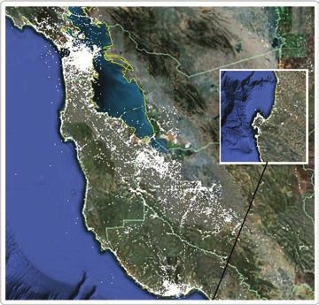
3:4     •      Y.-T. Zheng et al.

photos. The rational is: if a scenic spot is visible from a roadway, then its photos are highly probable to
be distributed along the roadway. Finally, based on the discovered scenic roadways, we formulate the
scenic driving route planning as an optimization task that seeks the best trade-off between sightseeing
experience and traveling distance, in the framework of the Bellman-Ford algorithm [Bellman 1958].
  Overall, this study aims to discover scenic roadways and plan pleasant driving routes for travelers
to have sightseeing on the drive. To the best of our knowledge, this is the first attempt to substantiate
the discovery of a scenic roadways and the optimal routing for both traveling and sightseeing on the
drive. The main contributions are as follows.
—We propose an attention-based approach to discover scenic roadways from a collection of GPS-tagged
 photos. The proposed approach ensures that the roadside sight spots have both good scenic qualities
 and visibility, so that travelers may have an immersive sightseeing experience on the drive.
—We develop a real-time route planning process that optimizes both driving distance and the sight-
 seeing experience.
We evaluate the proposed system on a number of localities in northern California ranging from touris-
tic areas to residential suburbs. Experiments show that the proposed system can deliver promising
results.
   The rest of the article is organized as follows. We first review related literature work in Section
2 and then introduce the system overview in Section 3. Section 4 elaborates on the implementation
details of the proposed GPSView system and Section 5 presents the experiments. Finally, we present
the conclusive remarks along with discussion for future work in Section 6.

2.    RELATED WORK
In recent years, the advent of media-sharing services, such as FlickrTM , has led to voluminous
community-contributed photos available on the Internet [Torniai et al. 2007; Chippendale et al. 2009;
Crandall et al. 2009; Kalogerakis et al. 2009]. Together with socially generated textual and spatiotem-
poral metadata, these enriched multimedia data have spurred much research on discovering knowl-
edge and patterns of our human society [Jing et al. 2006; Zheng et al. 2009a]. Kennedy et al. [2007]
proposed to discover aggregate knowledge of a geographical area, by analyzing spatiotemporal pat-
terns of tags of Flickr photos in the area. Similarly, Rattenbury et al. [2007] and Yanai et al. [2009]
analyzed the spatiotemporal distribution of photo tags to reveal the inter-relation between word con-
cepts (namely photo tags), geographical locations and events. Snavely et al. [2006; 2008] and Goesele
et al. [2007] attempted to build virtual tourism of landmarks by constructing 3D visualization models
from landmark photos. Similarly, Agarwal et al. [2009] reconstructed 3D scenes of tourist sights from
photos on the Internet. Li et al. [2008] and Zheng et al. [2009a] learned the geographical locations
and visual models of landmarks from community contributed photos on the Internet. Kennedy et al.
[2007] and Hao et al. [2009; 2010] attempted to build the visual and textual summarization of land-
marks from the community contributed geo-tagged photos and online travelogues respectively. The
commonality between the aforementioned work and this study is that all of them aim to extract some
knowledge and patterns from photos with textual and spatiotemporal metadata. The difference is that
our approach focuses on discovering scenic roadways with scenic and visual attributes. In contrast to a
tourist landmark, a scenic roadway is a traveling path with vistas of landscapes and sights, and thus
particularly suited for sightseeing on the drive. The scenic sight of a roadway is not necessarily as well
known as a tourist landmark. A roadside place can be part of a scenic roadway, as long as it offers a
scenic landscape and visual interestingness.
  The proposed GPSView system is also closely related to tour route recommendation systems [Lewa
and McKerchera 2006; Asakura and Iryo 2007; De Choudhury et al. 2010]. Choudhury et al. proposed
ACM Transactions on Multimedia Computing, Communications and Applications, Vol. 9, No. 1, Article 3, Publication date: February 2013.
GPSView: A Scenic Driving Route Planner                 •     3:5

Fig. 3. System framework of GPSView. GPSView consists of two major modules: (1) scenic roadway discovery and (2) scenic
driving route planning. The scenic roadway discovery module mines a set of scenic thoroughfares with attractive sights based
on GPS-tagged photos, and the scenic driving route planning module then computes the driving route that optimizes both
sightseeing experience and traveling distance.

a system to construct intra-city travel itineraries for vacation planning. Elias and Sester [2006] at-
tempted to recommend a navigation route that traverses along a set of tourist landmarks with minimal
complexity of route description, while Zhang et al. [2008] focused on searching tourist routes to visit a
few tourist attractions with the shortest traveling distance. Similarly, Kawai et al. [2009] developed a
personalized tour recommendation system to visit tourist sights around a tour destination. The target
of the preceding approaches is to visit a set of destinations with a minimal traveling distance. In con-
trast, the focus of this study is not only on the traveling distance, but also the “traveling” experience.
Namely, it aims to plan scenic driving routes for travelers to experience sightseeing on the drive.
   The proposed GPSView can be regarded as an augmented version of existing commercial geographi-
cal information services, such as Google Maps,2 Yahoo! Local Maps,3 and Geobase,4 etc. The argumen-
tation in GPSView is to incorporate a scenic factor into route planning. Meanwhile, GPSView leverages
the functionalities of these services to compute the driving route and direction with minimal traveling
distance/time.
   Some earlier studies have explored dynamic route selection in route planning [Hochmair 2007;
Hochmair and Navratil 2008]. Hochmair [2007] and Winter [2002] emphasized the cost of turning
in designing an optimized journey in a traffic network, while Hochmair [2007] focuses on a set of op-
timized routes that allow the user to dynamically select the preferred route. With respect to scenery
and sightseeing, the work in Hochmair and Navratil [2008] is closest to this article. The system in
Hochmair and Navratil [2008] searched for scenic routes in a street network. The main idea is to re-
duce the traveling cost of choosing a street segment that runs within a certain buffer distance of attrac-
tive locations. In contrast, the proposed method focuses on discovering scenic roadways, which provide
a scenic and aesthetic roadside driving environment. Some Web services, such as www.byways.org,
also provide route planning for scenic driving. The major difference of our system is that we aim to
automatically build a database of scenic roadways by utilizing geo-tagged photos on the Internet.

3.   SYSTEM OVERVIEW
Figure 3 illustrates the system framework of the GPSView, which consists of two major modules, that
is, scenic roadway discovery and the scenic driving route planning. In the module of scenic roadway
discovery, we discover a set of thoroughfares with scenic and visual attributes from GPS-tagged photos

2 http://maps.google.com.
3 http://map.yahoo.com.
4 http://www.geobase.info.

      ACM Transactions on Multimedia Computing, Communications and Applications, Vol. 9, No. 1, Article 3, Publication date: February 2013.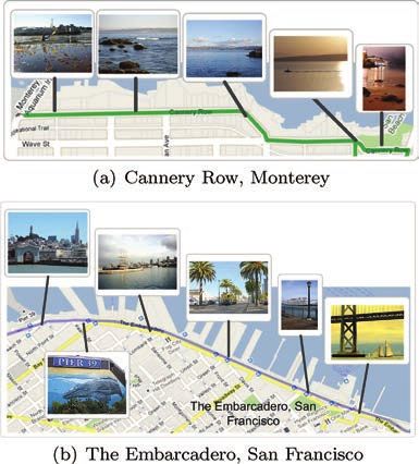
3:6     •      Y.-T. Zheng et al.

within a given local region. The advantage of utilizing photos on the Internet is that the voluminous
photos allow GPSView to easily scale up to many regions and cities by downloading photos tagged
there. To discover scenic roadways, two issues are tackled, which are (1) the roadside sight spots must
have visual or scenic qualities; and (2) the discovered roadside scenic spot or Point-Of-Interest (POI)
must be visible from the roadway. To resolve the first issue, we rely on analyzing the distributions
of tourist photos, as a major interest of tourists is sightseeing and a concentration of tourist photos
may indicate a location that is probably an interesting and scenic sight. To tackle the second issue,
we exploit the dominant geospatial orientation of the photos of a roadside scenic POI to determine its
visibility from the road. The rational is: if a POI is visible from a roadway, then its photos are highly
probable to be distributed along the roadway. Based on the discovered scenic roadways, the module of
scenic route planning takes a starting point and a destination as input and computes the driving route
that optimizes both sightseeing experience and traveling distance.

4.    APPROACH
In this section, we elaborate on the implementation details of the GPSView. We will show how scenic
roadways are mined from community-contributed GPS-tagged photos and how a scenic driving route
is computed by optimizing both sightseeing experience and traveling distance.

4.1 Learning Scenic Roadways
Given a set of GPS-tagged photos P = { p} with GPS coordinates {℘ p}, photo taken time {tp} and up-
loader id {θ p}, our task is to discover scenic roadways with landscapes and sights within a local region.
Here we define a scenic roadway as follows.

  Definition 1. A scenic roadway is a thoroughfare that passes by a series of landscapes and sights
and affords vistas of notable aesthetic, geological, historical, cultural, and touristic qualities along its
roadside.

  The premise of our approach is: if a large number of photos are densely distributed along a roadway,
then this roadway is a scenic one with a series of scenic sight spots, or Points-Of-Interest (POIs), on the
roadside. Clustering on photos is an intuitive solution. One issue, however, needs to be tackled first.
The GPS-tagged photos used in the scenic roadway mining must be able to correctly reflect the popular
appeal of a geolocation. In other words, these photos should be about its tagged geolocation, but not
some unrelated events, like a party or event held near a roadway. To tackle this issue, we utilize only
tourist photos in the mining process. The rational is that as a major interest of tourists is sightseeing,
photos taken by tourists tend to be about interesting and scenic sights.
   4.1.1 Selecting Tourist Photos. The selection of tourist photos relies on the analysis of the spa-
tiotemporal distribution of photos. Due to the mobile nature of tourist sightseeing, photos taken by
a tourist tend to be spread over a large spatial extent within a tour destination. This spatiotempo-
ral pattern of tourist photos provides the basis for discriminating tourist versus non-tourist photos.
Specifically, we first construct the spatiotemporal movement sequence of a photographer by concate-
nating photos in the order of their time-stamp on a daily basis. We then classify these spatiotemporal
photo trajectories to tourist and non-tourist trajectories, based on the tourist mobility characteristics.
The premise is the mobile nature of tourist sightseeing. In a probabilistic perspective, this mobility
complexity leads to a geospatial distribution of photos with reasonably high entropy.
   Mobility entropy of photos. We therefore exploit this mobility entropy to discriminate the tourist and
non-tourist movement trajectories, by utilizing the concept of Shannon entropy in information theory.
ACM Transactions on Multimedia Computing, Communications and Applications, Vol. 9, No. 1, Article 3, Publication date: February 2013.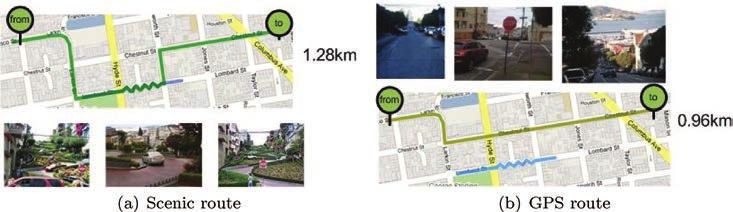
GPSView: A Scenic Driving Route Planner                 •     3:7

Let p(x, y) denote the geospatial density of photos with geospatial coordinates (x, y)5 pertaining to a
photographer/uploader. The mobility entropy Hmob(S) of a movement trajectory S =  is computed as follows. We have

                                                                     n
                                                                       m
                                                    Hmob(S) = −                 pi j log pi j ,                                           (1)
                                                                      i=1 j=1

where pi j is a discrete geospatial distribution of photos in grid (i, j) of the tour destination that is
partitioned into n× m grids; and pi j is estimated by the number of photos in grid (i, j). The grid cell size
is 1km × 1km, which was controlled by the values of m and n. To discriminate movement trajectories,
we empirically set a mobility entropy threshold εmob. The movement trajectory S is then classified as a
tourist one, if Hmob(S) ≥ εmob. εmob is empirically set to 0.2 in our experiments. With tourist photos as
input, we then perform the scenic roadway mining.
  4.1.2 Discovering Roadside POI. According to Definition 1, we represent a scenic roadway as a
series of sight spots, or Points Of Interest (POIs), along its roadside and decompose the discovery of a
scenic roadway into two subtasks: (1) mining scenic POIs on roadside, and (2) consolidating roadside
POIs into scenic roadways. Here, we define a roadside POI as follows.
  Definition 2. A roadside POI refers to a place where many people have visited and taken photos in
the past.
   Clustering on GPS-tagged photos then becomes a direct solution to discover roadside POIs. Here,
we adopt the DBSCAN algorithm [Ester et al. 1996] to perform geospatial clustering on GPS-tagged
photos for the following reasons. First, DBSCAN is a density-based clustering approach. Intuitively,
it tends to identify regions of dense data points as clusters. This density-driven approach fits our
task well, as the high density of photos implies the popular appeal of the POI. Second, the DBSCAN
algorithm supports clusters with arbitrary shape. This is critical to our task, as shapes of roadside
POIs can be spherical, linear, elongated, etc. Third, DBSCAN is demonstrated to have good efficiency
on large-scale data. The principle of DBSCAN is density reachability. A point b is defined to be directly
density-reachable from a point q, if their distance is less than a given distance threshold ε. Intuitively,
if a set of data points are density-connected and the number of data points is larger than  , the
minimum number of photos in a valid cluster, then they are considered to form a cluster. The average
computational complexity of DBSCAN clustering is O(nlogn), where n is the number of data points
(refer to Ester et al. [1996] and Sander et al. [1998] for more details of the DBSCAN algorithm).
   The outcome of the DBSCAN clustering is a list of photo clusters {Ci }, where Ci = { p : (x p, yp), tp, θ p}
is a set of photos with GPS ordinary Cartesian coordinates, photo taken time and uploader ids. Each
cluster Ci can be modeled as a spatial neighborhood function FCi (x, y) : R2 → {0, 1}, which is defined
by the constituent photos. To ensure the public appeal of a POI, each cluster Ci then goes through a
validation that the number of unique photo uploaders θ p in the cluster must be larger than a predefined
threshold εuploader as
                                                        I({θ p, p ∈ Ci }) ≥ εuploader ,                                                   (2)
where I({θ p, p ∈ Ci }) measures the count of unique uploader ids in cluster Ci . εuploader is empirically set
to 4 in our experiments by trial and error. A reverse geocoding is then applied on the GPS coordinates
of photos in the cluster to find their corresponding roadway.

5 (x,   y) here is the ordinary Cartesian coordinate derived from GPS coordinates ℘ p of a photo p.
         ACM Transactions on Multimedia Computing, Communications and Applications, Vol. 9, No. 1, Article 3, Publication date: February 2013.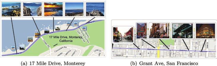
3:8     •      Y.-T. Zheng et al.

Fig. 4. Examples of POIs on roadside. A POI in (a) is visible from its nearby road and its photos are distributed along the road,
while a POI in (b) does not have good visibility from its nearby road and its photo distribution does not align well with the road.

   4.1.3 Visibility of a Roadside POI. A POI near a roadway is not necessarily a roadside POI. This is
because a roadside POI must be visible to travelers on the roadway. For example, a park with a fence
nearby a road might not be counted as a roadside POI, if the park is only visible through its entrance
and its fence blocks the rest of the view. The visibility of a roadside POI depends on two factors: (1)
its geospatial adjacency to the passing roadway, and (2) its alignment to the roadway direction. We
rely on a geocoding engine, that is, Goebase and Google Maps to enforce the geospatial adjacency, as
a POI would not be geocoded to a roadway far away. To tackle the alignment issue, we exploit the
dominant geospatial orientation of photos of a POI to determine its visibility to travelers on the road.
The premise is: if a POI is visible from a roadway, then its photos are highly probable to be distributed
along the roadway, as shown in Figure 4. Specifically, we utilize Principal Component Analysis (PCA)
[Joliffe 1986] to compute the dominant geospatial orientation of photos of a POI and determine its
alignment with a roadway. Principal component analysis is a commonly used mathematical procedure
to explain the variances in multivariate data. It transforms data into a set of uncorrelated variables,
which are called principal components. For photos in a POI, the first principal component accounts for
the direction of the maximal geospatial variation of photos, namely the dominant geospatial orienta-
tion. Specifically, we compute the dominant geospatial orientation of photos in a cluster Ci as follows.
Let Mi = [x y]T denote the geospatial coordinate of a photo in POI Ci and μi = E(Mi ) is the mean of
photos’ coordinates. The covariance matrix  i is computed as

                                                   i = E{(Mi − μi )(Mi − μi )T }.                                                      (3)

The eigenvectors eim with eigenvalues λim are the principal components of Mi , which can be solved by
using the eigenvalue decomposition method.

                                                     i · eim = λim · eim, m = 1, 2                                                     (4)

By sorting eigenvectors in decreasing order of their corresponding eigenvalues, we have the first and
second principal component of ei1 with eigenvalues λi1 and ei2 with eigenvalue λi2 , respectively. To make
POI Ci visible from a road , its dominant geospatial orientation of photos should be well aligned with
the road, as shown in Figure 4.
  Specifically, we measure the visibility of a POI Ci from a road  as follows. We have

                                          visibility(Ci , ) = cos αi · λi1 + sin αi · λi2 ,                                            (5)
ACM Transactions on Multimedia Computing, Communications and Applications, Vol. 9, No. 1, Article 3, Publication date: February 2013.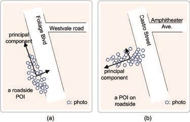
GPSView: A Scenic Driving Route Planner                 •      3:9

ALGORITHM 1: Discovering roadside POIs
 input: GPS-tagged photo set P = { p}
 output: roadside POIs {C}
 {Ci } = DBSCAN( photos P = { p})
 for all photo cluster Ci do
   validate Ci by number of uploaders
   if I({θ p}) ≥ εuploader , p ∈ Ci then
        = Geocoding(Ci );
       if visibility(Ci , ) ≥ εvisibility then
          label Ci as a roadside POI
       end if
   else
       discard Ci
   end if
 end for

  function {C} = DBSCAN( photos P = { p})
  input: GPS-tagged photo set P = { p}
  output: photo cluster {C}
  perform DBSCAN clustering on photo geospatial coordinates

                                                                                                                                    ei ·e
where αi is the angle between the POI dominant orientation and roadway direction, and cos αi = |ei1||e |
                                                                                                   1
with e as the direction vector of road . Intuitively, a POI with photos distributed along a roadway is
preferred, as a elongated POI is more suited for sightseeing on the drive.
  Furthermore, based on the numbers of photos and unique uploaders, the popularity of a POI Ci is
defined as
                                        popularity(Ci ) = log |Ci | + I({θ p, p ∈ Ci }),                                               (6)
where |Ci | is the number of photos in cluster Ci and I({θ p, p ∈ Ci }) is the number of unique uploaders
of all the photos in Ci . As a tourist may take a number of photos, we assume the number of tourists
and photos hold an exponential relation. Thus, we take log of the number of photos before summing it
up with the number of tourists. The sightseeing score of POI Ci near road  is then estimated jointly
by the popularity and visibility as follows.

                                  sightseeing(Ci ) = popularity(Ci ) · visibility(Ci , )                                              (7)

Algorithm 1 summarizes the procedure to discover roadside POIs.
  4.1.4 Building Scenic Roadway Models. Based on Definition 1, we represent a scenic roadway  as
a sequence < . . . , Ci , . . . > of adjacent POIs on its roadside. The construction of scenic roadway models
then becomes a grouping task. For each POI Ci along roadway  , we link it with its nearest neighbors.
This forms a directed graph, where vertices are POIs and edges are the driving distance computed
from a geocoding engine. After deleting edges above a threshold, the resulting subgraphs are scenic
roadway candidates. We use a heuristic method to decide the start and end point of a scenic roadway.
We first decode the road address of POIs and group them based on the corresponding roadways. Then,
we sort the POIs of the same roadway based on their street number. The POIs with the smallest and
largest street number are deemed to be the start and end point of the corresponding scenic roadway.
Note that a thoroughfare may have multiple segments of scenic roadways, if its POIs form groups that
are far apart from each other.
     ACM Transactions on Multimedia Computing, Communications and Applications, Vol. 9, No. 1, Article 3, Publication date: February 2013.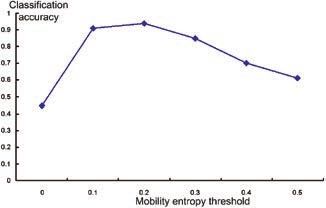
3:10 • Y.-T. Zheng et al.
The overall sightseeing experience is measured by the sum of sightseeing scores of individual POIs.
sightseeing() = popularity(Ci ) · visibility(Ci , ) (8)
Ci ∈
4.2 Planning Scenic Driving Route
Based on the discovered scenic roadways, we plan the scenic routes for motorists to have good sightsee-
ing experience on the drive. Given a starting point and a destination, we employ a geocoding engine,
like Google Maps, to compute the driving route with minimal traveling distance/time. Our task now is
to incorporate the scenic factor into driving route planning. The objective is to seek an optimal trade-
off between the sightseeing experience and the additional traveling distance caused by the detour.
Specifically, we formulate it as an optimization task in the framework of the Bellman-Ford algorithm
[Bellman 1958; Cormen et al. 2001].
Given a starting point s, an ending point e, and a set of scenic roadways R = < . . . , Ci , . . . > , we
first build a directed graph, in which the vertices comprise s, e and POIs Ci of all scenic roadways, and
the edges represent the trade-off between traveling distance and sightseeing experience between two
vertices as
dist(k, j), if j = r
w(k, j) = , (9)
dist(k, j) − β · sightseeing(C j ), otherwise
where dist(k, j) is the driving distance from vertex k to j computed from a geocoding engine, β is the
trade-off parameter between the driving distance and sightseeing quality, C j is the POI corresponding
to vertex j and sightseeing(C j ) indicates the sightseeing scores of traveling by POI C j , as defined in
Eq (8). Intuitively, Eq. (9) offsets the traveling distance with sightseeing on the way. With Eq. (9),
the scenic route planning is now cast as an optimization task towards the shortest geodesic of the
graph. Several solutions are available, such as Dijkstra’s algorithm [Dijkstra 1959] and the Bellman-
Ford algorithm [Bellman 1958]. We choose the Bellman-Ford algorithm, as it can handle edges with
negative weights with reasonably good efficiency. The computational complexity of Bellman-Ford runs
in O(|V | · |E|) time, where |V | and |E| are the numbers of vertices and edges, respectively.
5. EXPERIMENTS
5.1 Data
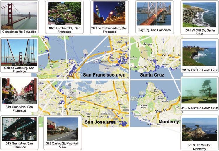
We test the proposed system on the region of northern California, including San Francisco, San Jose,
Santa Cruz and Monterey area, as shown in Figure 5. The GPS-tagged photos used were downloaded
from flickr.com and panoramio.com, with queries of local region names listed in Gazetteer, such as “San
Francisco”, “Sausalito”, “Mountain View”, “Monterey”, etc. In total, 831k photos were downloaded
and 84k of them were identified as tourist photos, as described in Section 4.1. Figure 5 shows the
distribution of photos used in this study.
5.2 Evaluation of Scenic Roadway Discovery
Here, we evaluate the process of the scenic roadway discovery. To build the scenic roadway, we first
select tourist photos and mine a set of roadside POIs in the local region.
5.2.1 Tourist Photo Selection. We construct a photo path of an uploader by concatenating his/her
photos in the order of photo time-stamps on a daily basis. We then compute the mobility entropy of
the photo path and classify it into a tourist or non-tourist photo path, based on the mobility entropy
threshold εmob. We determine the value of εmob, by analyzing its sensitivity to the tourist photo clas-
sification accuracy. First, we manually labeled a set of photo paths as the ground truth. We display
ACM Transactions on Multimedia Computing, Communications and Applications, Vol. 9, No. 1, Article 3, Publication date: February 2013.GPSView: A Scenic Driving Route Planner • 3:11
Fig. 5. Testing region and the distribution of GPS-tagged photos. One white dot represents a photo tagged to its location.
photos pertaining to a travel path and manually decide whether it is tourist or non-tourist based on
the visual content of tourism and sightseeing activities. For ambiguous photos, we simply regard them
as non-tourist photos. As manual annotation is laborious, we only label 1000 photo paths, of which 446
are tourist and 554 are not. Then we then compute the mobility entropy of each photo path and use
the mobility entropy threshold to classify them into a tourist and non-tourist photo path. We change
the threshold value εmob from 0.1 to 0.5 to evaluate the parameter sensitivity over the classification
accuracy. Figure 7 shows the tourist photo path classification accuracies at different values of thresh-
old. As shown, when εmob < 0.3, its sensitivity on accuracy is not obvious. However, when εmob > 0.3,
the accuracy drops drastically. This is because the higher threshold misclassified many tourist photo
paths as non-tourist ones.
5.2.2 Roadside POI Mining. To discover roadside POIs, we perform the DBSCAN clustering on
the geospatial coordinates of tourist photos, which yields a total of 1829 photos clusters. A reverse
geocoding is applied to decode the street address of these clusters. We then validate the resulting
photo clusters by the number of unique uploaders and compute the alignment between photos clusters
and their geocoded roadways. Finally, a total of 767 photo clusters are identified as roadside POIs with
reasonable visibility. Figure 6 displays the distributions of POIs on four maps (for better visual effect,
the plotting is done on four separate maps with a finer scale). As roadside POIs are fundamental to
build the scenic roadway database, we evaluate the accuracy of the identified POIs. The evaluation
is done by manually checking the photos pertaining to the POIs. If a considerable number of photos
of a POI present scenic, aesthetic, or interesting attributes, this POI is deemed valid. After careful
examination, 656 out of 767 POIs are found valid. Figure 6 displays some example photos of 12 valid
roadside POIs. Note that not all the POIs will be involved in a scenic roadway. This is because a scenic
roadway comprises a sequence of adjacent roadside POIs and an isolated POI will not be part of any
scenic roadways.
Next, we further evaluate the correctness of the quantitative visibility measure of a roadside POI
by PCA. Because we are not able to examine the scenery of roadways on site, we ask four respon-
dents to check the visibility of POIs in StreetView and give a visibility value ranging from 1 to 10 (10
means the best visibility). All respondents are not familiar with the target areas. We take this manual
annotation D as the estimated ground truth of POI visibility from the passing roadways. To evalu-
ate the correctness of visibility V generated by the proposed PCA-based method, we then measure
ACM Transactions on Multimedia Computing, Communications and Applications, Vol. 9, No. 1, Article 3, Publication date: February 2013.3:12 • Y.-T. Zheng et al.
Fig. 6. Distribution of roadside POIs on maps and example photos of 12 valid POIs. A blue dot on the map indicates a roadside
POI. For better viewing, please see the original color pdf file.
Fig. 7. Tourist photo path classification accuracies at different values of mobility entropy threshold εmob .
the correlations between them. If the PCA-based method works well, its resulting visibility measure
V should have strong linear correlation with the visibility values D annotated by the respondents.
Namely, they should agree statistically. Specifically, we utilize the Pearson’s product-moment coeffi-
cient [Rodgers and Nicewander 1988] to measure the correlation, as it is known to be sensitive to a
linear relationship between two variables. The correlation coefficient is defined as
cov(V, D) E[(V − μV )(D − μ D)]
ρ D,V = corr(V, D) = = , (10)
σV σ D σV σ D
where cov means covariance, σV and μV are the standard deviation and mean of V. The absolute value
of ρ D,V ranges from 0 to 1. ρ D,V = 1 means V and D have a perfect positive relationship, while ρ D,V = 0
means they are probabilistically independent. Our experiments give a ρ D,V of 0.76, indicating a strong
correlation between the visibility measure by the human annotation and the PCA-based method.
ACM Transactions on Multimedia Computing, Communications and Applications, Vol. 9, No. 1, Article 3, Publication date: February 2013.GPSView: A Scenic Driving Route Planner • 3:13
Fig. 8. Discovered scenic roadways. Each highlighted line represents a scenic roadway segment. For better viewing, please see
the original color pdf file.
5.2.3 Scenic Roadways Discovery. To discover scenic roadways, we use all the detected roadside
POIs, including those falsely identified. The intention is to make the generation of scenic roadways an
automatic process that does not require manual correction. A total of 55 scenic roadways are discov-
ered. Figure 8 illustrates the distribution of these scenic roadways on the maps. Similar to roadside
POIs, we evaluate the correctness of scenic roadways by checking their photos. After detailed exam-
ination, 6 out of 55 roadways are found not to present any scenic or visual attributes, such as the
Amphitheater Parkway in Mountain View. We attribute this false identification to the reason that
photos are not taken due to a visual or scenic factor of the roadway, but some event taking place there.
For example, the Amphitheater Parkway in Mountain View has an outdoor amphitheater that holds
concerts regularly. Many photos are taken outside or within the theater before or during the concerts.
We observe that the error rate (11%) in a scenic roadway is lower than the one (15%) in roadside POI.
This is because a scenic roadway comprises a sequence of adjacent roadside POIs and an isolated POI
will not be part of any scenic roadways.
The 49 correct scenic roadways consist of 2 highways (Cabrillo Highway and Big Sur Coast Highway)
and 47 local streets/roads. On average, the length of scenic roadways is 1.9km and the number of
roadside POIs per roadway is 5. Among the 49 correctly identified scenic roadways, 12 of them are
found to be natural scenery roadways, including the 17 Mile Drive in Monterey, W. CliffDrive in Santa
Cruz, etc., while the rest are cityscape roadways, including Market Street, Grant Ave in San Francisco,
etc. Figures 9(a), 9(b) and 1 show the examples of natural scenery and cityscape roadways.
ACM Transactions on Multimedia Computing, Communications and Applications, Vol. 9, No. 1, Article 3, Publication date: February 2013.3:14 • Y.-T. Zheng et al.
Fig. 9. Examples of discovered natural scenery and cityscape roadways and their scenery photos.
Table I. The Top 4 Most Popular Scenic Roadways
Roadway Region Length # of POIs
1 W Cliff Drive Santa Cruz 3.5km 17
2 Golden Gate Bridge San Francisco 1.2km 9
3 The Embarcadero San Francisco 2.3km 6
4 Market Street San Francisco 3.4km 7
200 100
150
100 50
0
Jan Feb Mar Apr May Jun Jul Aug Sep Oct Nov Dec Jan Feb Mar Apr May Jun Jul Aug Sep Oct Nov Dec
(a) Golden Gate Bridge, San Francisco (b) 17 Mile Drive, Monterey
Fig. 10. (a) and (b) show the monthly visit frequencies in Golden Gate bridge and 17 Mile Drive.
Most popular scenic roadways. According to Eq. (6), we estimate the popularity of scenic roadways,
based on their numbers of photos and unique uploaders. Table I lists the top 4 most popular roadways.
Figure 1 shows scenery photos of the “The Embarcadero in San Francisco” on the map. The “W Cliff
Drive” is a natural scenery roadway that offers a beautiful ocean view, while “The Embarcadero” in
San Francisco is a cityscape roadway that passes by several well-known tourist attractions, including
“the Bay Bridge”, “The Ferry Building”, “Pier 39”, etc.
5.3 Evaluation of Scenic Route Planning
As practical evaluation of a scenic driving route is difficult, we evaluate the performance of our route
planning system qualitatively through a user study. We test our system with 8 routing queries, as
summarized in Table II. Testing queries include travels within and between local regions with distance
ranging from 0.96km to 14.4km. We compare the scenic route generated by the proposed GPSView
with the shortest route generated by a commercial GPS service, that is, Google Maps. A total of 57
respondents with 43 male and 14 female with an average age of 26.5 are invited to the user study.
Among them, 3 respondents are familiar with San Francisco area, 12 have been there but not familiar,
and 42 of them have never been there. For each routing query, the respondents are shown photos along
the GPS and scenic route and their driving distance, respectively. The respondents are then asked to
answer the following 3 questions.
—Q1. Which route do you think has better scenery and will give a more pleasant driving journey?
—Q2. Which route do you prefer to drive on, considering both traveling distance and scenery?
—Q3. If a scenic route planner is available at your in-car GPS, are you willing to use it?
ACM Transactions on Multimedia Computing, Communications and Applications, Vol. 9, No. 1, Article 3, Publication date: February 2013.GPSView: A Scenic Driving Route Planner • 3:15
Table II. Testing Queries and Distances of Routes by GPS Service (Google Maps) and Scenic Routes
by GPSView
From To Scenic GPS
route route
227 Gharkey St, Santa Cruz, 2429 Mission Street, Santa Cruz 5.9km 2.4km
199 Geary St, San Francisco 1074-1076 Stockton St, San Francisco 1.8km 1.6km
218 Bay St, Santa Cruz 358 Swift St, Santa Cruz 4.2km 2.1km
1101 Francisco St, San Francisco 619 Chestnut St, San Francisco 1.28km 0.96km
173 Central Ave, Pacific Grove 300 Dickman Ave, Monterey 5.9km 2.4km
923 Sinex Ave, Pacific Grove 02 Corona Rd, Carmel 17.6km 12.2km
207 Swift St, Santa Cruz 560 Whispering Pines Dr, Scotts Valley 15.5km 12.6km
1721 Lombard St, San Francisco 1221 Bridgeway, Sausalito 32km 14.4km
Fig. 11. (a) and (b) show the scenic and GPS route from 1101 Francisco St, San Francisco to 619 Chestnut St, San Francisco,
respectively.
Fig. 12. Statistical results of the three questions in the user study. See Section 5.3 for details.
Figure 12 shows the results of the user study. As shown, 84.2% of respondents think that the scenic
routes by GPSView have better scenery than the shortest routes by GPS service, and therefore, can
offer a more pleasant driving experience. After considering both traveling distance and scenery, 61% of
respondents prefer to travel on the scenic routes over the shortest routes, despite the longer traveling
distance. This suggests that the scenery and sightseeing experience are important factors to determine
a driving route; and they can outweigh the additional traveling to some extent. We cross-checked the
route length and scenic-ness and found that people have a quite diverse preference on a scenery factor
and additional traveling. Some respondents picked the scenic route, even if it leads to a relatively long
traveling distance, while others are more sensitive to traveling distance than the scenery. Moreover,
78% of respondents show their willingness to have such a scenic route planner application in their
in-car GPS.
ACM Transactions on Multimedia Computing, Communications and Applications, Vol. 9, No. 1, Article 3, Publication date: February 2013.3:16 • Y.-T. Zheng et al. 5.4 Real-Time Responsiveness As the proposed system aims to provide real-time scenic route planning in in-car GPS devices, its response time is of paramount importance. The response time depends mainly on the complexity of the Bellman-Ford algorithm. The Bellman-Ford algorithm has the computational and memory space complexity of O(|V | · |E|) and O(|V |), respectively. Though the linear space complexity makes memory consumption insignificant, the running time could be cubic to the number of POIs. To ensure the real- time responsiveness of GPSView, we adopt a simple but effective approach, by only taking roadside POIs that are within a certain range of starting/ending points for route planning. Experiments show that the average running time for a route planning is 1.8 milliseconds on a 2.8GHz PC. As the pro- cessor speed of an ordinary in-car GPS device is about 200MHz [Garmin GPS Specification 2010], we expect the running time on a GPS device to be in the order of a hundred milliseconds (1.8×2800/200 = 25.2 milliseconds). 6. CONCLUSION We proposed an augmented GPS navigation system, GPSView, to plan driving routes with the scenic landscapes and sights. To do so, we first built a database of scenic roadways that afford vistas of no- table aesthetic, geological, cultural, and touristic features along roadsides. Specifically, we adapted an attention-based approach to exploit GPS-tagged photos for discovering scenic roadways. The premise is: a multitude of photos distributed along a roadway implies that this roadway is probably appealing and catches the public’s attention. By analyzing the geospatial distribution of photos, the proposed ap- proach ensures that the roadside scenic spots, or Points-Of-Interest (POIs), have good scenic qualities and visibility to travelers on the roadway. Finally, we formulated the scenic driving route planning as an optimization task towards the best trade-off between sightseeing experience and traveling distance. Testing in a northern California area showed that the proposed GPSView system can deliver promising results. Several issues are worthy of further investigation. First, when estimating the visibility of a roadside POI, this work does not take into account multi-lane highways, or parallel lanes/street that are sepa- rated by barriers. It is possible that a POI may have bad visibility from lanes on the other side of the roadway, especially when there are barriers in the middle The related lane and barrier information of roadways are the key information to tackle this issue. Second, the attractiveness of scenic sights, especially natural sceneries and landscapes, varies at different times and seasons. This dynamic factor needs to be taken into account for route planning. Fortunately, the time-stamps of photos provide a solution. By grouping photos according to its time taken, we can measure the number of tourist visits in a roadway at certain time, and therefore, pre- dict the sightseeing quality of a route in a time- and season-aware manner. Observation shows that the visits of natural scenery roadways, such as “17 Mile Drive” shown in Figure 11(a), are more subject to seasonal changes than cityscape roadways, like the “Golden Gate Bridge” as shown in Figure 11(b). Third, as the premise of the system is based on the geo-tagged photos, the lack of photos in some regions can be the major limitation to the system. For example, the system managed to detect only a segment of the “Big Sur Coast Highway”. Tourist maps and local knowledge are another information source to learn scenic roadways, which may complement the geo-tagged photos. Finally, while this study showed the subjects’ willingness to experience a GPS system that proposes scenic roadways as well as traditional paths, we must still evaluate the scenic roadway experience in practice. ACM Transactions on Multimedia Computing, Communications and Applications, Vol. 9, No. 1, Article 3, Publication date: February 2013.
GPSView: A Scenic Driving Route Planner                 •     3:17

REFERENCES
AGARWAL, S., SNAVELY, N., SIMON, I., SEITZ, S. M., AND SZELISKI, R. 2009. Building rome in a day. In Proceedings of International
  Conference on Computer Vision.
ASAKURA, Y. AND IRYO, T. 2007. Analysis of tourist behaviour based on the tracking data collected using a mobile communication
  instrument. Transp. Res. A: Policy Pract. 41, 7, 684–690.
BELLMAN, R. 1958. On a routing problem. Quart. Appl. Math. 16, 87–90.
CHIPPENDALE, P., ZANIN, M., AND ANDREATTA, C. 2009. Collective photography. In Proceedings of the Conference for Visual Media
  Production 0, 188–194.
CORMEN, T. H., LEISERSON, C. E., RIVEST, R. L., AND STEIN, C. 2001. Introduction to Algorithms. MIT Press.
CRANDALL, D. J., BACKSTROM, L., HUTTENLOCHER, D., AND KLEINBERG, J. 2009. Mapping the world’s photos. In Proceedings of the
  18th International Conference on World Wide Web. ACM, New York, 761–770.
DE CHOUDHURY, M., FELDMAN, M., AMER-YAHIA, S., GOLBANDI, N., LEMPEL, R., AND YU, C. 2010. Automatic construction of travel
  itineraries using social breadcrumbs. In Proceedings of the 21st ACM Conference on Hypertext and Hypermedia (HT ’10). ACM,
  New York, 35–44.
DIJKSTRA, E. W. 1959. A note on two problems in connexion with graphs. Numer. Math. 1, 269–271.
ELIAS, B. AND SESTER, M. 2006. Incorporating landmarks with quality measures in routing procedures. In Proceedings of the
  International Conference on Geographic Information Science. 65–80.
ESTER, M., KRIEGEL, H.-P., JÖRG, S., AND XU, X. 1996. A density-based algorithm for discovering clusters in large spatial databases
  with noise. In Proceedings of the Conference on Knowledge Discovery and Data Mining. ACM, 226–231.
GOESELE, M., SNAVELY, N., CURLESS, B., HOPPE, H., AND SEITZ, S. M. 2007. Multi-View stereo for community photo collections. In
  Proceedings of the IEEE Conference on Computer Vision.
HAO, Q., CAI, R., WANG, C., XIAO, R., YANG, J.-M., PANG, Y., AND ZHANG, L. 2010. Equip tourists with knowledge mined from
  travelogues. In Proceedings of the 19th International Conference on World Wide Web (WWW ’10). ACM, New York, 401–410.
HAO, Q., CAI, R., WANG, X.-J., YANG, J.-M., PANG, Y., AND ZHANG, L. 2009. Generating location overviews with images and
  tags by mining user-generated travelogues. In Proceedings of the 17th ACM International Conference on Multimedia. ACM,
  New York, 801–804.
HOCHMAIR, H. AND NAVRATIL, G. 2008. Computation of scenic routes in street networks. In Proceedings of the Geoinformatics
  Forum Salzburg.
HOCHMAIR, H. H. 2007. Optimal route selection with route planners: Results of a desktop usability study. In Proceedings of the
  Workshop on Advances in Geographic Information Systems.
JESDANUN, A. 2008. Gps adds dimension to online photos citation. http://www.physorg.com/news119889687.html.
JING, F., ZHANG, L., AND MA, W.-Y. 2006. Virtualtour: An online travel assistant based on high quality images. In Proceedings of
  the 14th Annual ACM International Conference on Multimedia. ACM, New York, 599–602.
JOLIFFE, I. T. 1986. Principal Component Analysis. Springer-Verlag.
KALOGERAKIS, E., VESSELOVA, O., HAYS, J., EFROS, A. A., AND HERTZMANN, A. 2009. Image sequence geolocation with human travel
  priors. In Proceedings of the IEEE International Conference on Computer Vision (ICCV ’09).
KAWAI, Y., ZHANG, J., AND KAWASAKI, H. 2009. Tour recommendation system based on web information and gis. In Proceedings of
  the IEEE International Conference on Multimedia and Expo. 990–993.
KENNEDY, L., NAAMAN, M., AHERN, S., NAIR, R., AND RATTENBURY, T. 2007. How flickr helps us make sense of the world: context and
  content in community-contributed media collections. In Proceedings of the International Conference on Multimedia. 631–640.
LEWA, A. AND MCKERCHERA, B. 2006. Modeling tourist movements: A local destination analysis. Ann. Tour. Res. 33, 2, 403–423.
LI, X., WU, C., ZACH, C., LAZEBNIK, S., AND FRAHM, J.-M. 2008. Modeling and recognition of landmark image collections using
  iconic scene graphs. In Proceedngs of the European Conference on Computer Vision. 427–440.
RATTENBURY, T., GOOD, N., AND NAAMAN, M. 2007. Towards automatic extraction of event and place semantics from flickr tags. In
  Proceedings of ACM SIGIR. ACM, New York, 103–110.
RODGERS, J. L. AND NICEWANDER, W. A. 1988. Thirteen ways to look at the correlation coefficient. Amer. Statist. 42, 59–66.
SANDER, J., ESTER, M., KRIEGEL, H.-P., AND XU, X. 1998. Density-Based clustering in spatial databases: The algorithm gdbscan
  and its applications. Data Min. Knowl. Discov. 2, 2, 169–194.
SNAVELY, N., SEITZ, S. M., AND SZELISKI, R. 2006. Photo tourism: Exploring photo collections in 3D. ACM Trans. Graph. 835–846.
SNAVELY, N., SEITZ, S. M., AND SZELISKI, R. 2008. Modeling the world from Internet photo collections. Int. J. Comput. Vis. 80, 2,
  189–210.

      ACM Transactions on Multimedia Computing, Communications and Applications, Vol. 9, No. 1, Article 3, Publication date: February 2013.
3:18 • Y.-T. Zheng et al. TORNIAI, C., BATTLE, S., AND CAYZER, S. 2007. Sharing, discovering and browsing geotagged pictures on the web. Tech. rep., HP Laboratories Bristol. WINTER, S. 2002. Modeling costs of turns in route planning. Geoinformatica 6, 363–380. YANAI, K., KAWAKUBO, H., AND QIU, B. 2009. A visual analysis of the relationship between word concepts and geographical locations. In Proceeding of the ACM International Conference on Image and Video Retrieval. ACM, New York, 1–8. ZHANG, J., KAWASAKI, H., AND KAWAI, Y. 2008. A tourist route search system based on web information and the visibility of scenic sights. In Proceedings of the International Symposium on Universal Communication. 154–161. ZHENG, Y., ZHANG, L., XIE, X., AND MA, W.-Y. 2009a. Mining interesting locations and travel sequences from gps trajectories. In Proceedings of the 18th International Conference on World Wide Web. ACM, New York, 791–800. ZHENG, Y.-T., ZHAO, M., SONG, Y., ADAM, H., BUDDEMEIER, U., BISSACCO, A., BRUCHER, F., CHUA, T.-S., AND NEVEN, H. 2009b. Tour the world: Building a web-scale landmark recognition engine. In Proceedings of the International Conference on Computer Vision and Pattern Recognition. Received September 2010; revised January 2012; accepted January 2012 ACM Transactions on Multimedia Computing, Communications and Applications, Vol. 9, No. 1, Article 3, Publication date: February 2013.
You can also read