Granger-causality between palm oil, gold and stocks (islamic and conventional): Malaysian evidence based on ARDL approach
←
→
Page content transcription
If your browser does not render page correctly, please read the page content below
Munich Personal RePEc Archive

Granger-causality between palm oil, gold
and stocks (islamic and conventional):
Malaysian evidence based on ARDL
approach

Othman, Nurhuda and Masih, Mansur

INCEIF, Malaysia, Business School, Universiti Kuala Lumpur,
Kuala Lumpur, Malaysia

20 February 2018

Online at https://mpra.ub.uni-muenchen.de/106777/
MPRA Paper No. 106777, posted 24 Mar 2021 15:22 UTC
Granger-causality between palm oil, gold and stocks (islamic and

conventional): Malaysian evidence based on ARDL approach

                                     Nurhuda Othman1 and Mansur Masih2

Abstract: This paper aims to ascertain the Granger-causality between Malaysian strategic

commodities (namely palm oil and gold prices) and stock markets (both conventional and

Islamic) using an ARDL or ‘Bounds Test’ The variables involved in this research are Crude

Palm Oil Price Malaysia (POM), Kijang Emas / Gold Price (KE), FTSE Bursa Malaysia KLCI (CI)

and FTSE Bursa Malaysia Emas Shariah Index (BMES). The empirical results tend to indicate

that Kijang Emas / Gold Price (KE) being the most exogenous leads the changes followed by

crude palm oil price, FTSE Bursa Malaysia KLCI (CI) and FTSE Bursa Malaysia Emas Shariah

Index (BMES) which is the most endogenous. We found there are causalities between stock

price and palm oil price. We also note, there are significant relationships between the

variables in the long run with a strong causal link between FTSE Bursa Malaysia EMAS Shariah

Index and FTSE Bursa Malaysia KLCI.

Keywords: Islamic stock market , Crude Palm Oil Price, Gold Price, ARDL

1
    INCEIF, Lorong Universiti A, 59100 Kuala Lumpur, Malaysia.

2 Corresponding author, Senior Professor, UniKL Business School, 50300, Kuala Lumpur, Malaysia.

Email: mansurmasih@unikl.edu.my

                                                                                                  0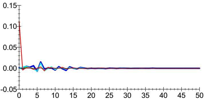
1. INTRODUCTION: THE ISSUE MOTIVATING THE STUDY

The palm oil, currently the world’s main vegetable oil crop, is characterized by a large

productivity and a long-life span, estimated more than 25 years. Malaysia is recognized as the

second largest exporter of palm oil behind Indonesia and together, both countries account

for 85% of the total global supply chain of palm oil. To date, Malaysia produced about 39% of

the world’s palm oil productions and 44% of world exports. Malaysia GDP agriculture sector

rebounded to a sturdy growth of 8.3% on a year-on-year basis s impelled by Oil Palm which

accelerated to a double-digit growth of 17.7%1. This industry accounts for approximately 6%

of the country’s gross domestic product (GDP) and is responsible for directly employing up to

600,000 people, ranging from low-skilled to high-skilled labors. Due to the significant

contribution of agriculture productivity, Malaysia government has allocated RM140 million

allocation for oil palm replanting, new plantings and promotion of palm oil exports. The

budget seeks to reinvigorate the commodity sector being the largest contributor of net

exports in 2018, spearheading economic progress above and beyond the Transformasi

Nasional 2050 agenda.

The second focus variables choose in this paper is gold where the investments are regarded

as an inflation hedge and safe asset for stock markets during the downturn periods (Baur and

Lucey, 2010). Gold is found positively correlated to inflation, a good instrument of inflationary

hedge (Bampinas and Panagiotidis, 2015). Such nature provides sense of certainty to the

investors during financial depressions and works as attractive alternative (Baur and

McDermott, 2010). The investment in gold can at least retains its purchasing power during

the periods of high inflation (Goodman, 1956). Gold can be used as portfolio diversifier since

1
    Press Release, Gross Domestic Products Q1 2017, Department of Statistics Malaysia.

                                                                                               1
it has low correlation with other assets therefore lowers the overall portfolio risk (Ciner et al.,
2013). Notably, the central banks also retain gold for diversification purposes and to
safeguard from economic uncertainties (Chen and Lin, 2014; Ciner et al., 2013; Kaufmann and
Winters, 1989; Kumar, 2014). Despite the positive role of gold investments in portfolio
diversification and hedging, market find volatility in gold prices has a negative impact on stock
markets. Lower volatility in gold prices indicates safe investment conditions (Baur, 2012).
The price of stock markets is impacted by various economic factors. However,
macroeconomic variables such as gold and oil are found to have profound impacts. In this
research instead of studying oil we wished to know the links of palm oil considering the
position of Malaysia as palm oil producer in the world. Previous studies on this topic
(Beckmann and Czudaj, 2013; Kanjilal and Ghosh, 2014; Shahbaz et al., 2014; Wang et al.,
2011) have mainly analyzed the stock, gold and oil linkages in a linear setting. Anoruo (2011)
argues the practicality of linear regression than the non linear noting the nature of variable
discussed.
2. LITERATURE REVIEW
Hussin et.al. (2013) concluded in their findings that Islamic stock returns were not co-
integrated with strategic commodities in the long run. From the Granger causality viewpoint,
it was observed that there was a bi-directional causality relationship between Islamic stock
returns with oil prices. On the other hand, the FBMES was not affected by the gold prices or
vice versa. Therefore, it can be concluded that, among strategic commodities, only oil price
variables will affect the Islamic stock return in the short run in Malaysia. They further
concluded that Kijang Gold Price is not a valid variable for predicting changes in Islamic share
prices.
2While for the palm oil study many studies have been conducted to study the investigation
with crude oil. Since there is a lack of literature that includes palm oil in this nexus, we will be
extrapolating the ideologies behind those applied to crude oil onto palm oil. Even if there are
studies on palm oil they are using more advanced method of nonlinear ARDL. Haron, et.al.
(2015) did a volatility analysis on palm oil where according to them, the Malaysian CPO
commodity market is volatile. However, the study does not detail out the factors affecting
the volatilities.
Therefore, in this section, we will be discussing the underlying theoretical framework and
review the existing body of knowledge.
3. THE OBJECTIVE OF THE STUDY
(i) To know the Granger-causal direction between Malaysia palm oil, Gold and Malaysian
stock market (both Islamic and Conventional)?
(ii) Can palm oil price be used as inflation hedge for stock price fluctuation? If yes, is it
better than Kijang Emas (Gold)?
4. THEORETICAL UNDERPINNINGS
The dynamic relationship that exists between share returns and macroeconomic variables
have been extensively discussed, the basis of these studies being the use of models which
state that share prices can be appropriately written as the expected discounted cash flow. It
can be said, then, that share price determinants are the required rate of return and expected
cash flows (Elton and Gruber, 1991).
3Malaysian crude palm oil has been a major export commodity and contributing signifcantly
to the Malaysian economic development. PALM OIL is an agricultural commodity traded in a
standardized exchange – Bursa Malaysia derivatives Berhad (BMdB). In addition, since
Malaysia host the largest and third largest public listed palm oil companies in the world, i.e.
Sime Darby Berhad and Felda Global Ventures Holdings Berhad and other large companies
control up to 60% of Malaysia’s palm oil plantations. Noting on the same we then form
hypothesis that palm oil prices would have a significant impact on the Malaysian stock
market. In this research, the stock market of Islamic and conventional is differentiated
learning the player in Islamic stock can participate the conventional market without shariah
restriction.
Crude palm oil and gold are strategic resources that are largely used in various national
economic activities and in national security. Due to this, we include the 4the variable of Kijang
Emas (Gold) to see the causality to the model. Large fluctuations in crude palm oil and gold
markets may lead to increased price volatility, which affects price stabilization policies and
imposes more challenges on market participants (producers, consumers, and investors), who
often try to predict the future prices of the commodities.
5. THE METHADOLOGY & DATA USED
DATA
A total of two strategic commodities variables and two stock indices monthly data duration
from July 2017 – Nov 2017 representing Islamic and Conventional have been used in the
analysis. The definitions of each variable and sources described as below:
4Table.1: Definitions and Source of Variables
No Variable Description Source
1. KE Kijang Emas, Gold Price BNM website
2. POM Crude Palm oil price (Malaysia) Thompson Reuters
3. BMES FTSE Bursa Malaysia Emas Shariah DataStream
4. CI FTSE Bursa Malaysia KLCI
METHODOLOGY
In hypothesis testing lead – lag relationship, researcher may choose to adopt the either cross-
sectional or time-series approaches. The cross-sectional approach has a major shortcoming
in testing lead-lag relationships because they are not appropriate in capturing the dynamics
of the variables involved. Moreover, cross-sectional studies are underlying with many
assumptions that is not realistic. In findings the lead – lag relationship, time series study to
individual country is more suitable.
Although the time-series techniques are an improvement to cross-sectional studies in testing
Granger causality, they are still limited where the error correction/variance decompositions
methods are based on the estimates of the cointegrating vectors, which are a theoretical in
nature. Such limitation then taken care by the development of ARDL technique. The ARDL
bounds testing approach is more appropriate compared to those traditional cointegration
approaches. The approach avoids endogeneity problems and the inability to test long run
relationships of variable associates with the traditional Engel-Granger method. Both short run
and long run parameters are calculated simultaneously and the ARDL approach can be used
regardless of whether the data are integrated of order I(0) or I(1). Narayan (2005) argues that
the ARDL approach is superior in small samples to other single and multivariate cointegration
5methods. The following 5 regressions are constructed without any prior information as to the
direction of the relationship between the variables. The ARDL model specifications of the
functional relationship between palm oil (POM), Kijang Emas (Gold) (KE), Carbon
Emission(CO), FTSE Bursa Malaysia Emas Shariah (BMES) and FTSE Bursa Malaysia KLCI (CI)
can be estimated below:
The relationships between the four variables are analyzed using econometric tools namely;
1) Unit Root Test
2) Auto Regressive Distributed Lag (ARDL) - a more advance cointegration test usable even if
the variables are stationary at different levels I(0) and I(1).
3) Variance Decomposition (VDC) - to rank the leading variables or the most independent.
4) Impulse Function Response (IRF) - a test of their inter-temporal linkages, and
A) UNIT ROOT TEST
In time series, variables a non-stationary in their raw form. That means, choosing these
variables to perform an ordinary regression will produce us misleading results. The below is
ADF test where we test the stationarity of the variables selected from the analysis all the
variable are stationary at 1st difference. Hence, we proceed our test to VAR lag order.
6Table 2: Augmented Dickey–Fuller (ADF) tests table
VARIABLE ADF VALUE T-STAT. C.V. RESULT
ADF(3)=SBC 66.0318 - 3.659 - 3.448 Stationary
LPOM
ADF(3)=AIC 74.3691 - 3.659 - 3.448 Stationary
LOG FORM
ADF(3)=SBC 147.8993 - 2.517 - 3.448 Non-Stationary
LCI
ADF(5)=AIC 156.6267 - 3.048 - 3.448 Non-Stationary
ADF(3)=SBC 144.8054 - 3.114 - 3.448 Non-Stationary
LBMES
ADF(3)=AIC 153.1428 - 3.114 - 3.448 Non-Stationary
ADF(1)=SBC 83.4301 -1.5901 -3.4478 Non-Stationary
LKE
ADF(1)=AIC 88.9883 -1.5901 -3.4478 Non-Stationary
VARIABLE ADF VALUE T-STAT. C.V. RESULT
ADF(2)=SBC 63.4894 - 4.603 - 2.886 Stationary
DPOM
1ST DIFF. FORM
ADF(2)=AIC 69.0308 - 4.603 - 2.886 Stationary
ADF(2)=SBC 153.4094 - 6.247 - 2.886 Stationary
DCI
ADF(2)=AIC 147.8680 - 6.247 - 2.886 Stationary
ADF(2)=SBC 142.9747 - 5.802 -2.8859 Stationary
DBMES
ADF(2)=AIC 148.5161 - 5.802 -2.8859 Stationary
ADF(1)=SBC 81.895 -7.786 -2.8859 Stationary
DKE
ADF(1)=AIC 86.0511 -7.786 -2.8859 Stationary
Next we test the variables to confirm that none of the variables is I(2) using Augmented DF
test and observed that variables are I(1) when we checked at level form and I(0) at first
difference. Using VAR order in serial correlation is a common feature and useful where
stationary time series move together. We need to determine the order of the Vector auto
regression (VAR), how many lags to be used. The result below shows that AIC recommends
order of 3 while SBC favors 0 lag.
7Table 3: VAR Lag order table
Adjusted LR
Order LL AIC SBC LR test
test
6 742.1328 642.1328 503.5986 - -
5 732.5955 648.5955 532.2268 CHSQ(16)=19.0745[.265] 15.0333[.522]
4 719.6197 651.6197 557.4164 CHSQ(32)=45.0263[.063] 35.4868[.307]
3 711.2177 659.2177 587.1799 CHSQ(48)=61.8302[.087] 48.7306[.443]
2 693.7008 657.7008 607.8285 CHSQ(64)=96.8640[.005] 76.3419[.139]
1 678.1416 658.1416 630.4348 CHSQ(80)=127.9824[.001] 100.8675[.057]
0 643.7005 639.7005 634.1591 CHSQ(96)=196.8647[.000] 155.1561[.000]
Choice Criteria
AIC SBC
Optimal order 3 0
But given the conflicting results we checked for serial correlation in each variable and
obtained the following results as below:
Table 4: Serial Correlation tests table
VARIABLE Chi-Sq P-Value Implication at 5%
DPOM 0.450 No serial correlation
DCI 0.003 There is serial correlation
DBMES 0.001 There is serial correlation
DKE 0.045 There is serial correlation
As evident from the above results, there is autocorrelation in 3 out of 4 variables. Based on
result we choose AIC since tends to produce the most accurate for bigger sample size for
which SBC is more accurate for lower than 120 (Ivanov and Kilian, 2005). Noting most of our
8variables suffered auto – correlation problem, we choose 3 lags in order to eliminate the auto
correlation problem.
B. TESTING COINTEGRATION
There are numbers of co-integration test that we learnt which is Engle – Grager, Johansen
and ARDL. However, there are benefits of ARDL that suitable for this research purpose i.e it
works better for small sample size. Due to that we decide to proceed with ARDL a model was
introduced by Paseran et al. (2001) in order to incorporate stationary variables I(0) and non
stationary I(1) variables in same estimation. Previously OLS test is used with assumption that
variables are all at I(0) level in time series data but obviously they are not held constant as
most of them changing all the time.
AUTO REGRESSIVE DISTRIBUTED LAG (ARDL)
To empirically analyze the dynamic relationship of multi dimensions variables, we use ARDL
co-integration procedure developed by Pesaran et al. (2001) due to a few reasons.
i) It is a unique technique against other multivariate cointegration like Johansen and
Juselius (1990) where it allows co-integrating relationship to be estimated by OLS
once the lag order is selected.
ii) It doesn’t require the pre-testing of the variables in finding unit root.
iii) The error correction method integrates the short run dynamics with long run
equilibrium without losing long run information (Joshi, 2015).
9The ARDL procedure involves two stages. First, testing the existence of the long-run relation
between the variables and secondly, estimating the coefficients of it.
In its basic form, an ARDL model looks like this:
yt = β0 + β1yt-1 + .....+ βpyt-p + α0xt + α1xt-1 + α2xt-2 +.....+ αqxt-q + εt
where εt acted as random ‘disturbance’ term.
When we perform the ‘Bound Testing’, we are testing the absence of a long-run equilibrium
relationship between the variables with H0 is there is no-lung run relationship. ARDL technic
supply bound on the critical values with lower and upper number on the critical values. If the
computed F statistic falls below the lower bound, we can conclude that the variables are I(0)
so there is no-cointegration and if it exceeds the upper bound, then we conclude that we have
co-ingetration. If the F-statistic falls between the bounds, the test is inconclusive.
The null hypothesis for the F-test is H0 = 1 = 2 = 3 = 4 =5 = 0 which indicates there is no
long-run co-integration among variables, against the alternative hypothesis that long run co-
integration does exist among variables ( H1 = 1 ≠ 2 ≠ 3 ≠ 4 ≠ 5 ≠ 0 )
Given 4 variables are tested in this paper, according to the F-table, the lower bound is at 3.063
for I(0) and the upper bound I(1) is at 4.084. The result below shows there are 2 of the
variables have co-integration in the long run which is stock prices of conventional and Islamic.
This is probably due to the variables’ observation taken by monthly data.
10Table 5: ARDL co-integration tests table
VARIABLES F-STATISTIC IMPLICATIONS
DPOM 3.9987 NO CO-INTEGRATION
DBMES 4.9390 THERE IS CO-INTEGRATION
DCI 4.3540 THERE IS CO-INTEGRATION
DKE 3.1533 NO CO-INTEGRATION
LONG RUN STRUCTURAL MODELLING (LRSM)
Based on our result that there is one co-integration with assumption that there must be at
least more than one variable co-integrated in the long, we move to the long run equilibrium
relationship between the variables. Here we attempt to quantify the theoretical relationship
among the variables in order to compare our statistical findings with theoretical (or intuitive)
expectations. We found that only one variable that is Brent oil is not significant while others
are very significant. We also found that only Unit Trust growth will affect positively to
FTSEBMS while others are negatively correlated. This support our intuition that the Unit Trust
growth has a significant impact on Shariah Index. Other variables like inflation and USD/MYR
exchange will have a negative impact with an increase of one percent.
Table 6: LRSM table
Estimated Long Run Coefficients using the ARDL Approach
ARDL(4,0,4,0) selected based on Akaike Information Criterion
*******************************************************************************
Dependent variable is LPOM
110 observations used for estimation from 2007M12 to 2017M1
*******************************************************************************
Regressor Coefficient Standard Error T-Ratio[Prob]
LCI 6.5556 4.3991 1.4902[.139]
LBMES -5.2216 3.7875 -1.3786[.171]
LKE -0.15222 0.25045 -.60779[.545]
C 52.5939 32.6247 1.6121[.110]
*****************************************************************************************************
11The result can be written as below:
LPOM = 52.59 + 6.5556.LCI** – 5.2216LBMES** – 0.1522LKE
ERROR CORRECTION MODEL
In error-correction term the coefficient of ECM(-1) is the most important as the result must
falls between -1 and 0 to prove that there exists partial adjustment . A value smaller than -1
indicates that the model over adjusts in the current period while a positive value implies that
the model moves away from equilibrium in the long-run.
In our result on the et-1 we notice that the coefficient of the error-correction term is negative
(-0.10504) and very significant (0.003). The magnitude of this coefficient implies that nearly
11% of any disequilibrium between the variables is corrected within one period or one month.
The ECM reported as equation below.
Table 6: Error Correction Model table
Error Correction Representation for the Selected ARDL Model
ARDL(4,0,4,0) selected based on Akaike Information Criterion
*******************************************************************************
Dependent variable is dLPOM
110 observations used for estimation from 2007M12 to 2017M1
*******************************************************************************
Regressor Coefficient Standard Error T-Ratio[Prob]
dLPOM1 0.31429 0.095496 3.2912[.001]
dLPOM2 -0.033706 0.098231 -.34313[.732]
dLPOM3 0.35672 0.099551 3.5833[.001]
dLCI 0.68861 0.49578 1.3889[.168]
dLBMES 0.46297 0.45954 1.0075[.316]
dLBMES1 -0.26894 0.17984 -1.4954[.138]
dLBMES2 0.051883 0.17819 .29116[.772]
dLBMES3 -0.32257 0.16751 -1.9256[.057]
dLKE -0.01599 0.026449 -.60454[.547]
dC 5.5246 3.7542 1.4716[.144]
ecm(-1) -0.10504 0.034983 -3.0026[.003]
*******************************************************************************
12VARIANCE DECOMPOSITION (VDC)
Variance decomposition finds out to what extent shocks to specified variables are explained
by other variables in the system. Variance decomposition measures the amount of forecast
error variance in a variable that is explained by innovations or impulse in it and by the other
variables in the system. For instance, it discloses to what proportions of the changes in a
variable can be associated to changes in the other lagged explanatory variables. Moreover, if
a variable explains most of its own shock i.e exogenous, then it does not permit variances of
other variables to assist to its explanation and is therefore said to relatively exogenous. There
are two types of VDC that is orthogonalized and generalized. The difference between these
two is that in orthogonalized forecast error variance decomposition, the amount of
percentage of the forecast error variance of a variable which is counted for by the innovation
of another variable in the VAR will sum to one across all the variables. On the other hand,
generalized forecast error VDC permits one to make robust correlation of the strength, size
and persistence of shocks from one equation to another (Payne, 2002) and for that reason
we employ generalized VDC as opposed to orthogonalized VDC.
The generalized VDC analysis shows that variable that is explained by its own past variations
will be the most exogenous. According the results below, the ranking of variables according
to the degree of exogeneity.
13Table 7: Variance Decomposition Table
HORIZON DPOM DCI DBMES DKE TOTAL SELF-DEP RANKING
DPOM 12 48.64% 25.89% 24.05% 1.42% 100.00% 48.64% 2
DCI 12 17.47% 41.74% 37.95% 2.83% 100.00% 41.74% 3
DBMES 12 17.30% 40.48% 39.95% 2.26% 100.00% 39.95% 4
DKE 12 7.01% 5.14% 4.37% 83.47% 100.00% 83.47% 1
HORIZON DPOM DCI DBMES DKE TOTAL SELF-DEP RANKING
DPOM 36 48.58% 25.82% 23.95% 1.65% 100.00% 48.58% 2
DCI 36 17.66% 41.60% 37.76% 2.97% 100.00% 41.60% 3
DBMES 36 17.50% 40.35% 39.73% 2.42% 100.00% 39.73% 4
DKE 36 7.44% 5.32% 4.53% 82.71% 100.00% 82.71% 1
HORIZON DPOM DCI DBMES DKE TOTAL SELF-DEP RANKING
DPOM 48 48.58% 25.82% 23.95% 1.65% 100.00% 48.58% 2
DCI 48 17.66% 41.60% 37.76% 2.97% 100.00% 41.60% 3
DBMES 48 17.50% 40.35% 39.73% 2.42% 100.00% 39.73% 4
DKE 48 7.44% 5.32% 4.53% 82.71% 100.00% 82.71% 1
Conventional Islamic Stock
Gold Palm Oil
Stock Price Price
Most Most
Exogenous Endogenous
From the above results, we can make the following key observations:
1. The Generalized VDC result shows that Kijang Emas (Gold) price is the most exogenous
variable followed by palm oil, conventional stock price and lastly islamic stock price.
The ranking is consistent through the period of 50 observations.
2. Kijang Emas (Gold) Price responded strongly to its own shock around 83% with very
minimal contribution from other variables. This variable also does not contribute
much when we shock the rest of the variables, mainly less than 3%. We find this
14contradict with findings of Baur 2012, where it mentioned the volatility in gold prices
has a negative impact on stock markets. Lower volatility in gold prices indicates safe
investment conditions. This findings however inline with Hussin et.al (2013) where
concluding Kijang Gold Price is not a valid variable for the purpose of predicting
changes in Islamic share prices.
3. The palm oil price change around 50% to its own innovation. From our observation,
this variable shock change also contributed by stock price, conventional and Islamic,
sharing nearly equal portion of 25% where the conventional always take the lead.
4. FTSE Bursa Malaysia KLCI change is contributed by its own innovative shock around 42
per cent for the whole period of 50 observations. This variable can be predicted by
FTSE Bursa Malaysia Shariah Emas and palm oil price that contributed around 38% per
cent and 18 per cent across all period observations respectively.
5. FTSE Bursa Malaysia Emas Shariah change is observed contributed more by FTSE Bursa
Malaysia KLCI which normally stood at 41% more than itself around 40%. Palm oil price
that contributed marginally at 18 per cent across all period observations respectively.
The result of exogeneity between palm oil and kijang emas (gold) show that the former is
more exogenous than the latter, followed by FTSE Bursa Malaysia KLCI and FTSE Bursa
Malaysia Emas Shariah position at the last as the most endogenous.
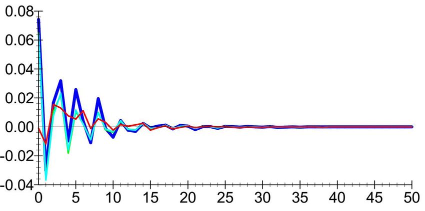
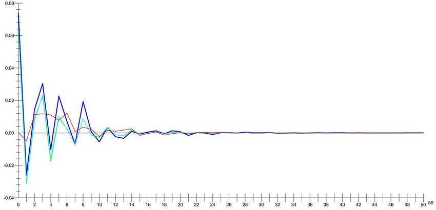
IMPULSE RESPONSE FUNCTIONS (IRF)
To examine the dynamics of exogenous variables and their impact, we employ Impulse
Response Function (IRF) to illustrate the dynamic patterns of all variables especially FTSE
Bursa Emas Shariah Index and our focus variable, Islamic unit trust. The IRF are calculated
15over a 50-monthly time horizon. The initial shock in a variable is set to be equal to one
standard error of innovation; the vertical axis in the figures reports the approximate
percentage change in other variables in response to a one-percentage shock in issue. The
results are shown in figure below. The Impulse Functions Response (IRF) essentially produce
the same information as the VDC, except that they can be presented in graphical form.
Crude palm oil price (Malaysia)
FTSE Bursa Malaysia Emas Shariah
16FTSE Bursa Malaysia KLCI
Kijang Emas, Gold Price
176. CONCLUSION
This study was conducted with the main goal of ascertaining the co-movement between
palm oil price returns with Kijang Emas (Gold) and the index returns of two stock indices,
namely FTSE Bursa Malaysia Emas Shariah and FTSE Bursa Malaysia KLCI. Monthly data from
Nov 2007 up until Nov 2017 where we apply time series econometrics technics of unit root,
Auto Regressive Distribution Lags (ARDL) or ‘Bound Test’, Variance Decomposition (VDC) to
study the long run relationship among the variables and discern their dynamic causal
interactions.
From the result we conclude, firstly, the Kijang Emas / Gold Price (KE) – who own the most
exogeneity lead the changes followed by crude palm oil price, FTSE Bursa Malaysia KLCI (CI)
and FTSE Bursa Malaysia Emas Shariah Index (BMES) having the most lag. We also found
there are causalities between stock price and palm oil price.
However, we found no causality between gold and the other variables where we observed
while the variable Kijang Emas (Gold) is the most exogenous, but it does not contribute to
the change of the other 3 variables. The ranking is consistent throughout the 50 months of
observation. It also shows that each time series describes the prevalence of its own values
with clear bi-directional causality. Gold stood strong on its own innovation and does not
affect the other variables when changes are made to the other variables, implying the
features of good hedging alternative. Learning from the power of exogeneity owned by
Kijang Emas (Gold) and the negative correlation towards the rest of variables, having Kijang
Emas (Gold) on the portfolio mix could be a good idea.
We found that both the conventional and Islamic stock markets are strongly correlated with
each other. They do contribute to the change of palm oil, but the change of palm oil is mostly
contributed by innovation made to itself. The co-movements of these stock markets towards
18price of palm oil were similar in nature. Therefore, for the portfolio strategic management,
we humbly suggest to investor to carefully observe the mix of palm oil in their portfolio.
Our empirical results are practically useful for policy makers who have been using palm oil
and gold and as instruments to manage stock price change in Malaysia. The portfolio
manager can be benefitted most. The results are also valuable to investors and commodity
hedgers in reducing the risk of their portfolios. With the causality result this can be applied
as risk management tools, market participants can use them as derivatives in hedging the
risk in the gold, crude palm oil, and Malaysian stock markets investment and in equity-
commodity portfolio management.
Nevertheless, this study may not be entirely comprehensive. In this study, we did not
consider another significant event of boycott held by other countries on the palm oil based
on the accusation that this industry is violating the sustainability and ecosystem of our earth.
Future studies may include the horizon of this event started and learn how does this
sentiment affects the Malaysia market. This study is important for us to know the
vulnerabilities of palm oil market in Malaysia and neighbouring ASEAN and Asian region as
this is where the demand for palm oil is high. Lastly, we sincerely hope that this study and its
findings would be able to contribute to the growing importance of the palm oil industry as
knowledge in this nexus is still relatively scarce. Any shortcomings and unintended errors in
this study reflect the author alone.
197. REFERENCES
Anoruo, E., (2012). Testing for linear and nonlinear causality between crude oil price
changes and stock market returns. International Journal of Economic Sciences and
Applied Research, 4 (3), 75–92.
Bampinas, G. and Panagiotidis, T., (2015). Are gold and silver a hedge against inflation?
Two century perspective. International Review of Financial Analysis, 41, 267–276.
Baur, D.G. and Lucey, B.M., (2010). Is gold a hedge or a safe haven? Analysis of Stocks,
Bonds and Gold, Financial Review,. 45 (2), 217–229
Baur, D.G. and McDermott, T.K., (2010). Is gold a safe haven? International evidence.
Journal of Banking and Finance, 34 (8), 1886–1898
Beckmann, J. and Czudaj, R., (2013). Gold as an inflation hedge in a time-varying
coefficient framework. North American Journal of Economics and Finance, 24, 208–
222.
Bouri, E., Jain, A., Biswal, P. C., and Roubaud, D. (2017). Cointegration and nonlinear
causality amongst gold, oil, and the Indian stock market: Evidence from implied
volatility indices. Resources Policy, 52, 201-206.
Chen, A.S. and Lin, J.W., (2014). The relation between gold and stocks: an analysis of
severe bear markets. Applied Economics Letters, 21 (3), 158–170.
Ciner, C., Gurdgiev, C. and Lucey, B.M., (2013). Hedges and safe havens: an
examination of stocks, bonds, gold, oil and exchange rates. International Review of
Financial Analysis,. 29, 202–211
Elton, E.J. and M. Gruber. (1991), Modern Portfolio Theory and Investment Analysis,
Fourth Edition, New York: John Wiley & Sons.
20Goodman, B., (1956). The price of gold and international liquidity. Journal of Finance,
11 (1), 15–28.
Hussin, M. Y. M., Muhammad, F., Razak, A. A., Tha, G. P., and Marwan, N. (2013).
The link between gold price, oil price and islamic stock market: experience from
Malaysia. Journal of Studies in Social Sciences, 4(2), 161-182.
Kaufmann, T.D. and Winters, R.A., (1989). The price of gold: a simple model. Resources
Policy, 15 (4), 309–313.
Raza, N., Shahzad, S. J. H., Tiwari, A. K., and Shahbaz, M. (2016). Asymmetric impact
of gold, oil prices and their volatilities on stock prices of emerging markets, Resources
Policy, 49, 290-301.
Razak, R., and Masih, M. (2017). The links between crude palm oil, conventional and
Islamic stock markets: evidence from Malaysia based on continuous and discrete
wavelet analysis, MPRA paper, Number 79717.
Shahbaz, M., Tahir, M.I., Ali, I. and Rehman, I.U., (2014). Is gold investment a hedge
against inflation in Pakistan? A co-integration and causality analysis in the presence of
structural breaks. North American Journal of Economics and Finance, 28, 190–205.
Wang, K.M., Lee, Y.M.and Thi, T.B.N., (2011). Time and place where gold acts as an
inflation hedge: an application of long-run and short-run threshold model. Economic
Modelling,. 28 (3), 806–819
Woittiez, L. S., van Wijk, M. T., Slingerland, M., van Noordwijk, M., and Giller, K. E.
(2017). Yield gaps in oil palm: A quantitative review of contributing factors. European
Journal of Agronomy, 83, 57-77.
21You can also read