Gravitational Lensing as a Cosmological Tool - Gravitational lensing by the Sun was an early observational success of General Relativity. Today ...
←
→
Page content transcription
If your browser does not render page correctly, please read the page content below
Gravitational Lensing as a
       Cosmological Tool

       Gravitational lensing by the Sun was an early
       observational success of General Relativity. Today,
       gravitational lensing is one of the most powerful
       observational tools used in Cosmology.

                                                             1
2. Jul 2021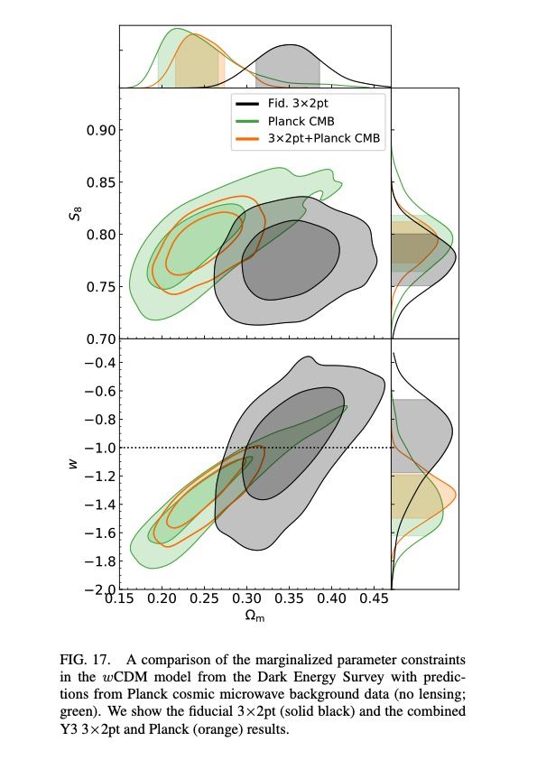
Overview
n    Light Deflection

n    Simple Lens Models

n    Properties of Thin Lenses

n    Observations of gravitational lensing

    2. Jul 2021         Cosmology and Structure Formation - Mohr - Lecture 7   2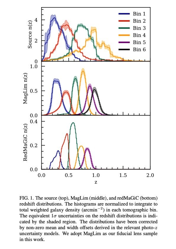
Light deflection
n    Bending angle of light passing by point mass can be calculated classically
       n   In small bending angle approximation the accelerations parallel to the photon direction
           of travel cancel, so we don’t have to confront changes to the speed of the photon! J
       n   One simply considers the accelerations perpendicular to the line of site- along z axis

                              DLS                                DL

    2. Jul 2021                  Cosmology and Structure Formation - Mohr - Lecture 7           3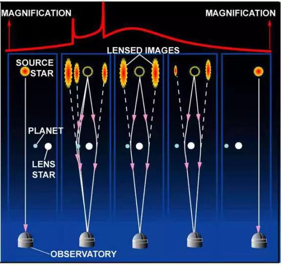
Bending Angle
n    Bending angle is time or line integral over gradient in potential
                                vz 1          dΦ      1          dΦ
                          α=      =
                                vl vl
                                          ∫   dz
                                                 dt = 2
                                                     vl
                                                             ∫   dz
                                                                    dl

                                                                              Note that neither the
n    This expression is clearly reflected in the GR result                    mass of the deflected
                                     2                                        particle nor the energy
                                 α = 2 ∫ ∇ ⊥Φ dl                              of the deflected
                                     c
                                                                              photon appears:
n    For a point mass we can write the potential
                                                                                   lensing does not
                                                 −GM                               introduce color
                                   Φ (l, z ) =                                     dependent effects
                                                  l 2 + z2

n    And the spatial gradient along z is          dΦ     GMz
                                                     =           3
                                                  dz (l 2 + z 2 ) 2
    2. Jul 2021            Cosmology and Structure Formation - Mohr - Lecture 7                   4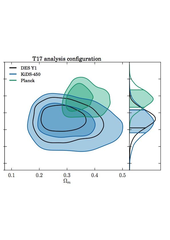
Gravitational Deflection
n    Bending angle is time or line integral over gradient in potential
                                                                                       ∞
              ∞                       ∞                       $                    '
           2        GMz          4GMz        dl          4GMz &          l         ) = 4GM
       α = 2 ∫ dl           3  =      ∫             3  =                        1
           c −∞ (l 2 + z 2 ) 2    c 2 0 (l 2 + z 2 ) 2    c 2 & z 2 (l 2 + z 2 ) 2 )    c2 z
                                                              %                    (0
n    For an impact parameter b we then recover the famous result
                                             4GM 2RS
                                       α=      2
                                                 =
                                              cb   b
              where Rs is the Schwarzschild radius

n    Thus, the bending angle for the sun (M=2x1030kg, Rs~3km) at the
     impact parameter equal to the radius of the sun (7x10⁵km) is:
                                             α o,Ro = 1.7"

    2. Jul 2021                 Cosmology and Structure Formation - Mohr - Lecture 7           5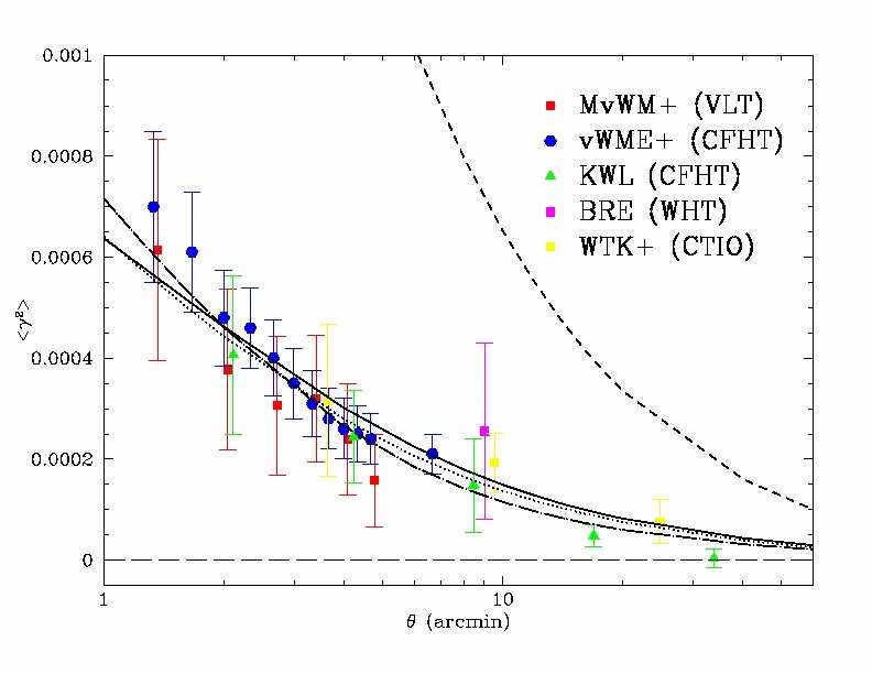
Geometry of Lensing Event
n    Key parameters of lensing event
     include:
       n   Angles:
              n   a: bending angle
              n   qI: angle between lense and image
              n   qS: angle between lense and source
       n   b: distance of closest approach
       n   Distances:
              n   DLS distance lense to source
              n   DL distance observer to lense
              n   DS distance observer to source

n    Bending angle is geometrically related
                                                                              α DLS = DS (θ I − θ S )
     to physical distances and to angles that
     can be measured on the sky                                                       DS
                                                                                α=        (θ I − θ S )
                                                                                      DLS

    2. Jul 2021                      Cosmology and Structure Formation - Mohr - Lecture 7                6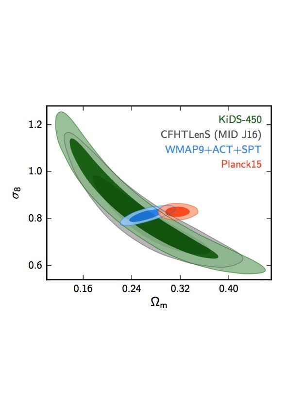
Lensing Amplification of Magnification
n Source surface brightness not altered by lensing
Rays of light are deflected and the specific intensity In is unchanged
Moreover, for static lens no net frequency shift is introduced
n But the solid angle of a source can be changed by the gravitational
deflection. We can describe this using the Jacobian A of the
transformation from qs to qI.
! ∂θ $
∂ (θ I ) D D ∂α
A= θ I = θ S + α LS # I & = 1+ LS
∂ (θ S ) DS " ∂θ S % DS ∂θ S
n Conserved surface brightness and change of solid angle implies
changes in the total brightness of a source
! δθ I2 $ 1
€ # 2 &=
" δθ S % det A
2. Jul 2021 Cosmology and Structure Formation - Mohr - Lecture 7 7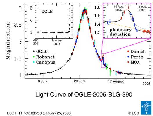
Lensing Potential
n For thin lense we can work using a lensing potential
! 2 ! 2 ! 2
α = 2 ∫ ∇ ⊥Φ dl = 2 ∇ ⊥ ∫ Φ dl = $ %& '
c c #
n Where ∇ ⊥ is a 2D gradient that operates in the lense plane (i.e. only
perpendicular to light travel direction)
n The 2D function j is just the projected gravitational potential
n So the lensing equation can then be written in terms of angular
gradients of a dimensionless 2D lensing potential
DLS
( )
θI − θS = α
DS
≡ ∇θϕ (θ I )
n This shows: (1) any two systems with same projected surface density
have the same lense effect and (2) addition of a mass sheet doesn’t
change the gradient and therefore will not change the lensing effects
of the system
2. Jul 2021 Cosmology and Structure Formation - Mohr - Lecture 7 8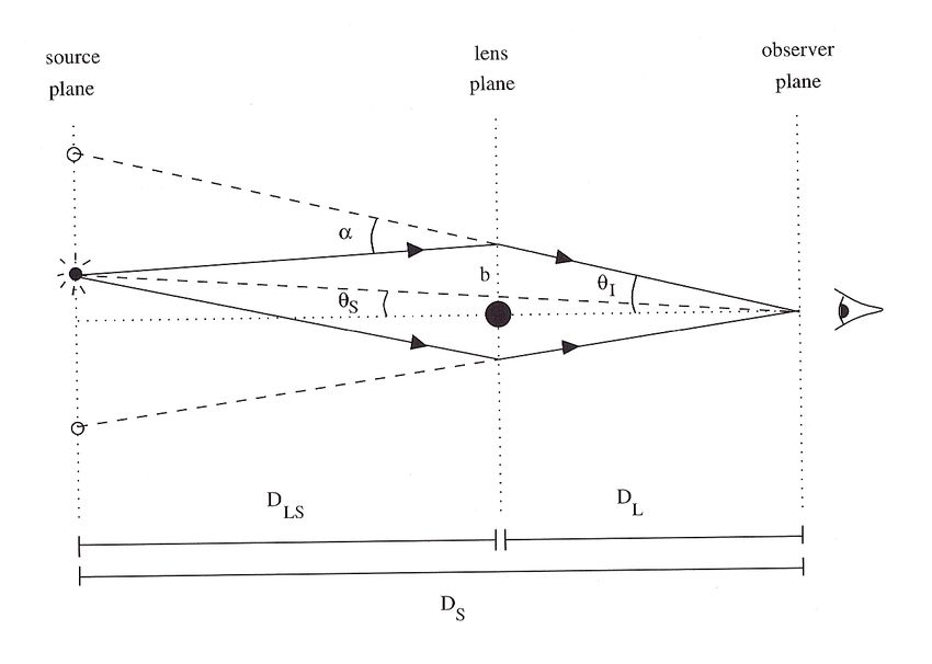
Lensing Potential (cont)
n There is an equivalent to the Poisson equation but in two dimensions
( )
DL DLS 8π G ∑ θI
2
( )
∇ ϕ θI =
θ 2
∑ θI ≡ 2 ( ) ( )
∑ θI = ( )
∫ dl ρ θ I , l
DS c ∑crit
"' +,
where S is the surface density of the thin lens and Σ"#$% = ()* +
- +-.
n In this projected space, force of point mass is 1/r rather than 1/r2 and to get
the potential from the surface mass density we need to convolve with ln(q)
rather than 1/r!
1 2
ϕ (θ ) =
π ∑crit
∫ ∑(θ ") ln θ − θ " d θ "
n This form suggests that departures from thin lense could be treated through
superposition of lensing potentials from many thin lenses
2. Jul 2021 Cosmology and Structure Formation - Mohr - Lecture 7 9Strong Lensing applications
n In strong lensing regime the distortion or magnification is
large and the surface density of the lense is larger than
the critical density Σ"#$%
n Several interesting cosmological applications have been
developed
2. Jul 2021 Cosmology and Structure Formation - Mohr - Lecture 7 10Simple Lens Models: Circularly Symmetric
n Bending angle for a circularly symmetric lense has a
particularly simple form:
4GM(< b)
α=
c 2b
nDistance of closest approach b= DLqI
n M(4GM (< b)
α=
c2b
Bending angles and radial distortions
n Dependence of bending angles on closest approach b
leads to a radial distortion (stretching in case of point
mass) of the background source
n Because the enclosed mass projected within b for an
isothermal sphere scales as b, the bending angle for an
isothermal sphere is the same at all radii. The constant
bending angle means there is no radial distortion
n Generally speaking, radial behavior of arcs provides
constraints on the radial mass distribution of the lense
2. Jul 2021 Cosmology and Structure Formation - Mohr - Lecture 7 12Einstein Ring
n Perfect alignment of observer, lense and source with a
symmetric lense leads to a beautiful Einstein Ring
n In this case qS=0 DS D 4GM
α=
DLS
(θI − θS ) = S θE = 2
DLS cb
b = DLθ E
% 4GM DLS (1 2
θE = ' 2 *
& c DL DS )
n A characteristic value for point source is
€
# M &1 2 # DL DS DLS & −1 2
θ E = % 11.09 ( % ( arcsec
$ 10 M ' $ 1Gpc '
n Galaxy scale masses – arcsec, Galaxy cluster scale masses – arcmin
€
2. Jul 2021 Cosmology and Structure Formation - Mohr - Lecture 7 13Einstein Rings Are Rare But Real!
n An HST image of a blue background galaxy lensed by an LRG. Originally the
system was found in SDSS data
2. Jul 2021 Cosmology and Structure Formation - Mohr - Lecture 7 14Properties of Lenses: Time Delay
n The change in light path caused by lensing has an associated time
delay DL DLS α 2 2Φ
cΔt g + cΔt p = (1+ zL ) − ∫ dl (1+ zL ) 2
DS 2 c
n Where the first term is the geometric time delay that comes from the
fact that the light from the same source travels two different paths to
reach the observer, and the second is the gravitational potential time
€
delay
n The potential time delay comes from clocks ticking more slowly in a
gravitational potential. Note the weak field non-expanding metric:
$ 2Φ ' 2 2 $ 2Φ ' 2
c dτ = &1+ 2 )c dt − &1 − 2 )( dx + dy 2 + dz 2 )
2 2
% c ( % c (
n The two terms are similar in scale, and the potential time delay
requires an accurate model for the lensing potential
2. Jul 2021 Cosmology and Structure Formation - Mohr - Lecture 7 15
€*t, *
417 ^
FIG. 3.ÈThe 1995 A light curves ( Ðlled circles) shifted by the optimal mma
values of the time delay *t and the magnitude o†set *m, superimposed on
the 1996 image B data (open circles). The Ðts are based on the linear
the c
method analysis, but the parameters given by other Ðtting methods are for th
nearly identical. See text for details. Insets show the overlapping regions of corre
A and B light curves assuming the long delay of 540 days (and Ðtting for Ðgur
Time Delay Observed Kundic et al 1997
the magnitude o†set). This delay is clearly excluded by the data.
PRH
In
QSO 0957+561 tistic
of th
n Great effort put into multiply lensed imag
quasar 0957+561. each
data
n There are two relatively bright 4
components that can be imaged
Fo
relatively easily 0957
delay
surem
n Years of monitoring of the light curves of un
conv
of the two brightest components led to diam
a measurement of a time delay. Koc
nate
0957
n Even controversy about value of the amb
Gore
time delay- values ranged from 400 to Shap
550 days obse
free
. tanc
the l
the t
(Cha
Pacz
FIG. 4.ÈOptimal PRH reconstruction of the shifted and combined A
( Ðlled circles) and B (open circles) light curves of 0957]561. The shaded
tion
region (““ snake ÏÏ) corresponds to the 1 p conÐdence interval of the recon- Ðve-
2. Jul 2021 Cosmology and Structure Formation - Mohr
struction. The error -bars
Lecture
are the 7
photometric 1 p measurement errors.16 andHubble Parameter Constraints
n Modeling of multiply lensed quasar 0957+561.
n Interpretation is quite difficult, because the geometric and the potential terms in the
time delay are comparable, and to calculate the potential term one must know the
gravitational potential along the line of sight through the lens.
n Grogan and Narayan 1996 put a lot of effort into building a model for the lense
# σv & 2 # Δt & −1
H o = ( 79 ± 7km/s/Mpc)% (% (
$ 300km/s ' $1yr '
n Follow-on observational work by Kundic et al (1997) on the lense velocity
dispersion and time delay led to the final result
€ H o = 64 ±13km/s/Mpc
n Constraints from this approach are broadly consistent with Hubble
parameter constraints from other methods, but the results suffer from
significant lens modeling uncertainties
2. Jul 2021 Cosmology and Structure Formation - Mohr - Lecture 7 17Renewed effort focused on this problem
n Large numbers of new strong lensing systems are discovered with
ever improving surveys (SDSS, PS, DES, Euclid, Rubin)
n Time domain information obtained as part of data acquisition strategy
in Rubin (fully sky imaged every ~3 days)
n H0 “tension” makes this work very relevant
n Some recent references for further information
n “… a 2.4% measurement of H0 from lensed quasars…”
https://ui.adsabs.harvard.edu/abs/2020MNRAS.498.1420W/abstract
n “Measuring angular diameter distances of strong gravitational lenses”
https://ui.adsabs.harvard.edu/abs/2015JCAP...11..033J/abstract
2. Jul 2021 Cosmology and Structure Formation - Mohr - Lecture 7 18Microlensing to study compact objects
n Significant amplification can result from even a stellar mass object
passing sufficiently close to the line of sight to a distant star
n The Einstein radius of the lens is so small that what is observed is an
amplification of the light from the background star
n Powerful technique to probe the compact object population of our own
galaxy (whether baryonic or not)
2. Jul 2021 Cosmology and Structure Formation - Mohr - Lecture 7 19Microlensing Results
n Optical depth for lensing is very small, but this can be overcome by
monitoring large populations of stars
σ v2 DL DLS
τ = 2π 2 ≈ 5x10 −7 to LMC
c rDS
n Two leading teams – MACHO and OGLE- monitored large star fields for
years €
and found microlensing events
n For each real event they found 100’s of variable stars
n Color-independence of gravitational lensing allows the microlensing to be separated
out from normal stellar variability
n Bottom line is that the Milky Way halo mass is composed of about ~ 10%
compact objects, and these compact objects have a characteristic mass
of ~0.6 Mo, which is the typical mass of a white dwarf.
2. Jul 2021 Cosmology and Structure Formation - Mohr - Lecture 7 20Now used to study planets
n Interesting the microlensing can be impacted by the presence of
multiple compact objects bound together– planetary systems
see, e.g., http://www.planetary.org
2. Jul 2021 Cosmology and Structure Formation - Mohr - Lecture 7 21Weak lensing and applications
n Gravitational lensing is ubiquitous in the Universe but typically the
distortions and magnification effects are quite small à the weak
lensing regime where the surface density of the lense is small
compared to the critical density
n Weak lensing of background galaxies by foreground lenses (galaxies,
clusters or galaxies and large scale structure) is regularly employed
now to measure halo masses or to characterize the power spectrum
of density fluctuations
n Weak lensing of the CMB itself has been employed recently in an
attempt to study halo masses
2. Jul 2021 Cosmology and Structure Formation - Mohr - Lecture 7 22Lensing Potential
n For thin lense we can work using a lensing potential
! 2 ! 2 !
α = 2 ∫ ∇ ⊥Φ dl = 2 ∇ ⊥ ∫ Φ dl
c c
n Where ∇ ⊥ is a 2D gradient that operates in the lense plane (i.e. only
perpendicular to light travel direction)
n The 2D function j is just the projected gravitational potential
n So the lensing equation can then be written in terms of angular
gradients of a dimensionless 2D lensing potential
DLS
( )
θI − θS = α
DS
≡ ∇θϕ (θ I )
n This shows: (1) any two systems with same projected surface density
have the same lense effect and (2) addition of a mass sheet doesn’t
change the gradient and therefore will not change the lensing effects
of the system
2. Jul 2021 Cosmology and Structure Formation - Mohr - Lecture 7 23Properties of Thin Lenses: Shear and Convergence
n Differentiating the lense equation (noting that angles are actually 2D vectors), we can
express the components of the Jacobian as:
! ∂θ $ ∂ 2
ϕ
()
A θ = # I & = δij +
" ∂θ S %ij ∂θ i∂θ j
(θ I − θ S ) = ∇θϕ (θ I )
n This formulation is useful for describing small distortions of shape and amplitude in the
weak (linear) regime.
n It is common to see the Jacobian written as:
" 1+ γ1 − κ −γ 2 %
()
A θ =$
$# −γ 2 1− γ1 − κ
'
'&
where g is the shear and k is the convergence
n With respect to the underlying partial derivatives the definitions are
1 " ∂2ϕ ∂2ϕ % 1 " ∂2ϕ ∂2ϕ % ∂2ϕ
κ= $ + ', γ1 = $ − ', γ 2 =
2 # ∂θ1∂θ1 ∂θ 2∂θ 2 & 2 # ∂θ1∂θ1 ∂θ 2∂θ 2 & ∂θ1∂θ 2
2. Jul 2021 Cosmology and Structure Formation - Mohr - Lecture 7 24Properties of Thin Lenses: Reduced Shear
n It is common to see the Jacobian written as:
" 1+ γ1 − κ −γ 2 % " 1+ g −g %
()
Aθ = $
$# −γ 2 1− γ1 − κ
' = (1− κ )$
'&
1 2
$# −g2 1− g1
'
'&
where g is the reduced shear
( )
γ θ
( ) 1− κ θ
gθ =
()
n The shear and reduced shear have two components and can be written as complex numbers
g = g1 + ig2 = g e 2iϕ
n The amplification of a source is then expressed as
! δθ I2 $ 1 1
# 2& = = 2
δθ
" S% det A ( ) − γ12 − γ 22
1− κ
2. Jul 2021 Cosmology and Structure Formation - Mohr - Lecture 7 25Properties of Thin Lenses: Critical Surface Density
n Given earlier 2D Poisson equation for the lensing potential we can relate the
convergence k to the lense surface density
DL DLS 8π G ∑
∇θ2ϕ = ∑ ≡ 2
DS c2 ∑crit
2 ∂2ϕ ∂2ϕ
∇ ϕ = 2 + 2 = tr [ A ]
θ
∂ θx ∂ θy
n The convergence is then related to the ratio of the surface density to the critical surface
density, where the critical density is that corresponding to a bending angle that would
refocus the light
∑
κ=
∑crit
2. Jul 2021 Cosmology and Structure Formation - Mohr - Lecture 7 26Mass Measurements and Mapping
n Gravitational lensing in the weak regime is now used routinely to map the
distribution of matter in clusters and has also been used to map the matter
fluctuation power spectrum and to constrain the halos of ensembles of
galaxies
n In this regime we don’t get the multiple lensing seen in strong lensing– rather,
we get only the weak distortions of the shapes of galaxies caused by the
lensing matter between the observer and the source
n Consider Jacobian A of transformation from source plane I(s)(b) to the
observer or image plane I(q). (Remember: surface brightness is conserved)
! ∂β $ ∂ 2ϕ
i
I(θ ) = I (s) (β (θ )) ## && = Aij = δij +
" ∂θ j % ∂θ i∂θ j
2. Jul 2021 Cosmology and Structure Formation - Mohr - Lecture 7 27Shear and Convergence
n The Jacobian matrix A describes a
linearized lens mapping from source β − βo = A (θ o ) ⋅ (θ − θ o )
plane Is(b) to image/observer plane
I(q) I(θ ) = I (s) #$βo + A(θ o )⋅ (θ − θ o )%&
n k is the convergence " 1− g −g %
1 2
n g is the reduced shear A (θ ) = (1− κ ) $ '
g is the gravitational shear
$ −g2 1+ g1 '
n
# &
n The shear and the reduced shear
are both polar quantities (like γ (θ )
vectors) that can be conveniently g (θ ) =
"#1− κ (θ )$%
written as complex numbers
n Factor of two in the phase reflects the γ = γ1 + iγ 2 = γ e 2iφ
symmetry of ellipse under 180o rotation,
and this differentiates shear from vector g = g1 + ig2 = g e 2iφ
(See discussion Section 2.3, Schneider)
2. Jul 2021 Cosmology and Structure Formation - Mohr - Lecture 7 28its image is an ellipse, with semi-axes
R R R R
= ; =
1 − κ − |γ| (1 − κ)(1 − |g|) 1 − κ + |γ| (1 − κ)(1 + |g|)
and the major axis encloses an angle ϕ with the positive θ1 -axis. Hence,
if sources with circular isophotes could be identified, the measured image
Weak Lensing Distorts Intrinsic Light Distribution
ellipticities would immediately yield the value of the reduced shear, through
the axis ratio
1 − b/a b 1 − |g|
|g| = ⇔
n Because these are small distortions,
1 + b/a the
a Jacobian
=
1 + |g| describing the
transformation from theof source
and the orientation the major to
axisthe image
ϕ. In planeitiswas
these relations close to the unit
assumed
matrix that b ≤ a, and |g| < 1. We shall discuss the case |g| > 1 later.
convergence and
shear
S D
A−1 ϕ
β2 θ2
β1 θ1
s
! convergence only
O
!
Fig. 1. A circular source, shown at the left, is mapped by the inverse Jacobian A−1
onto an ellipse. In the absence of shear, the resulting image is a circle with modified
radius, depending on κ. Shear causes an axis ratio different from unity, and the
orientation of the resulting ellipse depends on the phase of the shear (source: M.
Bradac)
2. Jul 2021 Cosmology and Structure Formation - Mohr - Lecture 7 29
However, faint galaxies are not intrinsically round, so that the observed
image ellipticity is a combination of intrinsic ellipticity and shear. The strat-Induced Ellipticity of Source Galaxies
n A circular source of radius R would
have semi-major (semi-minor) axis a R R
a= =
(b) depending on convergence k and 1− κ − γ (1− κ ) (1− g )
reduced shear g
R R
b= =
1− κ + γ (1− κ ) (1+ g )
n Thus, for a circular source the
observed axial ratio r=b/a delivers a 1− b b 1− g
g= a ⇔ =
measure of the reduced shear
1+ b a 1+ g
a
2. Jul 2021 Cosmology and Structure Formation - Mohr - Lecture 7 30Measuring Source Ellipticities
n Source ellipticities are related to the
second moment tensor Q of the light
First Moment Vector
distribution. The center of mass of the
object is the first moment. 2
∫ θ I '(θ )W (θ )θ
d
θ= 2
∫ θ I '(θ )W (θ )
d
n Radial weighting functions W(q) are
typically adopted to optimize the signal to
Second Moment Tensor
noise
∫ d θ I '(θ )W (θ ) (θ − θ ) (θ
2
i i j −θ j )
Qij = 2
n This second moment tensor Q of the light ∫ d θ I '(θ )W (θ )
distribution can then be diagonalized to
determine axial ratio and orientation. The
trace of Q gives the size of the object.
2. Jul 2021 Cosmology and Structure Formation - Mohr - Lecture 7 31Complex Ellipticities c and e
n Schneider introduces two
complex ellipticities c and e as
well
Q11 − Q22 + 2iQ12
χ≡
Q11 + Q22
Q11 − Q22 + 2iQ12
ε≡ 1 c2
Q11 + Q22 + 2 (Q11Q22 − Q 2
) 2
12
n Both share same phase, but
amplitudes differ and are useful
in different contexts
1− r 2 1− r
χ = and ε =
1+ r 2 1+ r c1
where r is the axial ratio
2. Jul 2021 Cosmology and Structure Formation - Mohr - Lecture 7 32Estimating Intrinsic Source Ellipticities
n In the weak lensing regime it is
possible to directly estimate the (s) T
pre-lensing moments of the light
Q = AQA
distribution of sources, given the
model of the lens (s) χ − 2g + g 2 χ *
χ = 2
1+ g − 2Re ( g χ * )
n Recovering the source plane 2nd
moment Q(s) requires a simple
matrix manipulation # ε−g
% if g ≤ 1
(s) % 1− g*ε
n The source plane complex ε =$
% 1− gε *
ellipticities c(s) and e(s) can be %
if g > 1
written in terms of the observed & ε * − g*
ellipticities and the reduced shear
2. Jul 2021 Cosmology and Structure Formation - Mohr - Lecture 7 33sin(2ϕ), or simply, the complex shear gets multiplied by
this transformation behavior of the shear traces back to
as the traceless part of the Jacobi matrix A. This trans
the same as that of the linear polarization; the shear i
analogy with vectors, it is often useful to consider the
a rotated reference frame, that is, to measure them w
Tangential and Radial Component of Shear tion; for example, the arcs in clusters are tangentially
ellipticity is oriented tangent to the radius vector in th
n For circularly symmetric
α = 0◦
projected mass distributions, $t = 0.3
$× = 0.0
α = 45◦
$t = 0.0
the shear is tangentially $× = 0.3
oriented with respect to the Fig. 3. Ill
tial and c
direction toward the lense φ α = 90◦
shear, for
$t = −0.3 !2 = 0, an
center. O $× = 0.0 tions φ wi
point (sou
n For this reason it’s typical in
cluster studies to adopt If φ specifies a direction, one−2i
defines the tangential
“tangential” and “cross” γ = − Re "#γ e $%φ
of the shear relative to this direction as
t
components of the shear !
γt = −Re γ e−2iφ
"
, γ× = −Im γ e
!
γ
For example, = − Im "
x in case of a #γ e −2iφ $
%
circularly-symmetric matter d
at any point will be oriented tangent to the directio
2. Jul 2021 Cosmology and Structure Formation - Mohr - Lecture 7 34Applications: Weak lensing shear
n We have now introduced the the shear and its connections to the observed
ellipticity and orientation of galaxies
n The shear distortion is a stretching of the light distribution of sources, and that
distortion is directly related to the derivatives of the 2D lensing potential
! ∂β $ ∂ 2
ϕ
## i && = Aij = δij +
" ∂θ j % ∂θ i∂θ j
n For an isothermal sphere mass distribution this shear leads to tangential
stretching. The observed tangential shear field as a function of distance from
the center of the mass distribution then constrains the projected mass profile
of the isothermal sphere, which provides 3D density model (geometry
dependent)
n For more general mass distributions it remains possible to measure the
properties using the observed shear field. We will discuss more in a bit.
2. Jul 2021 Cosmology and Structure Formation - Mohr - Lecture 7 35Applications: Weak lensing magnification
n The Jacobian encodes the change in the area of the source, and given the
surface brightness is conserved in lensing (Liouville’s theorem) the
determinant of A provides the amplification or magnification µ
1 1
µ= = 2
≈ 1+ 2κ
det [ A ] (1− κ ) − γ 2
n Amplification tends to be weak and is difficult to detect because there is a
distribution of brightnesses of galaxies
n The increased number of galaxies due to small amplification is compensated by the 1/A
decrease in the galaxy surface density due to the same magnification
n The net effect depends on how steeply the number of galaxies increases as a function of
magnitude
n Recently, there is a flowering of interest in this technique as a cross-check
of the shear and as a way of increasing the signal to noise of the lensing
constraints (i.e. on cluster masses).
n See Umetsu et al 2011 “Cluster mass profiles from a bayesian analysis of weak lensing
distortion and magnification measurements: applications to SUBARU data”
2. Jul 2021 Cosmology and Structure Formation - Mohr - Lecture 7 36Magnification in SPT Selected Clusters
Chiu+2016
n We studied this in sample of 19Magnification
SPT selected clusters. The signal in our data
bias of background galaxies 7
was weak but detectable (3.3s), corresponding to ~25% accurate masses.
'(()
⃗ =
!($) and
')*+,
.2 6
Σ./01 = and
345 789
89;
:=
8;
Figure 3. Illustration of the colour-colour background selection in the case of SPT-CL J0234 5831 (z = 0.42) with magnitude cuts 20.0 6 g 6 23.5. On
the left is the g r versus r i colour-colour diagram showing the observed galaxy density distribution (gray scale), the passively evolving cluster galaxy
population (green), the z ⇡ 0.9 background (orange) and the z ⇡ 1.8 background (blue). The corresponding normalized redshift probability distribution P(z)
estimated from CFHTLS-DEEP for each population is shown on the right. The green dashed line marks the cluster redshift.
at zl = 0.42, where lected galaxies to the redshift information taken from the reference
2. Jul 2021 Z
hb il = Pref (z)µ(M500 , zl , z)2.5s 1 b (z)dz
Cosmology
(15)
and
field. Structure
Specifically, Formation
we use - Mohr by- Lecture
the method developed Gruen et al.7 37
(2014), in which they estimated the fraction of the cluster galaxies
contaminating the background population by decomposing the ob-
and Pref (z) is the redshift distribution of the reference field where served distribution of the lensing efficiency, P(b ), into the knownMagnification in SPT Selected Clusters
Chiu+2016
n We studied this in sample of 19 SPT selected clusters. The signal in our data
12 Chiu et al.
was weak but detectable (3.3s), corresponding to ~25% accurate masses.
Figure 7. The stacked profiles for the low- and high-z background populations with the best-fit models from different scenarios. The panels contain the fit to
the low-z background alone (left), the fit to the high-z population (middle), and the fit to the combined population (right). In all three panels the orange circles
(blue squares) define the stacked profile of the low-z (high-z) population, the best-fit model is defined with solid lines and the predicted profile for the other
population appears as a dot-dashed line. There is slight (⇡ 1.82s ) tension between the low- and high-z populations, whereas the joint fit (right panel) is in
good agreement with both populations.
Table 3. Magnification analysis mass constraints, cross checks and detection significance. Column 1: background populations used in the fit. Column 2:
Cosmology
2. Jul 2021best-fit h. Column 3–5: 1, 2, and 3 s confidence andh. Structure
level of the best-fit Formation
Column 6: reduced - Mohr
Cstat of the fit (degree - Lecture
of freedom: 7 21 for the low-z, the
10, 10 and 38
high-z and the combined backgrounds, respectively). Columns 7–8: p-value that the best-fit model in Column 2 rejects the best-fit model in these columns.
Column 9: detection significance over a model with h = 0.WL Shear Observational Considerations (1)
n The weak lensing shear is small (~few % at the largest) whereas the intrinsic
ellipticity distribution of galaxies has an rms variation at the level of 25%
n Large numbers of sources must be combined across a region where the
shear is coherent to enable a statistically significant constraint
2
2 2 σ gal
γ WL = 1
N ∑ γi 1
σ γWL= ( N−1) ∑ (γ i − γ WL ) ≈
N gal
i=1,N i=1,N
n Thus, to reach a 1% uncertainty on the shear measurement one has to
combine shear measurements of ~600 galaxies
n Characteristic number densities of suitable galaxies for deep optical imaging
from the ground/space range from 10 galaxies/arcmin2 to 60 galaxies/arcmin2,
setting a minimum required survey area for the weak lensing measurement
2. Jul 2021 Cosmology and Structure Formation - Mohr - Lecture 7 39WL Shear Observational Considerations (2)
n Averaging down the shear measurements of individual galaxies to
obtain the underlying weak lensing shear assumes there are no
systematic biases in the individual shear measurements
n Observationally, this means the distortions introduced by the imager must be
removed with high accuracy
n In addition, one must be concerned about whether there are any
intrinsic alignments among galaxies
n These can result from tidal interactions arising from the surrounding large scale
structure that is common to populations of neighboring galaxies
2. Jul 2021 Cosmology and Structure Formation - Mohr - Lecture 7 40Imaging Distortions: Non-Lensing Shear
n Distortions can be quite large in Geometric Distortion ESO WFI
typical wide field imagers
n Wide Field Imager (WFI) images
show resulting shifts in object -11.4
positions due to optical
distortions.
n Variation of positional shifts with -11.6
focal plane position leads to
stretching or compression of the
light distribution in the image
plane (i.e. shear!)
-11.8
n Whisker diagrams show orientation
and ellipticity of stars within an
image. This is a direct measure of 174.8 174.6 174.4 174.2
the instrumental distortion. Ra
2. Jul 2021 Cosmology and Structure Formation - Mohr - Lecture 7 41Mapping Imager Distortions
n Distortions can be mapped using BTC Whisker Plot
the shapes of stars, which are
unresolved sources (unaffected
by weak lensing)
n Big Throughput Camera (BTC)
Whisker Plot shows the shear
distortion that is mapped by the 1% ellipticity
stars within the field
n Corrections can be calculated from
the stars and applied to all objects
(stars and galaxies), revealing the
intrinsic shear field
2. Jul 2021 Cosmology and Structure Formation - Mohr - Lecture 7 42Mapping Imager Distortions
n Distortions can be mapped using Whiskers After Distortion Corrections
the shapes of stars, which are
unresolved sources (unaffected
by weak lensing)
n Big Throughput Camera (BTC)
Whisker Plot shows the shear
distortion that is mapped by the 1% ellipticity
stars within the field
n Corrections can be calculated from
the stars and applied to all objects
(stars and galaxies), revealing the
intrinsic shear field
2. Jul 2021 Cosmology and Structure Formation - Mohr - Lecture 7 43Correcting Imager Distortions
n The density of stars on the sky used to map
the shear distortions places a fundamental -11.4
limit on how well these distortions can be
measured (and corrected)
n ~1 star/arcmin2 is characteristic number (depends -11.6
on depth, cannot use saturated stars)
n Distortions are typically not smoothly varying
Distortions change from exposure to exposure due
-11.8
n
to telescope tracking and atmosphere changes 174.8 174.6 174.4 174.2
Ra
n High precision weak lensing seeks to control imager distortions to ~0.01%
n Requires a camera that is very stable over time, so that PSF information about the
imager distortions can be combined from multiple observations
n Go to space: diffraction limited imaging, constant environmental conditions
n EUCLID mission designed with lensing as goal! See http://arxiv.org/abs/1110.3193
2. Jul 2021 Cosmology and Structure Formation - Mohr - Lecture 7 44WL Shear Sensitivity and Meta-Calibration
n A tiny shear !"#$% is introduced into
n Galaxies have intrinsic shear (are the image of each object along
elliptical with random orientation) orthogonal directions (shear is
polar quantity), and then a shear
n Image noise and PSF asymmetries measurement !&%'( is extracted.
add additional challenges )*
The shear sensitivity +,-. is then
)*/01,
extracted, providing an orientation
n Direct image simulations allow one dependent shear weighting for
to extract the sensitivity of each each measurement
galaxy to a putative underlying
weak lensing shear signature
n This approach is now the standard
within Dark Energy Survey and is
n METACALIBRATION (Huff & planned as the standard within
Mandelbaum, Sheldon & Huff Rubin (additional challenges come
2017) is one such method with undersampled images like
those from Euclid)
2. Jul 2021 Cosmology and Structure Formation - Mohr - Lecture 7 45Photometric redshifts are crucial
n Weak lensing observables (shear n Within weak lensing context one is
and magnification) are sensitive to using distortions in many faint
the projected surface density over background galaxies to infer the
foreground mass distribution. The is
the critical density
therefore an effective Σ./01 for the
'(() ensemble
⃗ =
e.g., !($)
')*+,
n Critical density Σ./01 captures the n It is impractical to measure
geometry of the source-lense spectroscopic redshifts for every
system source– so this work relies on
photometric redshift estimates
.2 6 89;
Σ./01 = and : =
345 789 8;
n Broad band photometry (e.g., grizY) is
used to estimate redshift of each
n Redshifts are the observable, and galaxy. Measurement uncertainty must
distance-redshift relation is be accounted for in calculating Σ./01
cosmologically sensitive and biases must be minimized
2. Jul 2021 Cosmology and Structure Formation - Mohr - Lecture 7 46WL Shear Studies of Galaxy Clusters
n Weak lensing masses of galaxy clusters are crucially
important for cluster cosmological studies
n Weak lensing mass constraints do not depend on the
dynamical state of the cluster; weak lensing works well
even for merging systems
n Strong lensing is also valuable, but the strong lensing
region corresponds to the innermost regions in galaxy
clusters, whereas for cosmology it is important to
characterize the cluster masses out to larger radius
2. Jul 2021 Cosmology and Structure Formation - Mohr - Lecture 7 47ß ~0.6 Mpc à
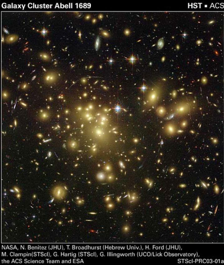
Abell 1689
n HST ACS images reveal
the cluster galaxies
(yellow) and many
tangentially distorted strong
lensing arcs
n Mass reconstruction of the
central regions is possible
using these many arcs
n See Tyson et al 1998
“Detailed Mass Map of CL
0024+1654 from Strong
Lensing”
n Weak lensing benefits from
a much larger field
2. Jul 2021 Cosmology and Structure Formation - Mohr - Lecture 7 48ß ~6 Mpc à
Abell 1689
Weak Lensing
n Mass extraction:
WFI Images
*
Shear Field
*
2D Lensing Potential
*
Surface Density Distribution
*
Density Distribution
*
Cluster Mass Measurement
n Top: contour plot of mass
n Bottom: profile of reduced shear
2. Jul 2021 Cosmology and Structure Formation - Mohr - Lecture 7 49The Shear Mass of SPT-CL J2022-6323
n The tangential and cross shear profiles are shown below (left) from
High et al 2012 Σ < $ − Σ($)
!" ($) =
Σ*+,"
n The inferred aperture mass is plotted (right) as a function of projected
Fig. 10.— SZ, optical, and data for SPT-CL J2022-6323. See Section A for a description.
radius of the cluster. The cyan region corresponds to the 68%
confidence region
n This mass is compared Mass model
to the cluster mass
estimated from an X-ray
method (open circle with
error bar); in this case
mass estimates agree
well
Cross-shear profile consistent with zero
Fig. 11.— Shear and aperture mass profiles of SPT-CL J2022-6323. See Section A for a description.
2. Jul 2021 Cosmology and Structure Formation - Mohr - Lecture 7 50Challenges to Cluster WL Shear Studies
n Clusters are the most massive collapsed objects, and this makes them among
the best targets for weak lensing mass measurements
n However, there are several challenges in extracting cluster weak lensing masses
n Mass sheet degeneracy- any component of the cluster mass that produces an approximately flat
projected mass distribution over the angular scale of the imaging will be lost in a shear analysis-
drives one to larger fields around clusters
n Source redshift distribution- masses depend on ratios of distances to the lense and sources. The
cluster redshift is straightforward, but the source redshifts are a challenge.
n Contamination of source sample- cluster galaxies or foreground galaxies are not lensed by the
cluster, and any residual contamination of the source shear population will bias the cluster mass low
n Large scale structure- all mass components along the line of sight contribute to the observed shear.
This large scale structure varies along each line of sight adding an astrophysical noise source to the
mass measurement (depends on angular scale of the observation- characteristically ~10% for
massive cluster, but 25% to 50% for low mass clusters)
n Mis-centering: to extract the mass constraints one fits the projected profile. But the shear profile
depends on the choice of cluster center
2. Jul 2021 Cosmology and Structure Formation - Mohr - Lecture 7 51Stacking of Clusters to Reduce Noise
n The large scale structure noise varies
from cluster to cluster. The noise in
the measured shear field has both
statistical and systematic
components.
n Combining observations from multiple
clusters provides a way of reducing
the random noise components
n In this approach one must carefully
characterize systematic sources of
noise, because they quickly start to Stacked shear profile from Umetsu et al 2011 “A
dominate as one stacks information Precise Cluster Mass Profile Averaged from the
from large numbers of clusters Highest-quality Lensing Data”
NFW Concentration c=7.68+/-0.4
2. Jul 2021 Cosmology and Structure Formation - Mohr - Lecture 7 52Cluster Weak Lensing Summary
n Cluster mass measurements using weak lensing shear are now
becoming routine, but WL magnification needs further development
n Coordinated observational and theoretical/mock observational
programs are the most powerful
n Can characterize scale of shear measurement systematics
n Can test the impact of large scale structure and correct for it
n Can probe the required accuracies for source galaxy photo-z’s
n In principle these masses can be accurate at better than the 5% level
n This is a major focus of our SPT/DES/eROSITA/Rubin/Euclid program
here at LMU
2. Jul 2021 Cosmology and Structure Formation - Mohr - Lecture 7 53Cosmic Shear:
Shear Induced by the Large Scale Structure
n Cosmic shear measures the mass distribution over the
range of redshifts where one has sources
n This mass distribution need not be in the linear regime- collapsed
objects are measured as well
n With photo-z’s of the source galaxies, it is possible to
carry out cosmic shear tomography, where the mass
distribution is measured as a function of redshift
n This provides a powerful constraint on the growth of structure
2. Jul 2021 Cosmology and Structure Formation - Mohr - Lecture 7 54WL Shear Tomography
3
Given photometric redshifts for the
[ ni dz/dD ](D)
n (a) Galaxy Distribution
source galaxies, it is possible to 2
extract information about the redshift 1 1 2
distribution of the underlying structure
0.3 (b) Lensing Efficiency
n Simply stated, a source galaxy is impacted
gi(D)
only by the matter distribution between it 0.2
2
and the observer 0.1
n Examining the shear power spectrum as a 1
function of the redshifts of the source 0 0.5 1 1.5 2.0
D
galaxies then allows one infer the redshift
distribution of the clustered matter Hu 1999 “Power Spectrum Tomography
n This allows cosmic shear to be used with Weak Lensing” discusses how even
by dividing the source galaxies into crude
to directly measure the growth rate of redshift bins one can recover information
cosmic structures with time. and the growth of structure, allowing
much more sensitive cosmological
studies
2. Jul 2021 Cosmology and Structure Formation - Mohr - Lecture 7 55Lensing Potential
n For thin lense we can work using a lensing potential
! 2 ! 2 !
α = 2 ∫ ∇ ⊥Φ dl = 2 ∇ ⊥ ∫ Φ dl
c c
n Where ∇ ⊥ is a 2D gradient that operates in the lense plane (i.e. only
perpendicular to light travel direction)
n The 2D function j is just the projected gravitational potential
n So the lensing equation can then be written in terms of angular
gradients of a dimensionless 2D lensing potential
DLS
( )
θI − θS = α
DS
≡ ∇θϕ (θ I )
n This shows: (1) any two systems with same projected surface density
have the same lense effect and (2) addition of a mass sheet doesn’t
change the gradient and therefore will not change the lensing effects
of the system
2. Jul 2021 Cosmology and Structure Formation - Mohr - Lecture 7 56Properties of Thin Lenses: Shear and Convergence
n Differentiating the lense equation (noting that angles are actually 2D vectors), we can
express the components of the Jacobian as:
! ∂θ $ ∂ 2
ϕ
()
A θ = # I & = δij +
" ∂θ S %ij ∂θ i∂θ j
(θ I − θ S ) = ∇θϕ (θ I )
n This formulation is useful for describing small distortions of shape and amplitude in the
weak (linear) regime.
n It is common to see the Jacobian written as:
" 1+ γ1 − κ −γ 2 %
()
A θ =$
$# −γ 2 1− γ1 − κ
'
'&
where g is the shear and k is the convergence
n With respect to the underlying partial derivatives the definitions are
1 " ∂2ϕ ∂2ϕ % 1 " ∂2ϕ ∂2ϕ % ∂2ϕ
κ= $ + ', γ1 = $ − ', γ 2 =
2 # ∂θ1∂θ1 ∂θ 2∂θ 2 & 2 # ∂θ1∂θ1 ∂θ 2∂θ 2 & ∂θ1∂θ 2
2. Jul 2021 Cosmology and Structure Formation - Mohr - Lecture 7 57Lensing Potential (2D Poisson Eqn.)
n There is an equivalent to the Poisson equation but in two dimensions
( )
DL DLS 8π G ∑ θI
2
( )
∇θϕ θ I = 2 ( )
∑ θI ≡ 2 ∑ θ I = ∫ dl ρ θ I , l( ) ( )
DS c ∑crit
where S is the surface density of the thin lens
n This form suggests that departures from thin lense could be treated
through superposition of lensing potentials from many thin lenses
2. Jul 2021 Cosmology and Structure Formation - Mohr - Lecture 7 58Weak Gravitational Lensing 79
Cosmic Shear Wm=1
Simulations
n Projected mass
distributions for two
cosmological models
(left) and the
corresponding shear
fields (right)
n Differences in large Wm=0.3
scale structure between
cosmological models
can be measured using
cosmic shear studies
n Tomography allows the
projected mass
distribution to be
measured as a function
of redshift
Fig. 26. Projected mass distribution of the large-scale structure (left), and the
2. Jul 2021 Cosmology and Structure
corresponding Formation
shear field (right),- where
Mohr - the
Lecture 7 and orientation of the sticks
length 59
indicate the magnitude and direction of the local shear. The top panels correspond
to an Einstein–de Sitter model of the Universe, whereas the bottom panels are forWL Shear Correlation Function
n Shear dispersion is the
variance in the mean shear 2 1
measured within spherical γ (θ ) =
2π
∫ dl lP (l ) W (lθ )
κ TH
apertures of radius q
WTH is the top hat filter function
n The underlying sensitivity is
to the power spectrum of the
Pk(l) is the power spectrum of the
projected density surface mass density
perturbations Pk(l)
2
γˆ (l ) γˆ* (l ') = ( 2π ) δ (l − l ') Pκ (l )
n The power spectrum of the with tomography one measures P(l) as f(z)
shear is the same as Pk(l) è P(k,z)
2. Jul 2021 Cosmology and Structure Formation - Mohr - Lecture 7 60Convergence Power Spectrum
n The convergence power spectrum is related to the 3D power
spectrum Pd through a line integral that accounts for the lensing
efficiency W(c) of the matter at particular distance fK(c) given the
redshift distribution of the background galaxies
- 0123
9 ) *+ )
ℓ
!" ℓ = Ω( . 45 6 5 !7 8= ,5
4 , / 9: 5
with tomography one measures P(l) as f(z)
è P(k,z)
2. Jul 2021 Cosmology and Structure Formation - Mohr - Lecture 7 61114 P. Schneider
Sitter model can already be excluded from these early results, but the other
three models displayed are equally valid approximations to the data.
Cosmic Shear Results
n Shear dispersion as a
function of circular
aperture radius is
shown from 5
different experiments
(circa 2000)
n All provide highly
significant detections
of cosmic shear and
all are in good
agreement
Fig. 39. Shear dispersion as a function of equivalent circular aperture radius as
2. Jul 2021 Cosmology
obtainedand Structure
from Formation
the first - Mohr - Lecture
five measurements 7
of cosmic 62 et al.
shear (MvWM+: Maoli
2001; vWME+: van Waerbeke et al. 2000; KWL: Kaiser, Wilson & Luppino 2000;
BRE: Bacon, Refregier & Ellis 2000; WTK: Wittman et al. 2000). The data pointsFig. 14. Constraints on Ωm and w from our 3D weak lensing of the employed residual shear correction (Sect. 4), which we es-
analysis of COSMOS for a flat wCDM cosmology, assuming a timate to be 1% in σ8 . From the joint analysis with WMAP-5 we
prior w ∈ [−2, 0]. The contours indicate the 68.3% and 95.4% find
credibility regions, where we have marginalized over the param-
eters which are not shown. The non-linear blue-scale indicates Ωm = 0.266+0.025+0.057
−0.023−0.042
the highest density region of the posterior.
σ8 = 0.802+0.028+0.055
−0.029−0.060 (68.3%/95.4% conf., MS-calib.),
Cosmic Shear Correlation Function
sive probability ratios for wCDM versus ΛCDM of 52 : 48
(w ∈ [−2, 0]) and 45 : 55 (w ∈ [−3.5, 0.5]), confirming that the
which reduces the size of WMAP-only 1σ (2σ) error-bars on
average by 21% (27%). We plot the joint and individual con-
data are fully consistent with ΛCDM.
n Recent results show promise, straints in Fig. 15, illustrating the perfect agreement of the two
as of 2010,
independent constraints
cosmological probes. were very weak
demonstrating thatthecosmic
6.4. Model recalibration with shear and
Millennium Simulation
joint constraints with WMAP-5
using modern datasets together with
Heitmann et al. (2008) and Hilbert et al. (2009) found that the 1.4
CMB anisotropy
Smith et al. constraints
(2003) fitting functions provide
slightly underestimate non-a
Lensing+WMAP
Lensing
linear corrections to the power spectrum. To test whether this
clear indication
has a significant influenceofoncosmic
our results,acceleration
we performed a 1.2 WMAP
3D cosmological parameter estimation using the mean data
vector of the 288 COSMOS-like ray-tracing realisations from 1.0
the Millennium Simulation. Here we modify the strong pri-
So now four different methods have
σ8
n ors given in Sect. 6.1 to match the input values of the simula-
tion (Ωm = 0.25, σ8 = 0.9, ns = 1, h = 0.73, Ωb = 0.045), and 0.8
shown independently that the energy
11
find σ8 = 0.947 ± 0.006 for Ωm = 0.25. This confirms the re-
density of the universe is dominated
sult of Heitmann et al. (2008) and Hilbert et al. (2009), indi-
cating that models based on Smith et al. (2003) slightly under-
0.6
by dark energy
estimate the shear signal, hence a larger σ8 is required to fit
the data. Here we use actual reduced shear estimates from the 0.4
Sne distances (‘99), Galaxy Clusters (‘03), Galaxy Clustering
simulation, but employ shear predictions, as done for the real
(‘05)(see
data andSect.
Cosmic Shear shear
4). Using (’16) estimates from the simulation
0.2
yields σ8 = 0.936 ± 0.006. Hence, a minor contribution to the 0.0 0.2 0.4 0.6 0.8 1.0
overestimation of σ8 is caused by the negligence of reduced
shear corrections (see also Dodelson et al. 2006; Shapiro 2009; Ωm
Krause & Hirata 2009).
Fig. 15. Comparison of the constraints on Ωm and σ8 for a
To compensate for this underestimation of the model pre-
dictions and reduced shear effects, we scale our derived con-
Schrabback et al 2010
flat ΛCDM cosmology obtained with our COSMOS analysis
(dashed), WMAP-5 CMB data (dotted), and joint constraints
straints on σ8 for a flat ΛCDM cosmology by a factor
(solid). The contours indicate the 68.3%, 95.4%, and 99.7%
0.9/0.947 # 0.95012 , yielding Cosmology and Structure Formation
2. Jul 2021 credibility- Mohr - Lecture
regions. 7 the weak lensing alone analysis
Note that 63
σ8 (Ωm /0.3) 0.51
= 0.75 ± 0.08 (68.3% conf., MS-calib.). uses stronger priors. The weak lensing constraints on σ8 have
been rescaled to account for modelling bias of the non-linearCosmic Shear Correlation Function
n KiDS study over 450 deg2 provided
the first big step forward in WL cosmic KiDS result a step forward
shear with constraints that start to be
comparable to those available from
other methods (CMB, SNe, Clusters,
Galaxy clustering)
n Interesting suggestion of some
tension with CMB-only constraints,
but parameter degeneracies have big
impact and measurement
uncertainties are still large
Hildebrandt et al 2016
2. Jul 2021 Cosmology and Structure Formation - Mohr - Lecture 7 64Cosmic Shear Correlation Function
n DES using first 1500 deg2 of imaging DES Y1 more convincing
from the first year of operations
carried out a similar experiment and
obtained constraints consistent with
S8=s8(Wm/0.3) 0.5
the corrected KiDS450 constraints
that have somewhat better precision
n Shifting into a space of S8 versus Wm
reduced the impact of the parameter
degeneracies between s8 and Wm .
n The results show only weak tension Troxel et al., 2018
with the CMB constraints
2. Jul 2021 Cosmology and Structure Formation - Mohr - Lecture 7 65DES Year 3 results “3x2pt” https://arxiv.org/abs/2105.13549
n Weak lensing is giving direct constraints on the projected
matter distribution
n Galaxies are biased tracers of the matter distribution, so
they can also be used to constrain the projected matter
distribution
n 3x2pt combined information from the WL shear (WL x WL)
and galaxy clustering (Gal x Gal) 2pt correlation functions
and uses the cross-correlation function (WL x Gal) to
constrain the galaxy bias
n Moreover, tomography allows one to extract constraints on
structure at different cosmic times, providing additional
leverage on cosmological parameters through their impact
on the growth of structure
2. Jul 2021 Cosmology and Structure Formation - Mohr - Lecture 7 66DES Y3 results
n Year three uses the full area of the survey from
the first three years of imaging
n Constraints are fully consistent with DES Y1 and
therefore corrected KiDS450 constraints
n Tension with CMB is present but weak– in wCDM
model, tensions is more in Wm and dark energy
equation of state parameter w.
n Combined constraints:
n w=-1.031(0.030)
n h=0.687(0.007)
n Wm =0.302(0.006)
n S8 =0.812(0.008)
n Stay tuned for Rubin and Euclid!!!
https://arxiv.org/abs/2105.13549
2. Jul 2021 Cosmology and Structure Formation - Mohr - Lecture 7 67References
n “Weak Gravitational Lensing”
Peter Schneider, Saas-Fee lectures (2005)
http://arxiv.org/abs/astro-ph/0509252
n Cosmological Physics,
John Peacock, Cambridge University Press, 1999
2. Jul 2021 Cosmology and Structure Formation - Mohr - Lecture 7 68You can also read