A History of the Study of Raindrop Sizes and the Development of Disdrometers at the University of Auckland - Meteorological Society of New Zealand
←
→
Page content transcription
If your browser does not render page correctly, please read the page content below
Weather and Climate, 25, (2005), 3-28

    A History of the Study of Raindrop Sizes and the
Development of Disdrometers at the University of
                                    Auckland
                                          1                          2
                 William Henson * and Geoff Austin
1
  Department of Atmospheric and Oceanic Sciences, McGill University,
Montreal, Quebec, Canada.
2
  Atmospheric Physics Group, Department of Physics, University of Auck-
land, New Zealand.

                                        Abstract
         New Zealand has had an active programme in the exploration of
microphysical processes involved in rainfall. This may be due in part to the
ready availability of experimental targets in at least parts of the North Island
and certainly the West Coast of the South Island. Initially, drop size
measurements taken in Auckland were directed towards understanding the
microphysical processes, including electrical effects, involved in the devel-
opment of rainfall and lately, in support of weather radar work. The purpose
of the paper is to place the New Zealand work in an international context.
Keywords: disdrometer, rainfall spectra, raindrops, weather radar

Introduction
         The measurement of rainfall and its prediction has been crucial
throughout the ages. Mankind has always depended on water, not only to
drink but also to grow crops and to cook with. Countries have even gone to
war over access to water (Ziegler, 1987). The desire to predict rainfall has
fuelled developments in the study of rainfall processes. However, until the
advent of weather radar, the study of raindrops and raindrop size spectra
was not seen as being greatly important except for soil erosion processes
(Laws and Parsons, 1943) where large drops have a much greater impact
than the volumetric equivalent number of small drops. Radar cross sections

Corresponding author: Dr William Henson, Department of Atmospheric and Oceanic Sci-
ences, McGill University, Montreal, Quebec, H3A 2K6, Canada
Email: henson@zephyr.meteo.mcgill.ca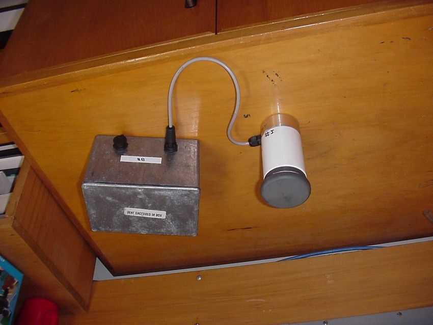
4                                                         Weather and Climate, 25

depend on the sixth moment of the raindrop size distribution whereas
rainfall rate is proportional to the diameter to the third power times the fall
speed of the raindrops. Therefore, knowledge of the raindrop size distribu-
tion at the time of measurement is important if an accurate estimation of the
rainfall rate is to be made from radar measurements. In recent years, the
Joss-Waldvogel (1967) Disdrometer (JWD) has been the only widespread
automatic device to measure raindrop size and, therefore, raindrop spectra.
As the cost of a single JWD unit can be prohibitive (at least in New Zealand)
the study of raindrop spectra has not advanced as far as it could have -
even though many types of automatic disdrometer systems have been
developed.
        The disdrometer project within the Atmospheric Group at the
University of Auckland has two main aims. The first is to develop a relatively
inexpensive and reliable disdrometer system to complement the current
equipment already used in the Atmospheric Group at the University of
Auckland. This includes a very high space time resolution radar system, a
dense gauge network and meteorological towers. The development of a
reliable disdrometer system is non-trivial, as there can be many and various
sources of error (largely electrical and environmental), that can cause
results to be compromised. Secondly, to then use the disdrometer(s) to
discover some basic relations in the raindrop spectra not only for individual
rain events, but also for different synoptic conditions. It is hoped that with
the construction of up to half a dozen disdrometers, used together in
conjunction with a dense raingauge network and a high resolution X band
radar, that the study of raindrop spectra in relation to dual Z – R measure-
ments can be advanced along paths that up until now have not been tried.
The new disdrometers were designed with the following criteria in mind:
    •   to be cost effective
    •   to be rugged enough to last in extreme conditions
    •   to be easy to repair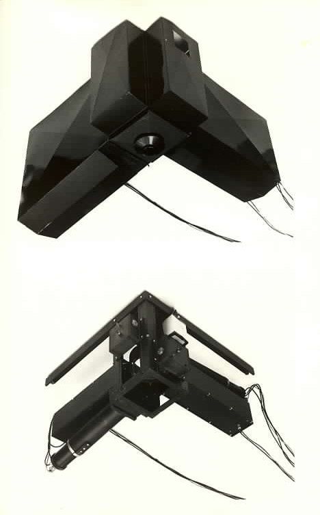
Henson and Austin: Raindrops and Disdrometers                                   5

    •    to be portable, i.e. have its own power supply
    •    that the power supply be able to last for at least 2 days continuous
         use
    •    that the memory storage be able to last for at least 2 days continu-
         ous use
    •    that we maximise the range of diameters that can be measured
    •    that the accuracy in the bulk quantities are maximised
Even though some of these criteria are ambitious, if the construction of the
new disdrometers was based around piezo-ceramic transducers then it was
felt that all of these general criteria could be met, based on the work of
Camilleri (2000).

What is a Disdrometer?
        A disdrometer is a device that measures the distribution of the sizes
of individual raindrops. While there are several types of disdrometers, they
all measure raindrop sizes using different principles and different measuring
methods. The two main types of disdrometer systems are optical disdrome-
ters and impact disdrometers. Optical disdrometers rely on raindrops cross-
ing a beam (or beams) of light. The raindrop size is determined from the
“shadow” the raindrop creates, from the amount of light scattered or is
inferred from the velocity of the raindrop. These types of disdrometers are
typically quite large and unwieldy, as the sample volume through which a
raindrop has to fall tends to be quite large. Impact disdrometers measure
the raindrops’ momentum as it impacts on the surface area of the instru-
ment.
        At the moment, there is essentially only one commercially available
impact disdrometer: the Joss-Waldvogel disdrometer. It uses the raindrop
momentum to push down a lightweight cone and, using induction coils,
thereby induce a measurable voltage. As the cone is made of polystyrene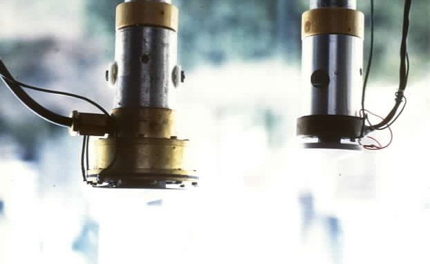
6                                                            Weather and Climate, 25

with an aluminium covering and moving parts, it is not a particularly sturdy
device. With a price tag in the region of $20-25,000 USD, it is more
expensive than the entire Auckland University radar system (which is
discussed a little bit later on).
        The disdrometer systems developed by the University of Auckland
use piezo-ceramic discs and piezo-hydrophones, typically used to detect
underwater noise. These transfer the momentum of the raindrop into a
voltage signal. As well as being relatively inexpensive, this method of
measuring the raindrop size has the advantage of being sturdy and reliable.
The challenge is to make the performance of the piezo-electric/hydrophone
system comparable to the commercially available Joss-Waldvogel disdrom-
eter.

Why Use a Disdrometer?
        The University of Auckland’s Atmospheric Group’s main hardware is
an X-band radar (shown below in Figure 1) that is mounted on a caravan for
portability. This allows it to access locations where the larger Meteorological
Service radars cannot operate. Radars can detect and measure the reflec-
tivity of a rain cell, but they can not reliably predict the amount of rainfall that
occurs at ground level.
        Only a disdrometer can measure the rainfall rate to radar reflectivity
relationship simultaneously at ground level during a rain event - this relation-
ship is dependant on the raindrop size distribution. Therefore, if a radar and
a disdrometer are used together, the rainfall over a wide area can be
calculated (assuming homogeneity of the rain cell). One question would still
remain, and that would be due to the error introduced by using the incorrect
values for the Z – R relationship as the disdrometer measures rainfall
effectively at a point and a radar measures rainfall over a large area. The
error in the accumulation as measured by a radar due to sampling errors
alone was examined in Fabry et. al. (1994). It was found in Fabry et. al.
Henson and Austin: Raindrops and Disdrometers 7
Figure 1. The Auckland University X-Band Mobile Radar
(1994) that the sampling errors were relatively large even at short temporal
and spatial resolution (see Figure 2). For information about the assumptions
made in the simulation Fabry performed, Fabry et. al. (1994) should be
referred to. By using the data a disdrometer provides it would be possible to
examine how much additional error is introduced by using a Z – R relation-
ship that deviates away from the optimum relationship, as calculated by the
data. This would give an indication as to the level of accuracy to which the Z
– R relationship would need to be stated.
There has been considerable discussion in the literature (Sekhon and
Srivastava, 1971; Waldvogel, 1974; Ulbrich, 1983; Feingold & Levin, 1986;
Willis & Tattleman, 1989; Tokay, et. al. 1999) about the relationship between
raindrop size distribution and the meteorological physical process that is8 Weather and Climate, 25 Figure 2. Absolute error in 5Min accumulations as a function of the resolu- tion of the reflectivity maps and sampling intervals. From Fabry et. al. 1994. occurring. Raingauges and radars only measure the various moments of the raindrop size distribution. The exact shape of the spectra is not easily inferred from these measurements, unless a specific distribution is as- sumed. Also, if there is a model that can predict (on average) raindrop- raindrop interactions as a function of height, then it is relatively easy to calculate what the raindrop size distribution is at various heights. This would be a useful comparison to vertically pointing radar (VPR) measurements
Henson and Austin: Raindrops and Disdrometers                                 9

and would give an idea of conditions aloft. As the amount of energy liberated,
as latent heat in a rainfall event is an order of magnitude greater that the
energy needed to generate a moderate wind, this knowledge can be crucial
in understanding the weather as a whole. The importance of rainfall in the
atmospheric processes can be seen in Browning (1990).
       Another use for disdrometers is to estimate the amount of soil erosion
or crop damage that occurs during a rain event. The amount of soil erosion
is proportional to the kinetic energy of a raindrop, which is approximately
                   4
proportional to D . However, this area of use for disdrometers is not well
known and few papers have been published into the use of disdrometers in
this area.

The History of Measuring Raindrops and the Drop Size
Distributions
       One of the earliest papers on measuring raindrops was published by
E. J. Lowe in 1892. In his paper he describes using slabs of slate, where
raindrops would impact on the slate and the impact patterns would be copied
onto sheets of paper. In his paper, Lowe hypothesised that large raindrops
were hollow. During the discussion, after the paper was presented, it can be
noted that a certain Mr. Whipple suggested the use of chemically treated
paper instead of slabs of slate. There was some discussion as to whether it
was Whipple or M. Hervé-Mangon who originally suggested the idea. Not
long after, Wiesner (1895) used absorbent paper, where raindrops strike the
paper and leave stains. The stains would be measured and the raindrop size
inferred. This appears to be the first time using absorbing or dyed filter paper
was used.
       Around this time Wilson Bentley (1904) used trays of flour and
measured the different sizes of raindrops from different parts of a storm. In
this method trays of deep uncompacted flour with a smooth surface were
10 Weather and Climate, 25
exposed to rain. Raindrops would form a dough pellet that hardened after
the trays were baked and the size of the pellets corresponded to the size of
the raindrops. Bentley noted that raindrop sizes varied dramatically at times
between the different parts of the storm, depending on the conditions. At the
same time Von P. Lenard (1904) published what is possibly the most
comprehensive study of raindrops for the period, using the absorbent paper.
It includes measured values for the raindrops’ terminal velocities, the
required wind velocity to keep raindrops aloft and a discussion of raindrop to
raindrop collisions. Raindrop sizes for ten storm events (from September
1898 till July 1899 in northern Germany) are also provided along with
observations on the conditions. Raindrop sizes had previously been
grouped as small, medium, large, etc., but this extensively detailed paper
contained the actual sizes of the raindrops. Albert Defant also used the
absorbent paper method in 1905 and from his data suggested that the
weight of raindrops tended to be in the ratio 1:2:4:8.
Spencer Russell (1911) used both the slabs of slate and trays of
plaster of Paris (similar to using trays of flour) to determine the sizes of
raindrops from many different types of cloud structures. There was a
discussion following the presentation of the paper and it was mooted that
Defant’s data suggested that raindrops grew while falling - with the smaller
raindrops combining to form larger ones. There was then some interest
th
whether or not Russell’s data supported this view. By the turn of the 20
century it is clear that scientists were coming to the conclusion that
raindrops interacted with each other and coalesced.
It is likely that Schindlehauer (1925) constructed the first electronic
disdrometer. The principle used was that a raindrop hits a diaphragm
causing air to blow through a whistle. The resultant noise was recorded
using a microphone. A schematic diagram of the disdrometer is shown in
Figure 3. According to Schindlehauer (1925), his disdrometer worked well
except for small drops and snow, although no data was published in theHenson and Austin: Raindrops and Disdrometers 11
paper. Niederdorfer (1932) published a paper containing a calibration curve
for using a particular type of dyed paper. The paper was quite detailed (far
Figure 3. Schematic diagram of Schindlehauer disdrometer.
more so than anyone else to date) recording raindrop sizes for eight rain
events. These events were commented on in some detail and Niederdorfer
concluded that some raindrop sizes prevailed over others and that, since
his data was taken at three geographically different areas, the meteorologi-
cal processes were the same at all three sites.
Using filter paper was the primary method of measuring raindrop
sizes until the 1950s. At that time various machines were constructed, using
a variety of methods, to calculate the size of a raindrop. Some of these
methods include a variation of using filter paper (Sivaramakrishnan, 1961),
where filter paper is continuously exposed using a roller system and then
dried and stored. Another machine that was used, was constructed having12 Weather and Climate, 25 finely spaced wires as the “collection area”. In order for a measurement to be made a raindrop was required to hit two wires, thereby closing the connection and conducting a current. Unfortunately, the portability of the filter paper machine was limited and the wire machine had resolution problems. In the 1960s optical disdrometers were in their infancy and it was not until 1969, with the development of the Joss-Waldvogel RD-69 Dis- drometer (see Figure 4), that a standard disdrometer system was available for use. The Joss-Waldvogel disdrometer (Joss & Waldvogel, 1967) con- Figure 4. Schematic of Joss-Waldvogel Disdrometer from Joss and Wald- vogel (1967).
Henson and Austin: Raindrops and Disdrometers                             13

sists of a styrofoam body covered by an aluminium surface which, when a
raindrop impacts on the surface, causes a downward displacement and a
voltage is induced in a set of coils. The Joss-Waldvogel disdrometer is still
the most widely used disdrometer system today.
        There are two other disdrometer systems that have begun to be
widely used since the early 1990s. One of those is the disdrometer
developed by John Hopkins University (known as the JHU/APL disdrome-
ter, see Figure 5). This is the successor of the disdrometer as found in a
paper published by Rowland (1976). The JHU/APL disdrometer was based

Figure 5. Crossectional view of JHU/APL disdrometer.
14 Weather and Climate, 25
on a piezoelectric transducer that was under a Delrin plug. Raindrops would
strike the Delrin plug, compressing the piezoelectric transducer thereby
generating a voltage. Unfortunately, this disdrometer did not perform well
and production was discontinued.
The other disdrometer beginning to be widely used is the 2D-video disdrom-
eter developed by Joanneum Research in Graz, Austria (Figure 6). This
disdrometer can not
only measure the size
of raindrops (both hori-
zontally and vertically)
but also its terminal ve-
locity, shape and
phase of the raindrop.
The 2D-video disdrom-
eter utilises two video
cameras at right an-
gles to take simultane-
ous images of hydrom-
eteors. It is from these
images that the various
quantities can be in-
ferred. More informa-
Figure 6. Photo of the 2D video disdrometer
tion can be found on
the 2D-video disdrom-
eter can be found in Nešpor et. al. (2000).
The 2D-video disdrometer does have its drawbacks. It is large
3
(approximately 1m and 130kg) and requires a 500W power supply, its
outdoor electronics unit is prone to overheating, it creates a large amount of
data (several hundred Mb in a few hours), it has problems with its optical
path being obscured, its optics can be knocked out of alignment and it canHenson and Austin: Raindrops and Disdrometers 15
suffer system lockups (and therefore a loss of data) from a variety of
reasons (high rainrates, midnight rollover, etc.). It would seem that most of
these problems could be overcome in the future as they are either relatively
trivial or with the advance of technology new devices will solve the problems.
The most recent disdrometer that has come onto the market is the
WXT510 Weather Transmitter from Vaisala. The Vaisala Weather Transmit-
ter offers a set of six weather instruments in a single device. It is apparently
easy to install and has no moving parts. The precipitation sensor converts
impacts from single raindrop impacts into voltage signals. However, at this
point it is unclear exactly how the Vaisala Weather Transmitter operates as
this instrument is very new and the authors have not seen this device or read
any reports on it. More information about this new instrument can be found
on the Vaisala website.
One novel approach of measuring the raindrop size distribution is to
use a body of water as the effective collection area. When a raindrop of
specific size travelling at its terminal velocity hits a body of water, a small
bubble is created. This bubble collapses and a “scream” is generated and
can be analysed with a hydrophone. This “scream” has a frequency that is
distinct enough that it can be distinguished from other noise including the
crashing of waves (if in the ocean). If the intensity of the “scream” created by
rainfall is measured, then the number of raindrops that create this sound can
be determined. This approach has one big advantage in that the deeper the
hydrophone, the greater the effective collection area. This means that a
large body of water such as a swimming pool, or even lakes could be used
to measure rainfall. The only drawback is that the range of raindrops that are
able to create this “scream” is relatively small and in general a raindrop size
distribution shape has to be assumed. For more information about this
technique there are many papers that could be investigated. Nystuen (1986)
and Pumphrey and Crum (1989) and are two such papers and more recently
Quartly et. al. (2002) which also examines other buoy-mounted rainfall16 Weather and Climate, 25
instruments.
Raindrop Size Distributions
During the Second World War, Laws and Parsons (1943) produced their pa-
per relating raindrop size distributions to rainfall intensity. Not long after,
Best (1947) also published his paper relating rainrate to the fraction of liquid
water in the air. These two relations, while not strictly raindrop size distribu-
tions, set some bounds on what the possible distribution could be. It was not
until 1948 that Marshall and Palmer formulated the first raindrop size distri-
bution. The Marshall-Palmer distribution, as it became known, related the
raindrop size distribution to the rainfall rate and the radar reflectivity - devel-
oping the first Z – R relationship based on a raindrop size distribution. A re-
production of the data presented in Marshall and Palmer (1948) can be seen
in Figure 7. The Marshall-Palmer distribution is described by the general re-
lation
N (D ) = N o e − Λ D
where D is the drop diameter in units of mm, N(D)∆D is the number of
drops in the range D to D+∆D, and No is the value of N(D) for D=0. The value
for No is usually stated as
N o = 0 . 08 cm − 4 = 8000 m − 3 mm − 1
And the relation between Λ and the rainrate R is
Λ = 41 R − 0 .21 cm − 1 = 4 . 1 R − 0 .21 mm − 1
This gave a theoretical Z – R relationship of
Z = 296 R 1.47
If a random variable X is normally distributed, then Y=ln(X) is log-
normally distributed, and therefore the probability density function of x isHenson and Austin: Raindrops and Disdrometers 17
Figure7. Figure from Marshall and Palmer (1948) showing data at Ottowa
in 1946 (dotted lines), the results from Laws and Parsons (broken lines)
and the MP distribution (solid straight lines).
1 (ln (x ) − µ )2
f (x; µ , σ ) = exp −
σ 2π x 2σ 2
The raindrop size distribution can therefore be parameterised as
NV (ln (D ) − µ )2
N (D ) = exp −
σ 2π D 2σ 2
3
Where Nv, σ and µ are the number of raindrops in a 1 m sample volume,
the standard deviation and mean of the natural logarithms respectively.
These quantities are easily calculated to give an analytic solution, if a18 Weather and Climate, 25
power-law relationship for the raindrop terminal velocity is assumed. It is
extremely difficult to calculate these quantities if the Atlas et. al. (1973)
version of raindrop terminal velocity is assumed.
Feingold and Levin (1986) have also written the lognormal distribu-
tion as
ln 2 D
NT D
N (D ) = exp − g
2
2 ln σ
2
2π ln σ D
Where NT , σ and DG are the raindrop concentration (equivalent to NV
above), standard geometric deviation (standard deviation of the log of the
diameters) and mean geometric diameter respectively (or median raindrop
size).
The commonly used form of gamma distribution is that given by
Ulbrich (1983, 1985) and it is
N (D ) = N G D µ −1 exp (− Λ D )
The term µ is often referred to as the shape parameter and Λ as the scale
parameter. The gamma distribution can be rewritten in terms of NV, the
3
number of raindrops in a 1m sample volume (as done in the lognormal
distribution above), and then it becomes
N V Λµ µ −1
N (D ) = D exp (− Λ D )
Γ (µ )
It can readily be seen that if µ=1, then the gamma distribution simplifies to
the Marshall-Palmer distribution and the scale parameter is the same as the
one given by the Marshall-Palmer distribution. It has also been experimentallyHenson and Austin: Raindrops and Disdrometers 19
shown by Ulbrich (1983) that NG was found to have been related to µ by the
relation
N G = 6 × 10 4 exp (3 . 2 µ ) m -3 cm -1- µ
or
N G = 1 .5 × 10 4 exp (3 .14 µ ) m -3 cm -1- µ
The difference between the two relations is thought to be due to spatial av-
eraging.
It was the period following the development of the Joss-Waldvogel
Disdrometer that the greatest advancement on parameterizing raindrop size
distributions was made along with the introduction of the gamma and
lognormal distributions. Several other raindrop size distributions were postu-
lated in the 1950’s, however all of these were special cases of the gamma
and lognormal distribution, or they fell into disuse due to their complicated
form.
In terms of radar meteorology, it is the large raindrops that hold the
most importance. This is due to the fact that the rainrate is proportional to
the diameter to the power of approximately 3.5 and the radar reflectivity is
proportional to the diameter to the power 6. Therefore, it is easy to see that
a relatively few large raindrops will have more significance than many
smaller raindrops.
At the large raindrop size, the gamma and lognormal raindrop size
distribution described above tend toward an exponential (and therefore
Marshall-Palmer) distribution. This was certainly the case with all the data
taken during the field trials of the disdrometer developed by Henson (2002)
as can be seen in Figure 8 as an example. This is undoubtedly why the
relatively simple Marshall-Palmer distribution is still so widely used today
even though it clearly overestimates the number of small raindrops. The20 Weather and Climate, 25
minimum raindrop size for the data taken in Figure 8 was 0.8mm diameter.
However, this was subsequently improved to approximately 0.6mm diame-
ter and this value was set at start-up in software. The minimum raindrop size
measured by this disdrometer system was limited due to noise problems
caused by the piezo-ceramic oscillating in a planar mode, but this could be
solved with a different choice of piezo-ceramic crystal. More information
about the performance of this disdrometer system can be found in Henson
(2002) or in Henson et. al. (2004).
th
Figure 8. Raindrop Size Distribution taken on 4 of September 2001 at
Auckland University Ardmore field site.Henson and Austin: Raindrops and Disdrometers 21
The Development of Disdrometers at the University of
Auckland
The University of Auckland has a rich and innovative history when it
comes to measuring raindrops and raindrop size distributions. To date there
have been four PhD programs: Larsen (1970), Bradley (1975), Camilleri
(2000) and Henson (2002) and three MSc programs: Bradley (1971), Jones
(1979) and Webb (2000), solely in the construction or use of disdrometers.
These PhD and MSc programs have produced many papers to scientific
journals (too many to name here). In addition to disdrometers, a mobile
X-band radar has been built and successfully used and is described in Nicol
(2001), with a more modern version in construction. The University of
Auckland has also produced drop counting “Hydra” gauges, described in
Hosking et. al. (1986). This shows the variety of skills in both the technical
and academic expertise that has been present at the University of Auckland
over the years.
A brief description of those PhD and MSc theses, which deal solely
with disdrometers or the measurement of the raindrop size distributions, will
now be looked at in turn.
1. Larsen (1970)
This disdrometer was primarily designed to measure the charge
distribution of raindrops. It utilised a charge induction cylinder and
was small enough that it could be mounted such that it swivelled in
windy conditions. Therefore raindrops would fall directly down the
cylinder. Raindrop sizes were also measured using a light scatter-
ing technique. A photograph of this disdrometer can be seen in
Figure 9 and more information about this disdrometer can be found
in Larsen (1970).
2. Bradley (1971 & 1975)
Similar to the disdrometer used by Larsen, this disdrometer also22 Weather and Climate, 25
measured the charge distribution of raindrops using an induction
cylinder and measured the raindrop sizes using a light scattering
technique. However, unlike the disdrometer used by Larsen, this
disdrometer was mounted on a stand so was immovable. A de-
scription of this disdrometer can be found in Bradley and Stow
(1974).
3. Jones (1979)
This was an optical disdrometer that used the amount of light that a
raindrop will scatter as it passed through a light beam. Unfortu-
nately, this disdrometer was quite large (approximately 1m in
length) and therefore suffered from portability problems, required
mains power and more importantly could not be used outdoors. A
photograph of this disdrometer can be seen in Figure 10 and more
information concerning this disdrometer in Jones (1979).
4. Webb (2000)
Webb developed an instrument that used ultrasound to remotely
sense raindrop size distributions. This instrument emits short
acoustic pulses into the atmosphere and measures the Doppler
spectrum of the sound reflected back from the raindrops. The
Doppler shift is proportional to the terminal velocity and gives an
estimate of the raindrop diameter. The intensity of scatter as a
function of the Doppler frequency shift gives a measure of the
number of raindrops of each diameter. This technique is similar to
that used by the POSS system described by Sheppard (1990).
More information about this disdrometer can be found in Webb
(2000).
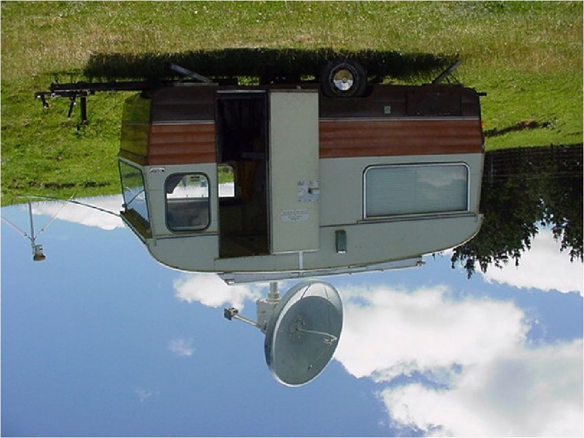
5. Camilleri (2000)
A rugged impact disdrometer developed using ex-Navy hy-
drophones. Raindrops would strike an aluminium cap, compressing
the hydrophone and inducing a voltage. The raindrop diameter wasHenson and Austin: Raindrops and Disdrometers 23
then estimated from calibration data. However, this disdrometer
required a computer and mains power so was not completely
portable. Additionally, since the design was based on ex-Navy
hydrophones, construction of new disdrometers was difficult due to
scarceness of parts.
6. Henson (2002)
The disdrometer produced in Henson (2002) was in essence a
follow-on from the Camilleri disdrometer. The new disdrometer
system was constructed almost entirely out of PVC and used
lead-acid gel cell batteries to power a microprocessor. Therefore,
compared to the many disdrometer systems developed previously,
this new system is completely portable and does not suffer from
electrical mains noise or heating problems. The sensor unit is based
around piezo-ceramic disks and operates in essentially the same
manner as the Camilleri disdrometer described above. However,
the sensors are commercially available so parts for new disdrome-
ters could be easily obtained. The total cost of parts for this
disdrometer system was conservatively estimated at $1000 NZD.
More information about this disdrometer can be found in Henson
(2002) or in Henson et. al. (2004).24 Weather and Climate, 25
Figure 9.
Figure 10.
Disdrometer
Disdrometer
used by
used by
Larsen
Jones (1979)
(1970)
Figure 11. Disdrometers used by Camilleri (2000)
Figure 12. Disdrometer used by Henson (2002)Henson and Austin: Raindrops and Disdrometers 25
The Future of Disdrometers
The measurement of raindrops and raindrop size distributions has not
had an easy history. The range of measurements required, from the smallest
raindrop to the largest, for any particular measurement technique can often
put unrealistic constraints on the equipment. There are also errors which can
cause considerable difficulties for both the equipment or the collectors of the
data. The advent of microprocessor technology (or improvement of technol-
ogy in general) has made a significant improvement to the way raindrops are
measured as disdrometers can now be stand-alone, portable and cost
effective. This means that they can be placed anywhere and more than one
can be used in a variety of possible configurations.
The future of disdrometers would appear to be bright. There are a
number of projects around the world working on either optical or impact
disdrometers. Three of these (not including those from the University of
Auckland and those previously mentioned) are impact disdrometers in
Jayawardena & Rezaur (2000), Förster (1994) and an optical disdrometer in
Lavergnat & Golé (1998). With the increasing number of projects and the
continual advancement of technology (video, microprocessors, etc) this can
only make the availability and use of disdrometers more widespread. It will
also increase the understanding of raindrops and the processes that they
influence, or interact with, and give us a better picture of the energy balance
in the atmosphere. This should prove invaluable to modellers as this infor-
mation can be scarce on a localised scale. While radar and satellite pictures
will undoubtedly provide a greater understanding of rain events over a wide
area, the use of disdrometers, in conjunction with radar, provides a link
between what is occurring at the ground and what happens aloft. This is
likely to continue to be the primary use of disdrometers.26 Weather and Climate, 25
References
Atlas D., Srivastava R. C. and Sekhon R. S., 1973: Doppler Radar Charac-
teristics of Precipitation at Vertical Incidence. Rev. Geophys. Space Phys.,
11, 1-35.
Bentley W. A., 1904: Studies of Raindrops and Raindrop Phenomena. Mon.
Weath. Rev., 32, 450-456.
Best A. C., 1947: The size distribution of raindrops. Met. Res. Pap., 352,
London.
Bradley S. G., 1971: A study of distribution of raindrop size and charge. PhD
Thesis, University of Auckland.
Bradley S. G., and Stow C. D., 1974: The measurement of charge and size
of raindrops. I. The disdrometer. J. Appl. Meteor., 13, 114-130.
Bradley S. G., 1975: Physical and electrical properties of raindrop interac-
tions. PhD Thesis, University of Auckland.
Browning K. A., 1990: Rain, rainclouds and climate. Quart. J. Roy. Meteor.
Soc., 116, 1025-1051.
Camilleri M., 2000: Sampling Errors in the Measurement of Rainfall. PhD
Thesis, University of Auckland.
Fabry F., Bellon A., Duncan M. R., and Austin G. L., 1994: High Resolution
Rainfall Measurements by Radar for Very Small Basins: The Sampling
Problem Re-examined. J. Hydrol., 161, 415-428.
Feingold G. and Levin Z., 1986: The Lognormal Fit to Raindrop Spectra from
Frontal Convective Clouds in Israel. J. Appl. Meteor., 8, 249-253.
Förster J., 1994: Rain Measurement on Buoys Using Hydrophones. IEEE J.
Ocean. Eng, 19, 23-29.
Henson W. L., 2002: Development of a Low Cost Disdrometer System and
Disdrometer Observations of Storm Events. PhD Thesis, University of
Auckland.
Henson W., Austin G. and Oudenhoven H., 2004: Development of an
Inexpensive Raindrop Size Spectrometer. J. Atmos. Oceanic Technol., 21,
1710–1717.
Hosking J. G., Stow C. D., Bradley S. G. and Gray W. R., 1986: An improved
high-resolution raingage. J. Atmos. Sci., 3, 536-41.
Jayawardena A. W. and Rezaur R. B., 2000: Measuring Drop Size Distribu-
tion and Kinetic Energy of Rainfall Using a Force Transducer. Hydrol.
Process., 14, 37-49.
Jones K., 1979: A self-evaluating disdrometer. MSc Thesis, University of
Auckland.
Joss J. and Waldvogel A., 1967: Ein Spektrograph für Niederschlagstropfen
mit automatischer Auswertung. Pure Appl. Geophys., 68, 240-246.
Larsen H. R., 1970: The electric charge on raindrops. PhD Thesis, Univer-
sity of Auckland.Henson and Austin: Raindrops and Disdrometers 27
Lavergnat J. and Golé P., 1998: A Stochastic Raindrop Time Distribution
Model. J. Appl. Meteor., 37, 805-818.
Laws J. O. and Parsons D. A., 1943: The Relation of Raindrop-Size to
Intensity. Trans. Amer. Geophys. Union., 24, 452-460.
Lenard P., 1904: Über Regen. Meteor. Z., 21, 248-262.
Lowe E. J., 1892: Rain Drops. Quart. J. Roy. Meteor. Soc., 18, 242-245.
Marshall J. S. and Palmer W. McK., 1948: The Distribution of Raindrops
With Size. J. Meteor., 5, 165-166.
Nešpor V., Krajewski W. F. and Kruger A., 2000: Wind-Induced Error of
Raindrop Size Distribution Measurement Using a Two-Dimensional Video
Disdrometer. J. Atmos. Oceanic Technol., 17, 1483-1492
Nicol J. C., 2001: High-resolution rainfall measurements using a portable x-
band radar system. PhD Thesis, University of Auckland.
Niederdorfer E., 1932: Messungen der Größe der Regentropfen. Meteor.
Z., 49, 1-14.
Nystuen J. A., 1986: Rainfall Measurements Using Underwater Ambient
Noise. J. Acoust. Soc. Am., 79, 972-982.
Pumphrey H. C. and Crum L. A., 1989: Underwater Sound Produced by In-
dividual drop impacts and Rainfall. J. Acoust. Soc. Am., 85, 1518-1526.
Quartly G. D., Guymer T. H. and Birch K. G., 2002: Back to basics: Measur-
ing rainfall at sea: Part 1 – In situ sensors. Weather, 57, 315-20
Rowland J. R., 1976: Comparison of Two Different Raindrop Disdrometers.
th
Preprints of Papers, 17 Radar Meteorology Conf., Seattle, Amer. Meteor.
Soc., 398-405.
Russell S. C., 1911: Raindrop Experiments. Quart. J. Roy. Meteor. Soc.,
11, 337-339.
Schindlehauer F., 1925: Versuch einer Registrierung der Tropfenzahl bei
Regenfällen. Meteor. Z., 42, 25-27.
Sekhon R. S. and Srivastava R. C., 1971: Doppler Radar Observations of
Drop-Size Distributions in a Thunderstorm. J. Atmos. Sci., 28, 983-994.
Sheppard B. E., 1990: Measurement of Raindrop Size Distributions Using a
Small Doppler Radar. J. Atmos. Oceanic Technol., 7, 255–268.
Sivaramakrishnan M. V., 1961: Studies of raindrop size characteristics in
different types of tropical rain using a simple raindrop recorder. Indian J.
Meteor. Hydrol. Geophys., 12, 189-216.
Tokay A., Short D. A., Williams C. R., Ecklund W. L. and Gage K. S., 1999:
Tropical Rainfall Associated with Convective and Stratiform Clouds: Inter-
comparison of Disdrometer and Profiler Measurements. J. Appl. Meteor.,
38, 302-320.
Ulbrich C. W., 1983: Natural Variations in the Analytical Form of the
Raindrop Size Distributions. J. Appl. Meteor., 22, 1764-1775.
Ulbrich C. W., 1985: The Effects of Drop Size Distribution Truncation on
Rainfall Integral Parameters and Empirical Relations. J. Appl. Meteor., 24,
580-590.28 Weather and Climate, 25 Waldvogel A., 1974: The Jump of Rain Spectra. J. Atmos. Sci., 31, 1067-1078. Webb T., 2000: The design and testing of an ultrasonic disdrometer for the remote sensing of rainfall . MSc Thesis, University of Auckland. Wiesner, J., 1895: Beiträge zur Kenntnis des tropischen Regens. Sitz. Ber. Math. Nat. Akad. Wiss. Kl. Wien, 104, 1397-1434. Willis P. T. and Tattelman P., 1989: Drop-Size Distributions Associated with Intense Rainfall Drops. J. Appl. Meteor., 28, 3-15. Ziegler D. W., 1987: War, Peace and International Politics. Little, Brown and Co., New York, 444pp. Submitted to Weather and Climate July 2003, revised December 2004
You can also read