Green Energy for a Green City-A Multi-Perspective Model Approach - MDPI
←
→
Page content transcription
If your browser does not render page correctly, please read the page content below
sustainability

Article
Green Energy for a Green City—A Multi-Perspective
Model Approach
Jarosław Watróbski
           ˛       1, *, Paweł Ziemba 2 , Jarosław Jankowski 3 and Magdalena Zioło 4

 1   Faculty of Computer Science and Information Systems, West Pomeranian University of Technology,
     Zolnierska 49, 71-210 Szczecin, Poland
 2   Department of Technology, The Jacob of Paradyż University of Applied Science, Chopina 52,
     66-400 Gorzów Wielkopolski, Poland; pziemba@pwsz.pl
 3   Department of Computational Intelligence, Wrocław University of Technology, Wybrzeże Wyspiańskiego 27,
     50-370 Wrocław, Poland; jaroslaw.jankowski@pwr.edu.pl
 4   Faculty of Management and Economics of Services, University of Szczecin, Cukrowa 8, 71-004 Szczecin,
     Poland; magdalena.ziolo@wzieu.pl
 *   Correspondence: jwatrobski@wi.zut.edu.pl; Tel.: +48-91-449-5668

 Academic Editor: Andrew Kusiak
 Received: 22 May 2016; Accepted: 14 July 2016; Published: 26 July 2016

 Abstract: The basis for implementing demands for a green city is the use of, among other things,
 innovative “clean” technologies. However, it is mostly and directly connected to the increased
 use of electric energy. Green transport is an appropriate example of this. By contrast, conventional
 sources of energy (e.g., based on coal) have a very negative impact on people and the environment.
 Therefore, this article mentions an attempt to solve a complex problem of employing renewable
 energy sources (RES) as an element of the “green city” system. The research was carried out on
 the basis of a feasibility study (decision game) for the location of a wind farm in the vicinity of the
 city of Szczecin, Poland. When constructing the decision models, multiple-criteria decision analysis
 (MCDA) methods were applied, especially analytic hierarchy process (AHP) and preference ranking
 organization method for enrichment evaluation (PROMETHEE).

 Keywords: renewable energy sources; RES; multiple-criteria decision analysis; MCDA

1. Introduction
     Green cities are defined as cities characterized as having clean air and water, running a low risk
of major infectious disease outbreaks, being resilient to natural disasters, encouraging green behavior,
and having a relatively small ecological impact [1]. Therefore, green cities are related to, among other
things, renewable energy sources (RES), the use of which is environmentally friendly, minimizes
ecological influence and increases the quality of air in the city. The relationship between green cities
and renewable energy sources can be found in a report prepared by the European Green City Index, in
which 30 European capitals were evaluated in terms of their current environmental performance [2].
The ranking takes the following factors into consideration: air cleanliness, CO2 emission, a strategy
of CO2 reduction or the percentage of renewable energy in the total energy production [3]. Similarly,
Albino and Dangelico [4] noticed that the RES use is closely related to the philosophy of green cities
and is an essential practical aspect.
     Another element of green cities is environmentally friendly transport [3,5]. It is about, among
other things, supporting bicycle mobility, as is being done by municipal authorities of Polish cities,
such as in the city of Szczecin, by building bicycle paths and urban bicycle stations. Nevertheless, a
larger ecological potential for cities is the application of solutions used by a higher number of citizens
rather than the expansion of bicycle infrastructure. It is obvious that far more city dwellers use their

Sustainability 2016, 8, 702; doi:10.3390/su8080702                        www.mdpi.com/journal/sustainability
Sustainability 2016, 8, 702                                                                               2 of 22

own cars and public means of transport. Consequently, better results in terms of reducing pollution
emissions can be obtained by solutions such as electric or hybrid cars [6] as well as public transport
powered by electricity, i.e., trams and electric buses [7]. However, it should be noted that the use of
electric vehicles in the city causes increased demand for electric energy related to the necessity of
charging vehicle batteries. As a result, such a demand brings about the increase in energy production
from conventional sources, mostly from coal, even in cities where the power industry is to a great
extent based on RES [8]. Therefore, air pollution reduction resulting from the use of electric vehicles is
lower than is assumed [9]. The problem is even bigger, since almost all energy for the city is produced
by coal power plants. It may turn out that air pollution emission generated by a coal power plant
(resulting from the necessity of energy production for charging electric vehicles) is larger than the air
pollution emission when conventional vehicles are used instead of electrically powered vehicles [10].
Therefore, one cannot talk about a green city as long as it mostly relies on coal energy. Instead, energy
production technologies based on RES should be introduced more frequently.
     The use of RES as pro-environmental action is one of the main aims of the energy policy [11].
Renewable energy sources are the basic element of a low-carbon economy [12], and their percentage
in the total energy production is continuously increasing and will continue to increase in both the
European Union [13] and Poland [14,15]. On the other hand, the highest portion of energy production in
Europe [13] and Poland is supplied by wind turbines [15–17]. The Polish wind potential is comparable
to that of the “world wind giant” Germany and other countries in which a significant share of energy
is obtained from wind, such as Denmark or Sweden [18]. An inland wind turbine is distinguished by
lower capital spending and maintenance costs among RES, as seen in Table 1.

             Table 1. Capital spending and maintenance costs of renewable energy sources (RES) [19].

                                                      Capital Investment              Operational Costs
                    Energy Source
                                                         (€2005/kW)                     (€2005/kW)
              On-shore Wind                                   1140                             35
              Off-shore Wind                                  2000                             80
               Landfill Gas                                   1530                            200
               Biogas plant                                   3140                            245
          Hydropower—large scale                        1350, 1800, 2510                   40, 55, 75
          Hydropower—small scale                          2900, 4500                        85, 130
               Photovoltaics                                  4700                             80
         Concentrating Solar Power                            5000                            115
 Biomass combustion steam cycle—large scale                   2450                            135
 Biomass combustion steam cycle—small scale                   3800                            260

     The data show that wind is the most optimal renewable energy source. What is more, the highest
economic and market potential for wind energy in Poland (by 2020) is in West Pomeranian Province,
as depicted in Table 2. The economic potential was determined by considering arable lands in a
given province with appropriate wind conditions on which wind farms can be constructed. From
the potential investment areas, all areas subject to protection were excluded. These areas are national
parks, landscape parks, nature reserves, the Natura 2000 protected areas, areas of protected landscapes
and protected area buffer zones. The market potential (part of the economic potential that can be used
within a definite period of time) was calculated by means of a Modular Energy System Analysis and
Planning Environment (MESAP) model, as part of an Energy [R]evolution project, on the basis of
current market and political factors [20].
     The city of Szczecin plays an important role in the West Pomeranian region. The analysis of the
present energy policy of the city confirms that it is primarily based on a conventional source of energy;
that is, coal [21]. There are two coal power plants, “Pomorzany” and “Szczecin”, located in the city.
They significantly support the electric power grid during rush hours and therefore generate harmful
emissions in the city. The situation with regard to potential wind conditions and ecological limitations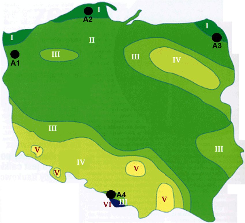
Sustainability 2016, 8, 702                                                                               3 of 22

seems to be unfavorable and is reflected in the Regional Innovation Strategy which emphasizes
the need for a continuous increase of the RES share in energy production, as presented by Urzad         ˛
Marszałkowski Województwa Zachodniopomorskiego [22]. An analysis of other economic and social
factors of the city also conveys substantial RES investment possibilities such as the use of technological
and social potentials of the city and the region as well as the availability of investment grounds; for
instance, neighboring districts that have low economic value but are also “good” locations for wind
farms, e.g., an area between the town of Goleniów and the northwest part of DabieLake
                                                                                    ˛         [23].

                         Table 2. Economic and market potential of wind energy in Poland [20].

            Province (Voivodeship)              Economic Potential (MW)           Market Potential (MW)
               West Pomeranian                           ~14,100                           ~3100
                  Pomeranian                             ~10,400                           ~1900
                  Lower Silesia                           ~9800                            ~300
              Warmian-Masurian                            ~7100                            ~300
                  Subcarpatian                            ~6700                            ~300
             Kuyavian-Pomeranian                          ~5200                            ~1500
                Greater Poland                            ~4100                            ~1400
                   Podlaskie                              ~4000                            ~800
                 Lesser Poland                            ~1800                             ~50
                      Opole                               ~1600                             ~50
                     Silesian                             ~1400                             ~50
                      Lublin                              ~1000                             ~50
                    Lubuskie                              ~500                              ~50
                Świ˛etokrzyskie                          ~200                             ~100
                       Łódz                               ~100                             ~100
                   Masovian                                ~50                              ~50

     The complex analysis of an RES investment location also requires a detailed analysis of the
technological potential of the city and the region. In Szczecin, and in the vicinity of the city, there are
many production companies related to wind energy. In Goleniów, LM Wind Power is manufacturing
rotor blades for wind turbines. In total, about PLN (Polish złoty) 600 million will be invested, which
is going to generate about 1400 jobs (currently 600) [24]. LM Wind Power also has a service center
in Szczecin, where approximately 140 workers are employed [25]. There is also KK Wind Solutions,
located in Szczecin, which produces wind turbine control systems. The company employs about
570 workers in the area of Szczecin [26,27]. As for the ability of investment to diversify an economically
unstable shipbuilding sector within the city, Bilfinger MARS Offshore serves as a prime example. This
company manufactures foundations for offshore wind farms, and over PLN 500 million were invested
to build the factory, which will employ about 500 workers [28].
     Apart from manufacturers of wind farm elements, an important part of a potential investment
process is planning and the realization of wind farm projects. Here, EPA-Wind, a Szczecin-based
company, should be mentioned. This company, which employs over 40 workers [29], deals with data
analysis, measurements, preparation and realization of wind energy projects. A Polish division of the
RP Global concern also has its registered office in Szczecin. RP Global Poland deals with the design,
implementation and maintenance of wind farms [30]. There are many business entities that act as
subcontractors and are responsible for constructing wind turbines. The detailed analysis of a broader
social context of investment makes us consider the social potential of the city. Wind energy investment
in the vicinity of Szczecin would also positively increase the number of workplaces related to wind
energy when investment preparation is concerned, as well as the management, maintenance and repair
of wind turbines. Estimates concerning the number of positions created by the wind energy sector are
presented in Table 3.
Sustainability 2016, 8, 702                                                                                   4 of 22

                              Table 3. Number of jobs created by the wind energy sector [31].

                                                            No of Jobs for 1 MW of      No of Jobs for 1 MW of
 Kind of Job                                                Wind Farm Power             Cumulated Wind Farm Power
                                                            Installed in a Given Year   Installed in a Given Year
 Production of wind farm elements—direct workplace                     7.5                           -
 Production of wind farm elements—indirect workplace                    5                            -
 Wind turbine installation                                             1.2                           -
 Management and maintenance of wind farms                               -                          0.33
 Other indirect workplaces                                             1.3                         0.07
 Total employment potential in the sector                              15                           0.4

     Furthermore, according to research for the European Commission, people employed in the RES
sector often come from other sectors where they had lost their jobs, such as the shipbuilding or steel
industries [32]. This observation is of utmost importance in the context of Szczecin, where the most
significant social problem has been the bankruptcy of one of the biggest employers, i.e., Szczecin
Shipyard, in 2002 [33].
     On the basis of the arguments presented above, one can state that the construction of wind farms
in the vicinity of Szczecin is very important, both for perceiving the city as a “green city” and for
social and economic reasons. Therefore, the aim of this paper is to identify conditions that should
take place so that a potential investor would chose the Szczecin region as a construction area of
wind farms. The aim is achieved by means of a kind of a decision game, which assumes that the
investor, who has several good locations for constructing wind farms, makes a decision with the use
of a multiple-criteria decision analysis (MCDA) method. Methodologically, the article presents an
attempt to build guidelines for using MCDA methods as a tool for identifying and constructing the
decision-maker’s preference model by maximizing the utility of a given decision variant. Such an
approach is a complement to possible plains of application of MCDA methodology in areas different
than classical problems of choice, ranking and sorting.

2. State of the Art
      Decisions related to RES ought to be seen as multiple criteria decision making problems with
correlating criteria and alternatives [34]. As far as RES decision problems are concerned, many criteria,
which are usually mutually conflicting, should be considered [35]. Often, a decision made in this field
is related to the necessity of taking into account different and contradictory interest groups [36,37].
This is because of complex relationships between technological, economic, environmental, ecological,
social and political conditions and aspects of the application of RES. Therefore, a natural tool for
supporting such decisions are MCDA methods [38]. This stems from the fact that MCDA methods can
provide a technical–scientific decision-making support tool that is able to justify choices clearly and
consistently, especially in the renewable energy sector [39,40].
      In the literature, one can find many examples of MCDA applications in the field of RES. These
methods are employed in order to: choose an energy production technology, analyze different scenarios
of RES development, optimize energy production, and evaluate RES-based power plants on the
environment or to select location for this kind of power plants. RES-related problems and MCDA
methods applied to solve the problems have been variously reviewed [34,36,41]. Research also deals
with the application of MCDA methods to wind energy; for example, Kaya and Kahraman [42] first
selected an energy production technology (wind energy received the highest mark), and then faced the
problem of finding a location for an on-shore wind farm working in the chosen technology. Lee, Chen
and Kang [43] presented the problem of location selection of an on-shore power plant and Watróbski,
                                                                                                ˛
Ziemba and Wolski [44] for an off-shore power plant. Moreover, Latinopoulos and Kechagia [45] as
well as Al-Yahyai et al. [46] based frameworks for location evaluation of on-shore wind farms on GIS
(Geographical Information System); Aydin, Kentel and Duzgun [47] presented a similar framework
for location evaluation of hybrid power plants, which use wind energy and solar-PV energy. Yeh and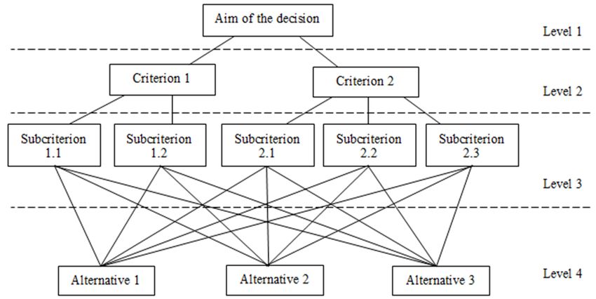
Sustainability 2016, 8, 702                                                                          5 of 22

Huang [48] determined criteria and their weights for the problematic of selection of a wind farm
location. Aras, Erdogmus and Koc solved another problem concerning the location selection of a wind
observation station [49]. Chang [50] considered a more complex problem presented in the selection of
specific energy production technologies and their locations. As for other decision problems, Cavallaro
and Ciraolo [40] carried out an evaluation of wind power plants designs. The designs were different in
quantity and power of wind turbines and were evaluated in terms of their suitability to one specific
location. Lozano-Minguez, Kolios and Brennan [51] evaluated foundations (truss) for off-shore wind
installations. Individual articles, along with their criteria and MCDA method are presented in Table 4.
Here, the criteria were divided into seven categories:

‚     technical aspects of the wind farm and its devices;
‚     spatial location of the farm with reference to surrounding area;
‚     economic issues especially ones related to the planned investment costs;
‚     social factors related to building and operating the wind farm;
‚     issues concerned with ecological aspects of the investment;
‚     environmental factors of the vicinity in which the farm is to operate; and
‚     legal articles and aspects related to the internal policy in terms of constructing wind farms.

      In Table 4, one can find out that the location evaluation of wind farms is often influenced by spatial
criteria, such as a distance from the road network and the power grid. Another frequent technical
criterion is the amount of generated energy. In the context of generated energy, the environmental
aspect is essential; i.e., wind speed, as it directly influences the amount of generated energy. Among
the economic criteria, the most crucial ones seem to be investment, operation and maintenance costs.
Social factors are also of importance; above all, the social acceptance of constructing a wind farm and
of changes to the surroundings. A basic ecological factor that is often mentioned among the criteria is
an estimated emission intensity reduction related to withdrawals from fossil fuels. The volume level
of wind turbines, the influence on protected area and distance from such areas are often listed among
the ecological factors.
      Lately, a dynamic development of MCDA methods has been observed. Both new methods
are created and well-known techniques are further developed. They are widely used in decision
problems related to, for instance, sustainable development, ecology or wind energy. In this area,
both European and American school decision-making methods are applied [52]. When analyzing
the literature, one can notice in order to solve decision problems related to wind energy, the analytic
hierarchy process (AHP) method is most often used. A generalization of the AHP method, in the
form of analytic network process (ANP), is also employed. The reasons for this are relatively simple:
computational algorithms for these methods and the possibility of hierarchical structurization of a
decision problem [43]. However, AHP/ANP methods are based on qualitative evaluations, therefore,
they do not make it possible to precisely present quantitative data. In decision problems related to
wind power engineering, other methods of the American decision-making school are also applied,
such as Technique for Order of Preference by Similarity to Ideal Solution (TOPSIS), Vlsekriterijumska
Optimizacija I KOmpromisno Resenje (VIKOR), simple additive weighting (SAW) or ordered weighted
averaging aggregator (OWA) and their developments using fuzzy number arithmetic [42]. As far as the
European decision-making school methods are concerned, ELimination Et Choix Traduisant la REalité
(ELECTRE) methods as well as the preference ranking organization method for enrichment evaluation
(PROMETHEE) method are often used [44]. These methods are especially used when a quantitative
data approach is applied. Independently, e.g., Latinopoulos and Kechagia [45], Al-Yahyai et al. [46] as
well as Yeh and Huang [48] attempted, successfully, to combine several methodological approaches.
The AHP (or also ANP) method is frequently used to determine a priority vector, whereas other
techniques (e.g., Decision Making Trial and Evaluation Laboratory (DEMATEL), OWA, and SAW) are
often employed in the aggregation process of final decision variants.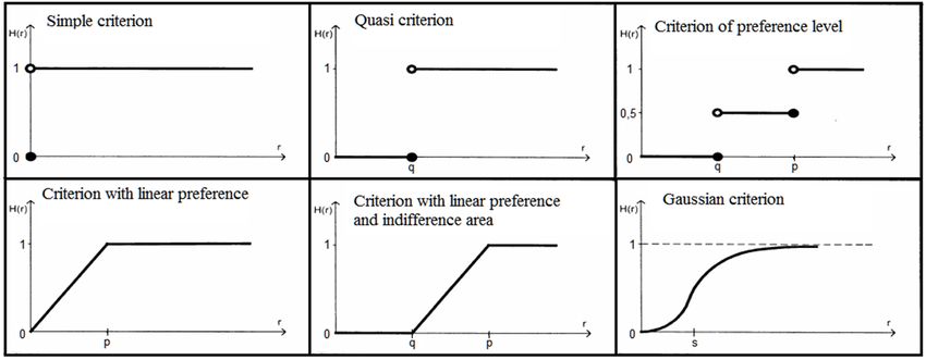
Sustainability 2016, 8, 702                                                                                                                                                                6 of 22

                                        Table 4. Application of multiple-criteria decision analysis (MCDA) methods in the field of wind Energy.

                                                                                         Main Criteria
                Decision Problem                   C                                                                                      NC            MCDA Method               Reference
                                                             Te        Ec         So         El          En        Sp          Po
  Selection of location for on-shore wind farm    SLo       TE       IC, OC     SA, VI    AN, IE                                          7     Fuzzy AHP + Fuzzy VIKOR              [42]
  Selection of location for on-shore wind farm    SLo      TE, TS    IC, OC      SC                  WS, GS                  RS, OS      25              AHP                         [43]
  Selection of location for off-shore wind farm   SLo       EP       IC, PT      SC         PA         GS         DE                     10          PROMETHEE II                    [44]
   Geographical Information System (wind)         SLo                                                SL, WS      DR, DP                   6            AHP + SAW                     [45]
       Geographical Information System                                                                                                 10—wind;
                                                  SLo                                       AN       SL, WS    DE, DR, DP                                OWA                         [47]
               (wind and solar-PV)                                                                                                     9—solar
   Geographical Information System (wind)         SLo                                                    WS        DR                     7           AHP + OWA                      [46]
     Key factors of location for wind farms       SLo        TS                 LB, VI      CR           WS        DR        RS, OS      15      Fuzzy DEMATEL + ANP                 [48]
            Selection of location for a
                                                  SLo                IC, OC       IA                     TB        DE                     13                  AHP                    [49]
            wind observation station
       Adjustment of energy production
                                                  SLo        EP      IC, OC     LB, SA      CR                                             7                 MCGP                    [50]
       technology for their best locations
          Selection of foundations for
                                                  TSl      TE, TS      NV                   CR           TB                                9                 TOPSIS                  [51]
           off-shore wind installations
        Abbreviations: AHP—analytic hierarchy process, AN—acoustic noise, ANP—analytic network process, C—category, CR—carbon reduction, DE—distance from the national energy
        connection, DEMATEL—decision making trial and evaluation laboratory, DP—distance from protected areas, DR—distance from road network, El—Ecological, Ec—Economic,
        En—Environmental, EP—energy production, GS—geology suitability, IA—infrastructure accommodation, IC—investment cost, IE—impact on ecosystems, LB—local benefits,
        MCGA—multi-choice goal programming, NC—number of criteria, NV—net present value, OC—operational cost, OS—other support, OWA—ordered weighted averaging aggregator,
        PA—influence on the protected areas, Po—Political, PROMETHEE—preference ranking organization method for enrichment evaluation, PT—payback time, RS—regulation for
        energy safety, SA—social acceptability, SAW—simple additive weighting, SC—social conflicts, SLo—site location, SL—Slope, So—Social, Sp—Spatial, TB—topography-natural barrier,
        Te—Technical, TE—technical efficiency, TOPSIS—technique for order of preference by similarity to deal solution, TS—technical safety, TSl—technology selection, VI—visual impact,
        VIKOR—vlsekriterijumska optimizacija i kompromisno resenje; WS—wind speed.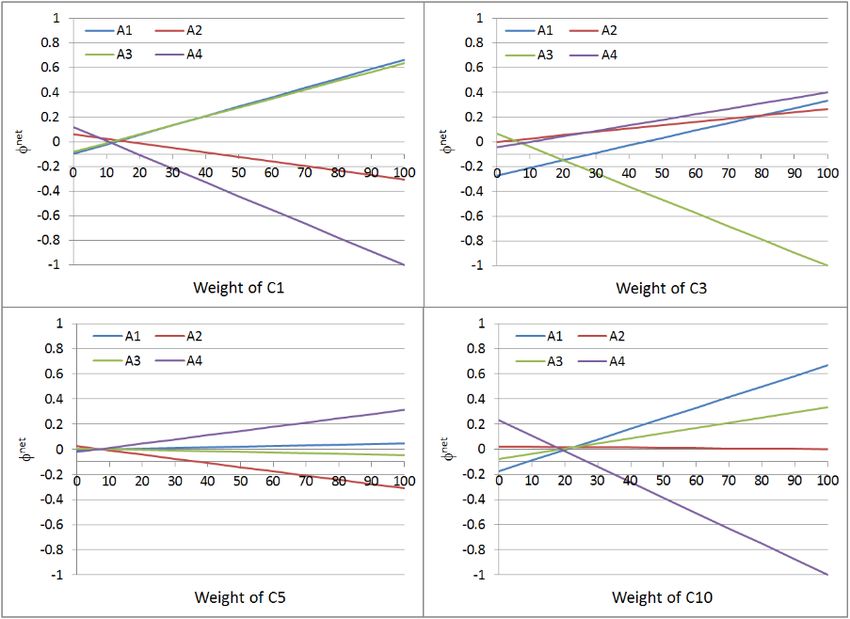
Sustainability 2016, 8, 702                                                                          7 of 22

3. Methodological Background

3.1. General Assumptions
    The adopted research procedure is based on Roy’s [52] four-stage model of a decision process.
The model consists of the following stages:

1.     determining the object of the decision and defining the set of potential decision alternatives A;
2.     analyzing consequences and developing the consistent set of criteria C;
3.     modeling comprehensive preferences and operationally aggregating performances; and
4.     the investigation and development of the recommendation, based on the results of Stage 3.

     Roy stresses that the stages do not go serially, but, for example, some elements of Stage 1
can require performing elements of Stage 2. Similarly, a decision process cannot be simplified by
eliminating individual elements of Stage 2. In Stage 3, there are three possible operational approaches
for the decision-maker in respect of the scope of aggregating performance of alternatives:

1.     use of a single synthesizing criterion;
2.     synthesis by outranking relation; and
3.     interactive local judgments with trial-and-error iterations.

      It should be noted that among methods selected to solve the decision problem, there is both
a method using a single synthesized criterion (AHP) and a method carrying out a synthesis with
the use of an outranking relation (PROMETHEE). Both of these methods are described, Sections 3.2
and 3.3, respectively.
      In Stage 1, the object of a decision is determined. The considered decision problem concerns the
selection of the best location, among those suggested, for a wind farm. The problem is considered
from an investor’s point of view, as it is the investor who wants to build a wind farm in a location with
suitable spatial, environmental, social and ecological characteristics and at the same time he or she
wants the investment to by economically rational. The decision problem is a background for presenting
a decision game, in which one alternative location is in the vicinity of Szczecin. Other alternatives
were situated in potentially the most attractive locations in other regions of the country. Assuming
a certain decision model, the decision game is to point out the conditions that the Szczecin location
would have to meet to be the best alternative. In order to accurately present all alternative locations, it
is necessary to define criteria according to which the alternative locations are to be evaluated.
      In Stage 2 of the research procedure, a set of criteria relating to individual alternatives were
assessed are prepared. The basic technical aspect depending indirectly on a location is the amount of
generated energy. It is mainly influenced by the number and power of wind turbines installed in the
wind farm. The number of wind turbines is limited by the area of the available location. It is assumed
that turbines should be at a distance of at least four times greater than the rotor diameter (usually about
80–90 m ˆ 4 m) [53]. Furthermore, the amount of generated energy is to a great extent dependent
on wind speed in a given region [54]. Therefore, among the considered criteria, the environmental
conditions, such as wind speed at the height of 100 m, were taken into account.
      Among spatial criteria, the following were taken into consideration: distance from a power grid
connection, voltage of the power grid at the connection and its vicinity, and distance from the road
network. The distance from a power grid connection influences the ease of connecting the wind farm to
the grid, whereas the voltage of the transmission grid to which the wind farm is going to be connected
is related to the voltage sweep, which consequently leads to power grid failures. Connecting high
electric power (from several dozen megawatts) wind farms to grids with too low voltage (i.e., 110 kV)
may cause damages to transmission lines or transformers [55]. The distance from the road network is
closely related to, among other things, the construction of the wind farm, since the shorter the distance
from roads, the easier it is to deliver elements on the construction site and the less expensive it is to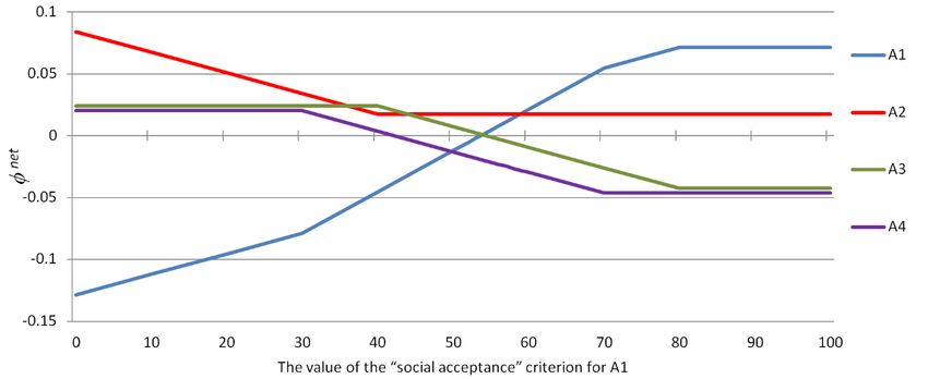
Sustainability 2016, 8, 702                                                                                       8 of 22

connect the area to the road network. It is a significant factor, for in Poland the road infrastructure in
areas characterized by good wind conditions is usually insufficiently developed [54].
     As far as ecological criteria are concerned, it is important to know if a location belongs to Natura
2000 nature protected areas. In these areas, it is forbidden to take any action that would negatively
influence the protection aims of the Natura 2000 area. However, in the case of an important public
interest, business activity permits can be issued even if this activity might have a significant negative
impact on the aims of protecting the Natura 2000 area [56]. Nevertheless, it is necessary to take efforts,
incur financial costs and devote much time to obtain such permits. Furthermore, wind farms, like
other buildings and technical facilities, cannot be located in national parks, landscape parks or nature
reserves [56].
     The most essential social factor conditioning the construction of a wind farm is social acceptance
of such an investment. This social acceptance also contains other social factors influencing the level
of acceptance, such as changes to the surrounding area, generated noise or benefits for the local
community. It is worth noting that, according to research, a high level of acceptance for a wind farm is
declared by about 12% of Poles, 85% of Poles accepts wind energy at a medium level, and 3% at a low
level [57].
     With reference to economic rationality, the basic criterion should be the investment cost, which
mainly consists of: the costs of purchase and assembly of the wind farm (turbine and tower), power grid
connection, foundations and design preparation. It is estimated that an average cost of constructing
wind farms per 1 MW of installed power amounted to PLN 6.6 million/1 MW and the price is similar to
the price of constructing an equivalent coal power station. Only gas energy requires lower investment
costs [31]. In addition, operational costs, both fixed and variable costs, should be considered. Fixed
costs include: operation and overhaul, maintenance, land lease, management, insurance, energy
consumption of the wind farm, taxes and payment to the local community. Variable costs include
variable maintenance and balance costs. In total, it is assumed that operational costs of a wind farm
in 2011 amounted to PLN 83/MWh [31]. The profit is the price for generated energy that is sold to
consumers. The average price of electric energy on the competitive market in the third quarter of 2015
came to about PLN 173/MWh [58]. However, new regulation in the form of a so-called RES auction
influences the estimated profits. The regulation reads that RES-based power stations can participate in
energy sales auctions. The bidder offering the lowest energy price will have a guaranteed purchase
price of their energy for a period of 15 years at their offered price indexed by an inflation level [59].
The reference price for an RES auction in 2016 for on-shore wind energy of the total power greater than
1 MW amounts to PLN 385/MWh [60].
     The selection of criteria used for considering location alternatives results from the fact that the
problem of location selection was considered from an investor’s point of view. Based on the above
considerations, a set of criteria is presented in Table 5.

                              Table 5. Criteria adopted for evaluation of wind farm locations.

                                    Criterion                                    Unit            Preference Direction
   C1        yearly amount of energy generated                                  (MWh)                   Max
   C2        average wind speed at the height of 100 m                           (m/s)                  Max
   C3        distance from power grid connection                                  (km)                  Min
   C4        power grid voltage on the site of connection and its vicinity        (kV)                  Max
   C5        distance from the road network                                       (km)                  Min
   C6        location in Natura 2000 protected area                               [0;1]                 Min
   C7        social acceptance                                                     (%)                  Max
   C8        investment cost                                                     (PLN)                  Min
   C9        operational costs per year                                          (PLN)                  Min
   C10       profits from generated energy per year                              (PLN)                  Max
Sustainability 2016, 8, 702 9 of 22
Locations of individual decision alternatives are presented on maps in Figure 1, against the
background of wind conditions (Figure 1a), the road network (Figure 1b), the power grid (Figure 1c),
and Natura2016,
Sustainability 2000 protected areas (Figure 1d).
8, 702 9 of 22
(a) (b)
(c) (d)
Figure 1. (a) Alternative locations on the map of wind conditions [61]; (b) Alternative locations on the
Figure 1. (a) Alternative locations on the map of wind conditions [61]; (b) Alternative locations on the
map of Poland’s
map of Poland’s road
roadnetwork
network[62];
[62];(c)(c)Alternative
Alternativelocations
locations
onon
thethe
mapmap of the
of the power
power gridgrid
[63];[63];
and
and (d) Alternative
(d) Alternative locations
locations onmap
on the the map of Natura
of Natura 20002000 protected
protected areasareas
[64]. [64].
Criteria values of individual alternatives in the spatial scope (among other things, distance from
Criteria values of individual alternatives in the spatial scope (among other things, distance from
the road network) were obtained from Google Maps. Mean wind speed was received on the basis of
the road network) were obtained from Google Maps. Mean wind speed was received on the basis of
analyses conducted by the authors of Global Atlas of Renewable Energy [65]. As far as the kind of
analyses conducted by the authors of Global Atlas of Renewable Energy [65]. As far as the kind of wind
wind turbines is concerned, research indicated that Vestas V90 3 MW (Vestas Wind Systems A/S,
turbines is concerned, research indicated that Vestas V90 3 MW (Vestas Wind Systems A/S, Aarhus,
Aarhus, Denmark) turbines would be installed in the wind farms [66]. The amount of generated
Denmark) turbines would be installed in the wind farms [66]. The amount of generated energy was
energy was calculated by means of the power output of the turbine and mean wind speed. Costs and
calculated by means of the power output of the turbine and mean wind speed. Costs and profits were
profits were calculated on the basis of the data presented in this paper concerning approximate wind
calculated on the basis of the data presented in this paper concerning approximate wind investment
investment costs and estimated energy prices. Moreover, an average value of social acceptance was
costs and estimated energy prices. Moreover, an average value of social acceptance was assumed for
assumed for the alternatives. The exception here is alternative A2, because recently Pomeranian
the alternatives. The exception here is alternative A2, because recently Pomeranian Province residents
Province residents have expressed opposition to constructing more wind farms [67,68]. Criteria
have expressed opposition to constructing more wind farms [67,68]. Criteria values of individual
values of individual alternatives are presented in Table 6.
alternatives are presented in Table 6.
Having a defined set of criteria and alternative values, Stages 3 and 4 of the decision process
were carried out; that is, preference modeling and aggregating performances as well as issuing a
recommendation. The stages were conducted separately for methods AHP and PROMETHEE.Sustainability 2016, 8, 702 10 of 22
Table 6. Criteria values for individual alternatives.
A1
Basic Data A2 A3 A4
(Szczecin)
No of turbines V90-3 MW (pieces) 23 17 21 14
Sustainability 2016, 8, 702 10 of 22
Installed power (MW) 69 51 63 42
Criterion
Table 6. Criteria values for individual alternatives.
C1 yearly amount of energy generated (MWh) 106,780 86,370 104,850 46,600
C2 average wind speed at the height of 100 m (m/s) A1
6.75 7.12 6.95 6.04
Basic Data A2 A3 A4
C3 distance from power grid connection (km) (Szczecin)
2 3 60 1
C4 power gridNo voltage on the V90-3
of turbines site of MW
connection
(pieces)and its vicinity (kV) 220
23 400
17 220
21 220
14
C5 distance from
Installed the road
power (MW)network (km) 6
69 10
51 7
63 423
C6 location in Natura 2000 protected area [0;1] 1 0 1 0
Criterion
C7 social acceptance (%) 52 20 60 50
C1
C8 yearly amount of energy
investment generated
cost (million PLN)(MWh) 106,780
455.5 86,370
336.5 104,850
416 46,600
277
C2
C9 average wind speed
operational costsatper
theyear
height of 100
(million m (m/s)
PLN) 6.75
8.9 7.12
7.2 6.95
8.7 6.04
3.9
C3
C10 distance
profits from power
from generated gridper
energy connection (km)PLN)
year (million 2
36.8 3
29.8 60
36.2 116
C4 power grid voltage on the site of connection and its vicinity (kV) 220 400 220 220
C5 distance from the road network (km) 6 10 7 3
C6
Having a defined set of criteria and alternative values, Stages1 3 and 4 of
location in Natura 2000 protected area [0;1] 0
the decision
1
process
0
wereC7carried out; that is, preference
social acceptancemodeling
(%) and aggregating performances
52 20 as well60 as issuing
50 a
recommendation.
C8 The stages
investmentwerecostconducted
(million PLN) separately for methods 455.5AHP and
336.5PROMETHEE.
416 277
C9 operational costs per year (million PLN) 8.9 7.2 8.7 3.9
3.2.C10 profits
The Analytic from generated
Hierarchy Processenergy
(AHP) perMethod
year (million PLN) 36.8 29.8 36.2 16
3.2.The
TheAHP is a Hierarchy
Analytic MCDA method
Process stemming from the expected utility hypothesis. One can distinguish
(AHP) Method
four steps:
The AHP is a MCDA method stemming from the expected utility hypothesis. One can
1. distinguish
definingfour
a decision
steps: problem and the kind of knowledge one is looking for;
2. preparing a hierarchical structure containing the main goal, intermediate goals (criteria)
1. defining a decision problem and the kind of knowledge one is looking for;
and alternatives;
2. preparing a hierarchical structure containing the main goal, intermediate goals (criteria)
3. a and
pairwise comparison of alternatives in relation to each of the criteria and a pairwise comparison
alternatives;
of importance of individual
3. a pairwise comparison of criteria; and in relation to each of the criteria and a pairwise
alternatives
4. using vectorsofof
comparison prioritiesofobtained
importance individualincriteria;
comparisons
and to receive a solution to the decision
problem [69].
4. using vectors of priorities obtained in comparisons to receive a solution to the decision problem [69].
AA decision
decisionproblem
problem and
andthethe
construction
constructionof hierarchical
of hierarchicalstructure areare
structure closely related
closely to each
related other.
to each
The decision
other. problem,problem,
The decision while constructing the hierarchical
while constructing structure,
the hierarchical is decomposed
structure, into subgoals
is decomposed into
(criteria),
subgoalswhich are placed
(criteria), which on
aresubsequent structure levels.
placed on subsequent Decision
structure alternatives
levels. play the roleplay
Decision alternatives of leaves
the
inrole
the of
structure.
leaves in One should individually
the structure. define the goals
One should individually defineofthe
thegoals
decision,
of theits subgoals,
decision, evaluation
its subgoals,
evaluation
criteria criteria subcriteria
and potential and potential subcriteria
as well as wellconnections
as hierarchical as hierarchical
between connections between
them, decision them,
alternatives
decision
and actors alternatives and actors
[70]. An example of a [70]. An example
hierarchical of a hierarchical
structure is illustratedstructure
in Figure is illustrated
2. in Figure 2.
Figure2.2.Hierarchical
Figure Hierarchical structure
structure in
in the
the analytic
analytic hierarch
hierarchprocess
process(AHP)
(AHP)method.
method.
Comparison of criteria and their alternatives comparisons are conducted with the use of a
pairwise comparison matrix. Each matrix should be reciprocal and positive. The proportion means
that every matrix element fulfills the characteristics defined by Equation (1):
aji = 1/aij (1)Sustainability 2016, 8, 702 11 of 22
Comparison of criteria and their alternatives comparisons are conducted with the use of a pairwise
comparison matrix. Each matrix should be reciprocal and positive. The proportion means that every
matrix element fulfills the characteristics defined by Equation (1):
aji “ 1{aij (1)
The interpretation of Equation (1) is as follows: if an element aij contains a value a, then the
element aji should contain an opposite value, i.e., 1/a. Moreover, elements on the main diagonal aii
should include unitary values [71]. When specifying the positivity of matrices, one needs to point out
that it should contain the Saaty’s ratio scale, i.e., from the range of 1 to 9 and their opposite values,
where 1 indicates equality of compared alternatives or criteria and 9 indicates an extreme advantage
of an alternative or criterion i over j [69]. Therefore, each matrix is completed with one of 17 values:
1/9, 1/8, . . . , 1/2, 1, 2, . . . , 8, 9 [72]. The meanings of individual values of the Saaty’s ratio scale are
presented in Table 7.
Table 7. Numerical and verbal values of the scale for the AHP method [73].
Numerical
Verbal Evaluation
Evaluation
1 Compared objects (decision alternatives or criteria) are equivalent
The decision-maker hesitates between an equivalent and weak advantage of one object
2
compared to over the other
3 A weak advantage of one object over the other
The decision-maker hesitates between a weak advantage and a considerable advantage of
4
one object compared to the other
5 A considerable advantage of one object over the other
The decision-maker hesitates between a considerable advantage and a significantly bigger
6
advantage of one object compared to the other one
7 A significantly bigger advantage of one object over the other
The decision-maker hesitates between a significantly bigger advantage and a huge
8
advantage of one object compared to the the other
9 A huge advantage of one object over the other
For every pairwise comparison matrix, a preference vector w = [w1 , w2 , . . . , wn ]T is defined,
which demonstrates the force of alternatives or criteria compared in matrices. Components of the
vector are included in the pairwise comparison matrix, which is presented in Equation (2) [70]:
In the AHP method, one calls for determining a preference vector W by determining a right
eigenvector of a matrix [74]. It is calculated by solving Equation (3):
A w “ λmax w (3)
If a pairwise comparison matrix is consistent, then there is only one non-zero eigenvalue λmax of
a matrix and it is equal to the size of the matrix. A vector w is a preference vector related to the value
λmax [61]. When there are relatively insignificant inconsistencies in the matrix, the preference vector
is one related to the highest eigenvalue (other λs have values close to 0). In other words, when the
matrix is consistent, the preference vector w corresponds to a true preference vector v. Consistency
of the matrix takes place if: aij ˆ ajk = aik for each i, j, k [75], when elements of the preference vector
are their own multiples (e.g., [1 3 6]T or [4 2 1 8]T ). Therefore, preference consistency is identical to
transitivity of evaluations, for instance, if in the decision-maker’s opinion that an alternative ai is
two times better than an alternative aj and four times better than ak , then the alternative aj should
be two times better than the alternative ak . However, the true preference vector v mostly does notSustainability 2016, 8, 702 12 of 22
contain single and exclusive values, which are their mutual multiples; therefore, the vector w is only
its approximation [76]. The phenomenon brings about the occurrence of minor inconsistencies in the
pairwise comparison matrix, which results from rounding of true preferences to the values from a set
{1/9, 1/8, . . . , 1, . . . , 8, 9}. More significant inconsistencies in the pairwise comparison matrix are most
often caused by the decision-maker’s mistakes which lie in the omission of the rule of full transitivity
of evaluations between compared alternatives [77].
Inconsistencies of a pairwise comparison matrix can be calculated by, among other things,
determining a consistency index (CI), and then by determining a consistency ratio (CR) in accordance
with Equations (4) and (5) [70]:
CI “ pλmax ´ nq{pn ´ 1q (4)
CR “ CI{R (5)
Here, R is a constant whose value depends on the size of a pairwise comparison matrix. The
values of R, dependent on the size of a matrix, are presented in Table 8.
Table 8. Values of a consistency factor R depending on the size of a matrix [78].
n 1 2 3 4 5 6 7 8 9 10
R 0 0 0.52 0.89 1.11 1.25 1.35 1.40 1.45 1.49
Solving the decision problem is obtained by a synthesis of weights of criteria and alternative
preference with relation to every criterion. This synthesis is in the form of a weighted mean in which
every alternative product of weights of criteria and evaluations of a given alternative with relation to
these criteria are added up. As a result, a generalized utility measure of this alternative is obtained. It
is presented in Equation (6) [70]:
ÿn
Ui “ wk ˚uik (6)
k=1
where Ui is the total utility of the i-th alternative, wk is the weight of the k-th criterion, and uik is the
value of the i-th alternative with regard to the k-th criterion.
3.3. The PROMETHEE Method
The PROMETHEE method uses an outranking relation in order to choose the best decision
alternative [79]. The method employs positive and negative preference flows determining how much a
given alternative outranks other ones and how much it is outranked by other alternatives [80]. The
procedure PROMETHEE I consists of four steps and PROMETHEE II consists of five steps:
1. pairwise comparison decision alternatives with regard to subsequent decision criteria;
2. applying a preference function selected for each criterion;
3. determining an alternative preference index according to accepted weights of criteria;
4. determining positive and negative preference flows for alternatives; and
5. determining net preference flow [81].
In the PROMETHEE method, the decision-maker may choose from six preference functions using
a usual criterion, a quasi-criterion with an indifference threshold, a criterion with linear preference and
a preference threshold, a level-criterion with indifference and preference thresholds, a criterion with
linear preference and an indifference area, or, finally, a Gaussian criterion, described by [82]. Preference
functions of the PROMETHEE method are graphically presented in Figure 3.Sustainability 2016, 8, 702 13 of 22
Sustainability 2016, 8, 702 13 of 22
Figure
Figure 3. Preference
3. Preference functions
functions usedininthe
used thepreference
preference ranking
rankingorganization
organizationmethod for enrichment
method for enrichment
evaluation (PROMETHEE) method [83].
evaluation (PROMETHEE) method [83].
A preference index of alternatives calculated according to Equation (7):
A preference index of alternatives calculated according to Equation (7):
n
n wk *fk (ai ,bj )
π(ai ,bjř )= w
k=1
k ˚fnk pai , bj q (7)
πpai , bj q “ k“1
n
wk (7)
ř k=1
wk
where k means a concordance factor for a pair of alternatives
k “1 compared with regard to a criterion
k in accordance with the assumed preference function. Positive and negative preference flows are
where φk means a concordance factor for a pair of alternatives compared with regard to a criterion
calculated with the use of Equations (8) and (9).
k in accordance with the assumed preference function. Positive and negative preference flows are
n
calculated with the use of Equations (8) andφ(9). +
(a )= π(a ,b )
i i j (8)
j=1
n
ÿ
φ` pa-i q “ n πpai , bj q (8)
φ (a i )=j
“1 π(b j ,a i ) (9)
j=1
Up to this point, operations in the PROMETHEE n
ÿ I and II methods are the same. While solving
´
φ pa i
the task, the decision-maker can create a partial q “ πpbj , ai q I) or total (PROMETHEE II) ranking (9)
(PROMETHEE
of alternatives. The partial ranking employed inj“the 1
method PROMETHEE I is based on isolated
Up to this point, operations in the PROMETHEE Ione
positive and negative preference flows. In the ranking, andcan distinguish
II methods indifference,
are the same. preference
While solving
and incomparability relations:
the task, the decision-maker can create a partial (PROMETHEE I) or total (PROMETHEE II) ranking
of alternatives.
The partial
an alternative ranking
ai is preferred employed
over bj (ai P bj) in theφmethod
when PROMETHEE
+(ai) ≥ φ+(b I is
j) and φ−(ai) ≤ φ−(b based
j), but on one
at least isolated
of the
positive and inequalities
negative should be
preference strongIn(>the
flows. or or φ(bj); and
be calculated:
an alternative ai is indifferent to an alternative bj (ai I bj), when φ(ai) > φ(bj) [84].
φpai q “ φ` pai q ´ φ´ pai q (10)
4. Research Results
In this method, indifference and preference relations can be distinguished:
‚ an alternative ai is preferred over bj (ai P bj ), when φ(ai ) > φ(bj ); and
‚ an alternative ai is indifferent to an alternative bj (ai I bj ), when φ(ai ) > φ(bj ) [84].Sustainability 2016, 8, 702 14 of 22
4. Research Results
Preference modeling in the PROMETHEE method consists of defining a preference direction for
each criterion (max, min), indicating preference functions used for individual criteria (usual criterion,
quasi-criterion, criterion with linear preference, level-criterion, a criterion with linear preference and
indifference area or Gaussian criterion) and determining potential thresholds and providing their
weights of criteria. These preferences are depicted in Table 9.
Table 9. Preference model for the PROMETHEE method.
Weight of Preference Preference Indifference Preference
Criterion
Criterion Direction Function 1 Threshold (q) Threshold (p)
yearly amount of energy
C1 12 max (5) 2000 20,000
generated (MWh)
average wind speed at the height
C2 8 max (3) - 1
of 100 m (m/s)
distance from power grid
C3 6 min (3) - 15
connection (km)
power grid voltage on the site of
C4 6 max (4) 0 2
connection and its vicinity (kV)
a distance from the road
C5 2 min (3) - 15
network (km)
location in Natura 2000 protected
C6 6 min (1) - -
area [0;1]
C7 social acceptance (%) 10 max (3) - 20
C8 investment cost (million PLN) 10 min (5) 1 40
operational costs per year
C9 20 min (5) 0.1 2
(million PLN)
profits from generated energy
C10 20 max (5) 0.5 10
per year (million PLN)
1 (1)—usual criterion; (2)—quasi-criterion; (3)—criterion with linear preference; (4)—level-criterion;
(5)—criterion with linear preference and indifference area; and (6)—Gaussian criterion.
Next, performance aggregation of alternatives based on the PROMETHEE procedure was
conducted. The obtained positive, negative and net values of preference flows are presented in
Table 10.
Table 10. The values of φnet and positions in the ranking of individual alternatives.
Alternative Œ+ Œ´ Œnet Rank
A1 (Szczecin) 0.2925 0.2979 ´0.0054 3
A2 0.3711 0.3535 0.0176 1
A3 0.3209 0.3168 0.0041 2
A4 0.4036 0.4199 ´0.0163 4
The analysis of the obtained ranking (Table 10) indicates that the location of Szczecin is not an
alternative that should be selected. Therefore, which actions should be taken in the active decision
model so that alternative A1 would win the first place in the ranking should be considered. There are
two kinds of action that can be taken:
1. persuading the investor to change their criteria preferences and support Szczecin as better than
Alternatives A2 and A3; or
2. taking action in order to increase the values of alternative A1 to improve the criteria that currently
the location of Szczecin is considered worse than alternatives A2 and A3.
The research, conducted with the use of a sensitivity analysis into an investor’s criteria preference
changes was carried out in such a way it could influence the improvement of the Szczecin location.
Location A1 outperforms the best alternatives with regard to criteria C1, C3, C5 and C10. Therefore, it
can be in first place in the case of increasing weights of only these criteria. The sensitivity analysis for
the weights of the above-mentioned criteria is presented in Figure 4.Sustainability 2016, 8, 702 15 of 22
Figure 4. Sensitivity analysis (criteria C1, C3, C5 and C10).
The sensitivity analysis points out that for any increase in the weights of the criteria C3 and C5,
alternative A1 will never be first in the ranking. The effect can be achieved only by increasing the
weights of the criteria C1 and C10 and proportionally decreasing the other criteria. For C1, the limit
weight when alternative A1 is first in the ranking is 35%. With reference to the initial weight of 12%, it
would be a considerable change in the decision-maker’s preference. However, for criterion C10 it is
23%, which is only 3% higher than the initial weight of this criterion. The values of φnet and rankings
obtained for the indicated weights of the criteria C1 and C10 are depicted in Table 11.
Table 11. The values φnet and positions in the ranking of alternatives for given weights of the criteria
C1 and C10.
Criterion C1—Weight: 35% Criterion C10—Weight: 23%
Alternative
φnet Rank φnet Rank
A1 (Szczecin) 0.1703 1 0.0198 1
A2 ´0.0668 3 0.0169 2
A3 0.1699 2 0.0164 3
A4 ´0.2734 4 ´0.0532 4
It is doubtful that the decision-maker changes their criteria preferences, so one needs to consider
how alternative A1 could become more attractive than A2 and A3. Considering criteria, one should
eliminate those which would be difficult to influence. These include mean wind speed, the amount of
generated energy, the distance from the road network and being situated in the Natura 2000 protected
area. Similarly, one cannot significantly influence the estimated investment costs and profits because
they are based on approximate data. One can take into account the connection of the potential wind
farm to a 400 kV power grid, which would improve the evaluations of alternative A1 with reference toSustainability 2016, 8, 702 16 of 22
the “power grid voltage” criterion. However, such action results in a significant increase in the distance
to the connection and moves the location of Szczecin into the second position in the ranking, just
behind alternative A2. Justified action would be to increase acceptance for the potential investment in
the local community (social acceptance). Indeed, an analysis of the value of this criterion for alternative
A1 without introducing any modifications to other criteria indicates that when social acceptance for
locating a wind farm in the vicinity of Szczecin is at the level of 59%, alternative A1 is ranked first. The
analysis is presented in Figure 5.
Figure 5. Analysis of the influence of the value of “social acceptance” criterion for alternative A1 on
positions in the ranking of alternatives.
It should be noted that when the value of social acceptance for alternative A1 is at the level of
ca. 40%, there is a change in the sequence of alternatives A2 and A3 in the ranking, although these
alternatives have not been modified in any way. Nevertheless, such a phenomenon is possible in the
case of methods based on an outranking relation, and PROMETHEE method belongs to this family.
In the case of the AHP method, preference modeling is carried out by pairwise comparisons
of criteria. The weights of the criteria are very close to those used in the PROMETHEE method.
A pairwise comparison matrix of the criteria is depicted in Table 12.
Table 12. Pairwise comparison matrix of criteria.
CR = 0.006 C1 C2 C3 C4 C5 C6 C7 C8 C9 C10 Vector of Weights
C1 1 2 2 2 6 2 1 1 1/2 1/2 0.1165
C2 1/2 1 1 1 4 1 1 1 1/2 1/2 0.0804
C3 1/2 1 1 1 3 1 1/2 1/2 1/3 1/3 0.0614
C4 1/2 1 1 1 3 1 1/2 1/2 1/3 1/3 0.0614
C5 1/6 1/4 1/3 1/3 1 1/3 1/5 1/5 1/9 1/9 0.0205
C6 1/2 1 1 1 3 1 1/2 1/2 1/3 1/3 0.0614
C7 1 1 2 2 5 2 1 1 1/2 1/2 0.1064
C8 1 1 2 2 5 2 1 1 1/2 1/2 0.1064
C9 2 2 3 3 9 3 2 2 1 1 0.1926
C10 2 2 3 3 9 3 1 2 2 1 1 0.1926
The performance aggregation of the alternatives was conducted by pairwise comparison of the
alternatives with regard to subsequent criteria. Aggregated preference vectors for individual criteria
as well as the final preference vector, synthesized to a single criterion, are presented in Table 13.Sustainability 2016, 8, 702 17 of 22
Table 13. Preference vectors for subsequent criteria.
CR A1 (Szczecin) A2 A3 A4
C1 0.0302 0.4269 0.1067 0.4269 0.0394
C2 0.0227 0.1576 0.516 0.284 0.0423
C3 0 0.3214 0.3214 0.0357 0.3214
C4 0 0.1667 0.5 0.1667 0.1667
C5 0.0039 0.227 0.1223 0.227 0.4236
C6 0 0.0833 0.4167 0.0833 0.4167
C7 0.0092 0.2525 0.0405 0.4545 0.2525
C8 0.0116 0.0954 0.2772 0.1601 0.4673
C9 0.0011 0.0924 0.1922 0.0924 0.6229
C10 0.0302 0.4269 0.1067 0.4269 0.0394
Preference vector - 0.2393 0.2239 0.2603 0.2765
Rank - 3 4 2 1
When comparing Tables 10 and 13, it can be easily noticed that due to the application of the AHP
method, alternatives A2 and A4 changed their positions in the ranking. The change is drastic, since the
positions were not neighboring ones, but the first and the second positions in the ranking. Moreover,
alternative A1, as in the PROMETHEE ranking, comes third.
In the case of the AHP ranking, an increase in weight of selected criteria cannot put alternative
A1 first in the ranking. This statement results from the analysis of Table 12, where it can be noticed
that there is no criterion with regard to which alternative A1 would outperform alternatives A3 and
A4, which take the leading positions in the ranking. This is why, in this case, the sensitivity analysis
was omitted.
In the next step of the research, when the preference vector of variants was calculated, similar
to the ranking obtained by means of the PROMETHEE method, whether leveling evaluations of A1
and A4 with regard to criterion C7 (social acceptance) would allow alternative A1 to be the best in the
ranking was tested. However, it turned out that it was unsuccessful, since after this, alternative A1
came second, just behind A4. Only a considerable increase in the value A1 for criterion C7 allowed it
to move to the first position and become a preferred alternative. Pairwise comparison matrices and
preference vectors for social acceptance and the final ranking of alternatives, obtained with a given
pairwise comparison matrix, are presented in Tables 14–16.
Table 14. Pairwise comparison matrix for a criterion “social acceptance” and the final ranking
of alternatives.
CR = 0.0092 A1 A2 A3 A4 Preference Vector C7 Final Preference Vector Rank
A1 1 7 1/2 1 0.2525 0.2393 3
A2 1/7 1 1/9 1/7 0.0405 0.2239 4
A3 2 9 1 2 0.4545 0.2603 2
A4 1 7 1/2 1 0.2525 0.2765 1
Table 15. Modified pairwise comparison matrix for a criterion “social acceptance” and the final ranking
of alternatives.
CR = 0.0092 A1 A2 A3 A4 Preference Vector C7 Final Preference Vector Rank
A1 1 9 1 2 0.3756 0.2524 2
A2 1/9 1 1/9 1/7 0.0376 0.2236 4
A3 1 9 1 2 0.3756 0.2519 3
A4 1/2 7 1/2 1 0.2112 0.2721 1You can also read