House-tile takeover? The effects of home-sharing on the Amsterdam housing market
←
→
Page content transcription
If your browser does not render page correctly, please read the page content below
House-tile takeover? The effects of home-sharing on the
                Amsterdam housing market
                                    Lund University,
                                       Team 5

                                      April 9, 2021

Abstract
     We study the effect of AirBnB on housing prices in Amsterdam, using several
econometric approaches to show that these effects have a causal interpretation. These
include i) a hedonic regression model, incorporating a double-lasso procedure to select
control variables, ii) a fixed effects model which exploits within-address and across-
sale variation in AirBnB proliferation for a subset of properties which are sold multiple
times and iii) an instrumental variables shift-share approach, merging external data
from TripAdvisor.com, exploiting the fact that the interaction between the location
of tourist amenities and Google searches exogenously predicts the spread of AirBnB
listings. Across these specifications, we find a positive and significant effect of AirBnB
listings on prices. Specifically, we find that an increase of 100 AirBnB listings within
250 metres of a property causes the price of that property to increase by between 5
and 12%. Furthermore, we identify evidence of non-linear and heterogeneous effects.
In a broader market equilibrium analysis, we identify that the increase in house prices
is driven by an increase in asking prices. Furthermore, using an instrumental variables
approach to incorporate the causal effect of asking prices into our model, we find that
asking prices and AirBnB density affect sales prices simultaneously, while we find no
effects on sales volume or time on the market.

                                            1
Contents
1 Introduction 3
2 Theoretical Context 4
3 Data 6
4 Reduced Form Effects on House Prices 7
4.1 Hedonic Regression . . . . . . . . . . . . . . . . . . . . . . . . . . . . . . . 7
4.1.1 Method . . . . . . . . . . . . . . . . . . . . . . . . . . . . . . . . . . 7
4.1.2 Results . . . . . . . . . . . . . . . . . . . . . . . . . . . . . . . . . . 8
4.2 Address Fixed Effects . . . . . . . . . . . . . . . . . . . . . . . . . . . . . . 9
4.2.1 Method . . . . . . . . . . . . . . . . . . . . . . . . . . . . . . . . . . 9
4.2.2 Results . . . . . . . . . . . . . . . . . . . . . . . . . . . . . . . . . . 9
4.3 Shift-Share Instrument . . . . . . . . . . . . . . . . . . . . . . . . . . . . . 10
4.3.1 Method . . . . . . . . . . . . . . . . . . . . . . . . . . . . . . . . . . 10
4.3.2 Results . . . . . . . . . . . . . . . . . . . . . . . . . . . . . . . . . . 11
4.3.3 Heterogeneity . . . . . . . . . . . . . . . . . . . . . . . . . . . . . . 12
5 Market Equilibrium Analysis 13
5.1 Transaction volumes . . . . . . . . . . . . . . . . . . . . . . . . . . . . . . 13
5.2 Asking prices, sales prices and time on the market . . . . . . . . . . . . 13
5.2.1 Method . . . . . . . . . . . . . . . . . . . . . . . . . . . . . . . . . . 13
5.2.2 Results . . . . . . . . . . . . . . . . . . . . . . . . . . . . . . . . . . 14
6 Conclusion and Discussion 15
7 Tables and Figures 19
Appendix A 25
21. Introduction
The price of houses in Amsterdam has increased exponentially in recent years. The
rapid growth of AirBnB, a platform that allows individuals to rent out their homes
on a short-term basis, has coincided with this dramatic increase. This has lead policy-
makers to wonder whether home-sharing business models have been partly to blame
for the explosion in prices.
Identifying the causal effect of AirBnB proliferation on house prices is difficult. First,
it is possible that some unobserved characteristics of homes could be correlated with
increased AirBnB proliferation. For example, demand for homes in more gentrified
areas could be correlated with increased AirBnB lettings. This would make it difficult
to separate the two factors and identify the causal effect of AirBnB. Second, we have a
selection issue in that the locations that AirBnBs establish themselves are likely not
exogenous. AirBnBs are likely to appear in places deemed attractive to tourists, as
tourists are the main consumers of these short term rentals.
We identify the causal effect of AirBnB on residential property prices using three
identification strategies. These are: i) a hedonic regression framework, incorporating a
double-lasso procedure to select the control variables with the most predictive power
with regards to property prices and AirBnB proliferation. ii) A fixed effects model
which exploits within-address and across-sale variation in AirBnB proliferation for a
subset of properties that are sold multiple times. This approach removes any omitted
variables bias remaining in the hedonic model. iii) An instrumental variables shift-
share approach, merging external data from TripAdvisor.com on tourist amenities
and Google search trends, exploiting the fact that the interaction between the location
of tourist amenities and Google searches exogenously predicts the spread of AirBnB
listings. This approach serves to remove any biases caused by the selective locations of
AirBnB listings. Furthermore, in a broader market equilibrium analysis, we investigate
the relationship between AirBnB, asking prices, time on the market and final sales
prices. Adopting a further instrumental variables approach, we identify the causal
effect of asking price on time on the market and final sales price.
We find significant effects of AirBnB proliferation on house prices in Amsterdam.
The effect sizes are of a similar magnitude across all of our identification strategies,
confirming the robustness of our results. In our preferred specification, using the
instrumental shift-share approach, we estimate that an increase of 100 AirBnBs within
a radius of 250 meters of a household leads to a price increase of approximately
8%. This corresponds to an increase of e24,000 on the mean price. We investigate
heterogeneity in the effect of AirBnB by dwelling size (measured in terms of number
of rooms) and time period following the introduction of AirBnB. We find considerable
heterogeneity in the effects of size of dwelling, with the effect on dwellings of four or
more rooms being almost twice as large as the effect on dwellings with three rooms
or less (5.8% versus 10.4%). We moreover find that the effect of AirBnB density on
the price of all dwellings was relatively similar in the periods 2008-2014 and the more
recent period 2017-2018.
In our market equilibrium analysis, we find that neither asking prices nor AirBnB
3density have a significant effect on length of time on the market or sales volumes. This
suggests that the housing market in Amsterdam is efficient. We find that asking prices
are closely related to final sales prices, with a 1% increase in asking price leading to
an approximately 0.6% increase in sales price. Asking price is a stronger predictor
of final sales price than AirBnB density, but AirBnB density remains a strong and
economically significant predictor of sales price (effect size 3%) when asking price is
accounted for.
The rest of this paper proceeds as follows. In section 2 we present our theoretical
model for the effect of AirBnB density on house prices. This model then guides our
subsequent analyses. In section 3 we describe the data used. In section 4 we present
the methodology and results for our three identification strategies used to establish the
causal effect of AirBnB on house prices, and additionally investigate heterogeneity in
these effects. In section 5 we conduct a market equilibrium analysis, investigating the
effect of AirBnB density on transaction volumes and the relationship between asking
prices, sales prices and time of the market. In section 6 we conclude and discuss policy
implications of our findings.
2. Theoretical Context
To understand how short-term rentals via sharing platforms could potentially affect
house prices, we follow the model by Garcia-López et al. (2020) in which house prices
depend on owners choices to rent short- vs long-term and location choices of residents
and tourists. From the model, we will gain hypotheses that we can test empirically in
our analysis, guidance for our model selection and insights about potential threats to
our identification strategies.
In the Garcia-López et al. (2020) model, a city consists of two neighbourhoods, a
city neighbourhood which is of a fixed size C and a suburb neighbourhood s. Housing
prices depend on the choices of owners to rent their properties either short term,
receiving the annual rent, T, minus a cost, b j , or long-term, receiving an annual rent
of Qc . This choice occurs because the traditional segmentation between short-term
rentals to tourists and long-term rentals to residents diminished with the evolution of
sharing-platforms such as AirBnB. Housing prices further depend on the choice of
tourists and residents to reside in either one of the neighbourhoods.
In the market-clearing equilibrium, the share of properties that are rented short-
term b∗j is given as follows:
( A t − Ar ) + C − γ (1 − C )
b∗j = (1)
2C + (1 − α) + γ(C )
where At and Ar represent a valuation of the neighbourhood’s amenities by tourists
and residents, respectively. This implies that the share of properties that are rented
short term depends heavily on the difference between the tourists and the residents
valuation of the amenities.
Finally, following Garcia-López et al. (2020), we model housing prices as a dis-
4counted cash flow of annual rents:
∞ Z 0
c
P = ∑δ t
[(1 − b∗j ] Qc +
b
∗
j (T − b j )db j ] (2)
t =1
in which long-term rentals are obtained from inserting the market clearing condi-
tion from eq. (1) into the marginal resident’s willingness to pay function. We follow
Garcia-López et al. (2020) and model the residents willingness to pay function as
∗ ) = A − α F ( b∗ ) + e∗ + Qs , where α F ( b∗ ) reflects the negative externality aris-
Qc (eir r b j ir b j
ing from tourism and eir ∗ reflecting the residents preference to live in neighbourhood c
instead of neighbourhood s. The equilibrium price of long-term rents is thus given as
follows:
Qc = (1 − C )(1 + γ) + Ar + (C + γC − α)b∗j (3)
The predictions of eq. (1) to eq. (3) are thus that an increase in AirBnB density leads
to an increase in the supply of short term rents, coinciding with an decrease in the
supply of long-term rents. This increases the price of long-term rents, making property
investments more attractive to prospective buyers, thereby leading to increased sales
prices.
The model of the transaction processes in the housing market suggested in Dubé
and Legros (2016) allows us to predict potential mechanisms underlying this effect. In
their model, the final sales price is determined as the result of a two-step process. First,
the seller lists the asking price. In the second step, both the final sale price and the
time on the market are determined simultaneously in the negotiation process between
the seller and the buyer, which depends on the motivation of both agents. Increasing
AirBnB density in a neighbourhood constitutes a demand shock to the housing market.
In an efficient market, this demand shock will translate into increased sales prices.
Assuming sellers are rational agents, they will incorporate higher price expectations
in their listing prices, increasing asking prices to the same extent. Given that housing
supply is inelastic, this upward shift in demand will lead to increased prices but will
have a minimal effect the quantity demanded or supplied. The time on the market
will thus be unchanged.
Overall, the implications we gain from this model are as follows:
• Greater AirBnB activity in a neighbourhood increases house prices, with asking
prices increasing to the same extent. Moreover, a model of an efficient, inelastic
housing market predicts that an increase in sales prices does not significantly
affect the transaction volume of house sales or time on market.
• The model highlights that an important threat to our identification strategy is
that AirBnB activities and the willingness to pay of local residents could move
together and thereby simultaneously affect housing prices. This raises concerns
for the identification of a causal effect of AirBnB on housing prices.
• The model further predicts that AirBnB activities depend on amenities in the
neighborhood, as they are differently valued by tourists and residents.
5Testing these hypotheses empirically is challenging for at least two reasons. First,
we face the threat of omitted variable bias. Houses and neighbourhoods with different
AirBnB densities are likely to differ also with respect to other characteristics that are
correlated with house prices. For example, AirBnB density might be higher in areas
with a high degree of gentrification, for which residents have a higher willingness to
pay which leads to higher house prices. Those factors could be unobserved to the
econometrician and therefore difficult to control for. As a result, it is insufficient to
just compare houses in areas with high and low AirBnB densities.
Second, we potentially face selection bias. This is a direct implication of the above
drafted model, in which we showed that tourists and residents value local amenities
differently. Hence, AirBnB listings may be more likely to occur near the city centre,
where house prices may increase at a different trajectory to those in more suburban
areas for other reasons than the spread of AirBnB. Just comparing houses in areas
with different AirBnB densities might thus bias the estimates.
Ideally, we would like to identify the causal effect in an experimental set-up in
which AirBnB densities within 250 meters are randomly assigned to otherwise identical
houses. This would allow us to isolate the causal effect of AirBnB activity on house
prices. Such an experiment is, however, not feasible in practice as AirBnB density
cannot be randomly assigned since it is the result of numerous individual choices by
house owners and prospective tenants and tourists. Moreover, it would not be possible
to find an adequate sample of identical houses within Amsterdam that one could
assign AirBnB densities. In the remaining parts of the paper, we will discuss in detail
how to overcome these potential sources of bias and suggest different identification
strategies that allow us to estimate the causal effect of AirBnB density on house prices.
3. Data
The analysis in this paper is mainly based on one dataset provided with the case. The
data contains 108,441 observations about housing transaction prices in Amsterdam
from 2000-2018 and was made available via Brainbay. The data include the final
transaction price for each sale (in e), the asking price (in e), the time on the market
(in days), information about the year of construction, the type (Apartment, Row house,
Semi-detached house, Corner house, Two under one roof, Detached house), and the
size of the house (size (measured in m2 ), the volume (measured in m3 ), and the number
of rooms). Further, information is provided for whether a garden and/ or a parking
spot is present, if the house is listed as a monument and a score about the general state
of the quality. Additionally, we have data about the number of AirBnB listings within
250 metres of a property and the distance to the nearest AirBnB listing, also measured
in metres. We identify and set to missing outliers in the volume and number of rooms
variables, which affects 353 observations.
In table 1 we present the descriptive statistics. The average house has 3 rooms and
is around 86.667 m2 in size. Approximately 86.4% are apartments, whereas only 0.3%
are Semi-detached houses. 27.3% of the houses have a garden, while only 10% have
a parking space available. Most of the houses were built between 1906-1930 (27.9%).
6The average sale price is e301,044, while the average asking price is slightly higher
with e310,463. In Amsterdam a house spends approximately around 117 days on the
market.
In fig. 1, we illustrate the rapid growth of AirBnB listings in Amsterdam over the
last decade. As AirBnB was founded in 2008, we find a strong increase of numbers
of AirBnBs starting in 2008. At the end of 2014, AirBnB and the city of Amsterdam
signed an agreement that AirBnB would provide hosts with improved information on
the rules for home sharing and to simplify the processing of tourist taxes, making it
simpler for AirBnB hosts. As can be seen, this led to a sharp increase in the number
of listings in 2015, although this growth slowed somewhat in further years. In fig. 2
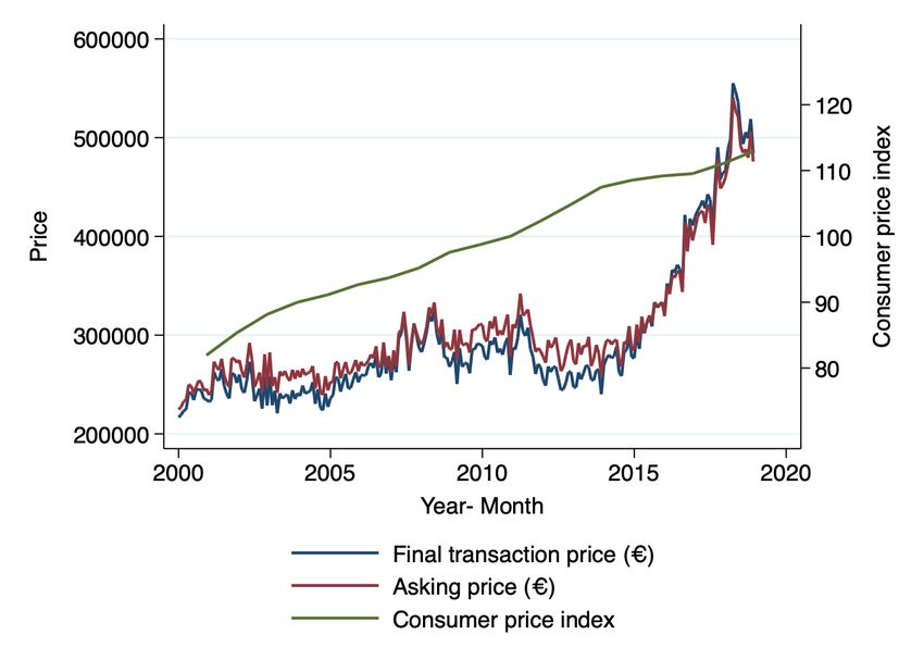
we present the development of the transaction and the asking price from 2000 to 2018.
It is evident that the existing gap between the transaction and the asking prices of
houses in Amsterdam has been decreasing in recent years, particularly from around
2015. Further, for reason of comparison we add the Consumer price index (2010=100)
our graph. Clearly, the increase in the presented house prices is steeper as for the
consumer price index in the Netherlands.
4. Reduced Form Effects on House Prices
4.1. Hedonic Regression
4.1.1. Method
Traditionally, property prices are modelled using hedonic regression models. In this
method, the price of a property is estimated as the sum of the implicit prices of its
components (Jones, 1988). Thus, in our first specification we estimate the following
model:
log( Pi ) = AirBnBi + Xi + ei (4)
where the log price of house i depends on the number of AirBnB listings within
250m of the house, a vector of house characteristics Xi and a remaining error ei . We
use the density of AirBnB listings around the property rather than the distance to the
next AirBnB listing because density represents the overall AirBnB activity around a
property which is the relevant determinant that affects house prices via an increased
share of short-term rentals relative to long-term rentals as presented in section 2. For
ease of interpretation, we divide this variable by 100.
We select the variables to include in the vector Xi using the Lasso double selection
method by Chernozhukov et al. (2015). Thereby, we perform Lasso regressions and test
whether the selected variables are predictive of either our outcome variable, log house
prices, or our treatment variable, AirBnB density. Those variables that prove to be
predictive of either the log prices or AirBnB density are included in the hedonic price
model and will also be included in all our subsequent models as control variables.
As we discuss in section 4.3.1 , we find clustering in assignment of AirBnB density at
the zip-code level. Hence, we cluster standard errors at the zip-code level in all our
specifications (Abadie et al., 2017).
7The hedonic price method is, however, sensitive to omitted variable bias (Cropper
et al., 1988). This means the estimates can be sensitive to unobserved house character-
istics that are correlated with the AirBnB density and determinants of the house price.
In addition, as we show in section 4.3.2, AirBnB density is not randomly assigned
across the city but is in fact higher in touristy areas. House prices in touristy areas are
likely to differ from house prices in other areas because of unobserved characteristics.
All observable characteristics being equal, house prices in touristy areas might be
higher because of gentrification processes (Garcia-López et al., 2020). On the other
hand, house prices could be lower in touristy areas, everything else being equal, due
to negative externalities such as noise and congestion. The estimates of the hedonic
regression model would then be biased.
For this reason, we acknowledge that the estimates from this specification should
be interpreted as descriptive rather than causal. The results from this regression
should therefore be seen as a baseline for comparisons with subsequent specification
models.
Furthermore, the hedonic regression cannot remove the issue of selection of
AirBnBs into different areas of the city. Specifically, AirBnBs listings may be more
likely to occur in areas near the city centre, as tourists generally prefer to locate
themselves as close to the centre of a city as possible. Additionally, the growth of
AirBnB occurred in parallel to the recovery from the global financial crisis. If areas of
high demand for tourists are also areas of high real estate demand in general and of
areas where demand recovered faster after the crisis, then our estimates will be biased
up since increased AirBnB density is also correlated with other demand.
4.1.2. Results
In table 2 we present our results from estimating eq. (4). In column (1), we regress the
log price against the density of AirBnBs without controls, and in column (2) and (3)
we add different sets of control variables. Across all specifications, our coefficients are
positive and highly significant. The estimate presented in column (1) indicates that
an increase of 100 AirBnB listings within 250m is associated with an increase in the
house price of 14.2%. Including different sets of control variables decreases the effect
size to 5.1% with all controls included, while including only lasso-selected controls
increases the effect size to 12.6%. The fact that the effect size increases considerably
when we only control for the lasso-selected variables indicates that including all of the
control variables in column (2) causes over-fitting, removing variation in the density
variable and biasing the results downward.
In column (4), we include the squared density of AirBnB listings to test for non-
linear effects. As the coefficient on density increases significantly and the coefficient on
the quadratic term is negative and significant, this indicates that the effect of AirBnB
listings on house prices is positive, but diminishing at higher levels of AirBnB density.
84.2. Address Fixed Effects
4.2.1. Method
As discussed above, hedonic regressions cannot truly remove the issue of omitted
variable bias. In order to address this problem, we exploit the fact that many properties
in our data are sold on multiple occasions in a fixed effects set-up. By including address
fixed effects in our model, we are able to leverage within-address, across-sale variation
in AirBnB density to identify the effect of increased saturation of AirBnB listings on
sales prices. We therefore estimate the following equation:
log( Pit ) = AirBnBit + γi + δt + Xi tβ + ei (5)
where log( Pit ) is the log sales price of address i at sale t, AirBnB represents the
number of AirBnB listings within 250 metres of an address, divided by 100 and γ and
δ are address and time fixed effects, respectively. Xi t a subset of our lasso-selected
control variables, which may change over time, and we cluster standard errors at the
4-digit postcode level.
While this approach removes any omitted variables bias at the address level, biases
may still arise due to selection in two ways. First, there may be selection in the types
of properties which are sold multiple times. For example, as will be discussed in
section 4.3.1, AirBnB density is higher in areas with more tourist amenities, which
correspond to areas in and around the city centre. If homes near the city centre are
more likely to be traded as investments, the effects of AirBnB saturation may be lower
for these homes, biasing down our estimates. To deal with this issue, we follow Miller
et al. (2019), who suggest a re-weighting procedure to adjust for selection into fixed
effects panels. Specifically, we estimate a probit model, predicting the propensity of
each address to appear in our data more than once. We estimate this propensity as a
function of our lasso-selected control variables, the price of a property’s first sale and
its year of first sale, as properties sold for the first time in more recent years have less
time to re-appear in our data.
A second source of selection bias is that it cannot remove the issue of selection
of AirBnB listings into an area, as discussed in section 4.1.1. A further downside of
this methods is that, as we identify within-address variation in AirBnB density, we
are not able to identify non-linear effects as density is de-meaned at the address-level
and non-linear effects would be identified at different levels of AirBnB density, which
would cause inconsistency in our estimates.
4.2.2. Results
The table 3 presents our results from estimating eq. (5) including different sets of
control variables. Across all specifications, the coefficient of AirBnB density is positive
and significant. In column (1), we estimate the model only including time and address
fixed effects, without any further controls. Our results indicate that an increase of 100
AirBnB listings within 250m of a house leads to an increase in the house price of 14.3%
percent. This effect size is almost identical to the effect estimated with the hedonic
regression model without controls, indicating that omitted variable bias is not a major
9concern here. Including the lasso-selected control variables, the effect size is reduced
to 5.1% percent.
To test if selection into multiple sales could be a concern, we present the results
from estimating the propensity for multiple sales in table A1. The results show that
almost all characteristics do significantly affect the probability for multiple sales. For
example, the type of the house is a predictor of multiple sales, with apartments being
more likely to be sold multiple times than other house types and more recently built
houses being less likely to be sold several times. In addition, more expensive homes
and larger homes are less likely to be sold multiple times. We present the coefficients
for the regression of eq. (5) with the corresponding re-weighted fixed-effects in column
(3) of table 3. The coefficient for AirBnB density is almost identical to the estimate in
column (2), suggesting that selection into multiple sales is not a major concern in this
case.
4.3. Shift-Share Instrument
4.3.1. Method
To tackle the endogeneity of Airbnb location, we follow Barron et al. (2021) and Garcia-
López et al. (2020) in using a shift-share instrument that combines the following:
i) cross-sectional variation in the location of tourist amenities across addresses and
ii) the aggregate time-variation in AirBnB activity. The composition of an IV, using
the combination of a potentially endogenous cross-sectional exposure variable and a
plausibly exogenous time-varying variable , was first suggested by Bartik (1991) and is
increasing in popularity. For our cross-sectional “share” component of the instrument,
we construct an index of the “touristy-ness”of an address.
Our instrument aims to capture the set of amenities that tourists appreciate while
not being of particular interest to residents. We produce a list of the Amsterdam’s
tourist amenities and collect the number of reviews of each tourist attraction, using
data from TripAdvisor.com.
To determine the measure of tourist amenities we use the following approach:
1
Tourist Amenities i = ∑ dist i,k
× Reviews k (6)
k
where k denotes the amenity, disti,k is the distance in meters between the address i
and the amenity k. Reviewsk indicates the number of of TripAdvisor Reviews.
Coming to the “shift” part of our instrument, we follow Barron et al. (2021)
and Garcia-López et al. (2020) by using worldwide searches in Google for “AirBnB
Amsterdam”. This data is normalised to a 0-100 scale, with 100 representing the month
with the highest number of searches. The variable is measured at the monthly level.
The intuition behind our used shift-share instrument is the following: the touristy-
ness of an address predicts the location of the AirBnB listings, while Google searches
for the term ‘AirBnB Amsterdam’ predicts the time period when the listings appear. In
order for our instrument to be valid, it must necessarily be uncorrelated with address-
10specific time-varying shocks to the housing market. Our instrument is only allowed to
be correlated to the transaction price through its effect on AirBnB listings. Specifically,
in areas with AirBnB listings, we should see a positive relationship between the
instrument and the transaction prices. Whereas we should not observe a positive
relationship between the instrument and the transaction prices in areas with few or no
AirBnB listings. Furthermore, we argue that our instrument is exogeneous, since it is
relatively unlikely that inhabitants’ preferences to locate close to tourist attractions
changed during the period 2000–2018 for reasons other than tourism. Barron et al.
(2021) investigate the validity of a similar instrument extensively in the context of the
United States housing market and argue that it is a valid instrument.
As such, we estimate the following system of equations:
ˆ i + ei
log( Pi ) = β AirBnB (7)
ˆ i = α + γTouristAmenitiesi ∗ Gt + ε i
AirBnB (8)
where log( Pit ) is the log sales price of property i, AirBnB represents the number of
AirBnB listings within 250 metres of an address, divided by 100. TouristAmenities
represents the touristy-ness index of a property and Gt represents the trend in google
searches for “AirBnB Amsterdam” during the month of sale t. We again cluster
standard errors at the 4-digit postcode level. While we are unable to identify non-
linear effects in an IV framework (Mogstad and Wiswall, 2010), we use this model to
identify heterogeneities in the effect of AirBnB on prices.
4.3.2. Results
In table 4 we present both first stage and reduced form results of these analyses. The
F-statistic of our instrument is 30.25, indicating that our instrument is relevant for
this analysis (Angrist and Pischke, 2008). Our first stage results indicate that the
instrument is strongly predictive (at the 1% significance level) of AirBnB density. This
implies that there does in fact exist strong selection of AirBnB listings across the city
of Amsterdam, with listings more likely to appear in more touristy areas at times
when demand is high. While this could call into the question the results presented
in section 4.1.2 and section 4.2.2 due to the presence of selection bias. However, as
the effects we identify using our shift-share instrument are similar in magnitude to
those previously identified, we believe that our identification strategies can still be
considered causal.
The reduced form results also suggest that the instrument is strongly predictive
of the log of sales price. The coefficient on the instrument in the reduced form
regression is moreover very similar to the coefficient on AirBnB density in of our
hedonic regression without controls (table 2, column 1) as well as the coefficient on
AirBnB density in our address fixed effects analysis without controls. Moving on to
our IV 2SLS results, when we do not include controls, we find that an increase of 100
AirBnB listings within a radius of 250 meters of a household increases the sale price
of that home by 29.6% percent. This estimate does not, however, include controls for
unobserved heterogeneity that is constant at the four-digit postcode level over time,
11or unobserved heterogeneity that is constant across all postcodes but changes over
time. When including calendar year-month and postcode fixed effects, our estimate is
reduced to 9.6% but remains significant at the 1 percent level. When we additionally
include controls selected by the Double-Lasso selection method, the effect remains
significant and reduces only slightly in magnitude to 0.077. This estimated effect of
7.7% is comparable to our estimates in the address fixed effects analyses with controls
(both the standard version and using the re-weighting method proposed by (Miller
et al., 2019)), though considerably smaller than the effects estimated in our hedonic
regressions when including lasso-selected covariates.
4.3.3. Heterogeneity
It is possible that the effect of AirBnB differs by house type or size, or that the effects
of AirBnB density change over time as the market becomes more saturated. We
investigate whether the effect of AirBnB on house prices differs by the number of
rooms a household has, comparing households with four or more rooms compared
to those with three or less, and between the six-year period immediately following
the entry of AirBnB compared to next four years, split into periods of two. We believe
these are interesting splits to make in the sample because the City of Amsterdam has
a rule that it is illegal to rent to more than four tenants simultaneously, potentially
making dwellings of four rooms or more less attractive as AirBnB rental properties.1
We choose our particular time period split for investigating heterogeneity for two
reasons. First, in December 2014 AirBnB and the City of Amsterdam agreed that
AirBnB would make the rules for homesharing in the city clearer and simplify the
process for the payment of tourist taxes by hosts2 . These two changes thus made it
easier for potential AirBnB hosts to start operating in the city. Second, AirBnB and the
City of Amsterdam agreed in December 2016 that AirBnB would automatically cap the
number of nights that hosts are allowed to rent out their entire homes to 60(Almagro
and Domınguez-Iino, 2019). The policy of not being allowed to rent out one’s entire
home for more than 60 nights in a calendar year had been in place previously, but
only weakly enforced. Enforcing this rule directly through the AirBnB platform made
it more difficult to get around. It is thus possible that investing in properties with the
intention of renting them on AirBnB became less attractive in the post-2017 period.
We find that the effect of AirBnB on house prices is strong and significant in the
six-year period following the entry AirnBnB to the short-term rental market (see
table 5). We estimate a very large, but non-significant effect in the second period
(2015-2016). In the third period the effect size is similar to that estimated for the first
six year period following the introduction of AirBnB, but is only significant at the
10% level. This may be a power issue considering we “only” have observations on
11,637 homes sold, multiple controls and fixed effects for both four-digit post-code
and month-year. Overall, in the first period, an increase of 100 AirBnBs within a 250
meter radius leads to an increase in house price of 23.4% percent and in the period
2017-2018 an increase in AirBnB density of the same amount leads to an increase in
1 https://www.amsterdam.nl/wonen-leefomgeving/wonen/vakantieverhuur/vergunning/
2 https://www.airbnb.es/press/news/amsterdam-and-airbnb-sign-agreement-on-home-sharing-and-tourist-tax
12house prices of 24.5% percent. The unstable result in 2015-16 is potentially due to the
dramatic readjustment in AirBnB listings observed in the period 2015-2016 (see fig. 1).
The effect of AirBnB is significantly different for dwellings with three rooms or
less compared to those with four rooms or more, with the effect size for dwellings
with four rooms or more nearly double that for dwellings with fewer rooms. This is
interesting considering the above-mentioned rule forbidding rentals to more than four
tenants simultaneously. Anecdotally, it seems, however, that this rule only became
salient to many AirBnB hosts in January 2017 3 . It is thus possible that potential hosts
invested in large properties to rent out without knowing about this regulation.
5. Market Equilibrium Analysis
There likely exist several mechanisms underlying the positive effect of AirBnB on
house sales prices identified in the previous sections. In the following sections we
take a broader look at how AirBnB has affected the market equilibrium. Specifically,
we examine the effect of AirBnB density on transaction volumes and asking prices.
Furthermore, we exploit an instrumental variables approach to incorporate the causal
effect of increased asking prices into our model, examining how AirBnB density and
asking prices simultaneously determine the time a property spends on the market and
final sales prices.
5.1. Transaction volumes
In this section we examine the question of the impact of AirBnB on the transaction
volume in the context of Amsterdam. While the model presented in section 2 does not
predict any change in sales volumes, if the market is inefficient, a demand shock may
lead to an increase in sales volumes and a shorter time on the market if it takes time
for buyers and sellers to coordinate on the equilibrium price.
As shown in table 6, when we instrument density with our shift-share instrument
and include either the required controls for time and zip codes or our lasso-selected
controls, we do not identify any significant effects of AirBnB density on transation
volume. Ultimately we find that an increase of 100 in the average density of AirBnBs in
the postcode is associated with a not economically meaningful increase in transaction
volume of only 0.09 transactions.
5.2. Asking prices, sales prices and time on the market
5.2.1. Method
In this section, we explore the effect of AirBnB density on asking prices and time
on the market, as well as its effect on the relationship between asking price, time
on the the market and the final transaction price. Identifying this relationship is
3 https://community.withairbnb.com/t5/Hosting/Some-news-on-how-Airbnb-will-now-have-to-enforce-existing/m-p/272415/highlight/true#
M64239
13methodologically challenging due to the underlying endogeneity of asking prices and
time on the market. This problem arises as each of the asking price, sales price and
time on the market depend on the motivation of both the seller and the buyer. Hence,
using any one of these variables to predict another induces an endogeneity problem as
the unobserved motivation of both the seller and the buyer is hidden in the error term.
To counteract the endogeneity issue, we exploit the fact that asking price is set by
the seller before time on market or sales price are realised. We propose an instrumental
variable approach based on the method suggested in Dubé and Legros (2016). We
instrument the asking price of a property with the mean log sales price of all properties
transacted before that property entered the market. These prior sales prices are
residualised net of our lasso-selected controls. Using this instrument, we exploit the
fact that the intertemporal relationships in the variables are unidirectional, meaning
that the previous transactions are exogenous to the individual seller at the time of
listing the asking price. This approach allows us to explore the effect of asking prices on
final transaction prices and time on the market. The key assumption here are a strong
first stage and the exclusion restriction. While we are able to test for the presence of a
strong first stage, it is more difficult to test the exclusion restriction. In our case, this
requires that previous asking prices affect contemporaneous time on market and sales
price only via contemporaneous sales price. The greatest threat to our identification
strategy is that previous sales prices in a postcode affect contemporaneous sales
prices via expectations that are not captured by contemporaneous asking prices. As
the model presented in section 2 proposes that higher sales price expectations will
be capitalised by higher asking prices, and as this is corroborated by our results in
section 5.2.1, we believe that there are no other remaining avenues through which
previous asking prices affect our outcomes.
From this relationship, it becomes evident that we cannot instrument time on the
market with time on the market in previous transactions. As contemporaneous asking
price affects contemporaneous time on the market, it is likely that past asking prices
affect past time on market, thus violating the exclusion restriction for a time on market
instrument.
In a next step, we will combine this instrumental approach with the shift-share
instrument for AirBnB density constructed in section 4.3.1 to explore how AirBnB
listings and asking prices affect other outcomes simultaneously. Doing so, we will
first explore the effect of AirBnB density on asking prices and time on the market.
Next, we will introduce the instrumented asking prices to the model to identify the
simultaneous effects of AirBnB density and asking prices on time on market and sales
prices.
5.2.2. Results
We present results for these analyses in table 7. The first stage of our instrument
for asking prices is negative and significant with an F-statistic of 324. We find that
AirBnB density has a positive and significant effect on the asking price (column 1),
and the size of this effect is very similar in magnitude to the effect of AirBnB density
on the sales price found above (replicated for convenience in column 5). In both cases,
14the effect of an increase of 100 AirBnBs within a radius of 250 meters of a property,
instrumented using our plausibly exogenous shift-share instrument, on house prices
is of approximately 8 percent. this implies that the effects on sales prices identified
in section 4 are driven by the capitalisation of higher expectations in higher asking
prices.
Looking to time on the market, we do not find any significant or economically
meaningful effects of either AirBnB density or asking prices on time on the market (in
days)4 .
Finally, in examining final sales prices once more. we find significant and positive
effects of asking prices on final sales prices. When asking price is included alone in
the model as a predictor of sales price, we fine that a 1% increase in asking prices
leads to a 0.6% increase in sales price. When including AirBnB density in the model,
this effect remains similar in magnitude. When including both AirBnB density and
asking price in the model, the effect of AirBnB density is reduced by half but remains
significant. This suggests that AirBnB density and asking price are correlated, which
is to be expected if AirBnBs locate in areas that are more sought-after. Assuming that
areas sought after by locals are also those more attractive to tourists, this is consistent
with our results presented in section 4.3.2.
6. Conclusion and Discussion
The question of how the sharing economy affects all of our lives has grown enormously
in recent years. At the forefront of this discussion has been the effect of AirBnB and
other home-sharing platforms on housing markets in large cities. Amsterdam is no
exception. It is therefore of interest to examine whether and how the increasingly
large presence of AirBnB affects the market for residential properties.
In this paper we have presented a basic theoretical model outlining how short-term
rentals affect residential property prices. Our model predicts that an increase in the
proliferation of AirBnB leads to increased demand for short-term letting, reducing the
supply of long-term lettings, which in turn increases demand for home purchases,
pushing up asking and sale prices, with time on the market remaining unaffected. In
an efficient market with inelastic supply, this effect will leave the transaction volume
virtually unaffected. However, identifying these causal effects is difficult in practice.
This could be due to unobserved characteristics of homes which could be correlated
with AirBnB listings and simultaneously affect prices but also due to the selection of
AirBnB lettings into areas with different trends in home prices. Moreover, identifying
the mechanisms underlying the house sale process transaction is challenging due to
endogeneity and simultaneity.
4 Note that since we have logged the asking price, the actual size of the effects of asking price
presented in columns 3 and 4 are considerably smaller than the coefficients displayed (for instance, in
column 3, a 1% increase in the asking price is associated with a 97.678 ∗ ln(1.01) = 0.97 day increase in
time on the market)
15We identify the causal effect of AirBnB on residential property sales prices in three
ways. First, we use a hedonic regression to control for as many observed factors
affecting prices as possible. Second, we use an address fixed effects strategy, for
a subset of address sold multiple times. This allows us to account for any time-
invariant property characteristics. Finally, we use a shift-share instrument, leveraging
the interaction between the time-varying demand for AirBnB (the shift) and the
touristy-ness of an address (the share), to identify plausibly exogenous variation in
the spread of AirBnB listings. This allows us to overcome the issue of selection in the
location of AirBnB listings. In a broader market equilibrium analysis, we overcome
the endogeneity problem of asking price, sales price and time on the market by
instrumenting the log asking price with the mean log sales price of all homes sold in
the local post code area before the specific property entered the market.
In our empirical analysis, we first examine the reduced form effect of AirBnB
listings on final sales prices. Across all model specifications, we find positive and
significant effects of AirBnB density on sales prices in Amsterdam, confirming the
predictions of our theoretical model. We find that the effect sizes are of similar
magnitude across all specifications, which confirms the robustness of our results.
Furthermore, we find larger effects of AirBnB proliferation on prices for homes with
more rooms, but a relatively constant effect of AirBnB proliferation on sales prices
over time. In our market equilibrium analysis we find that AirBnB listings and asking
prices affect sale prices simultaneously, with time on the market and transaction
volume unaffected. These results confirm our theoretical predictions and imply that
the housing market in Amsterdam is efficient. The overall welfare effects of AirBnB
listings are however ambiguous, and warrant further investigation. As presented in
fig. 2, the growth in house prices began to exceed total growth (measured by the
Consumer Price Index) in recent years. This implies that increasing house prices
potentially increased overall inequalities.
With regard to policy implications, the effects we identify imply an economically
significant effect of AirBnB density on house prices. We identify that an increase
of 100 AirBnB listings within 250 metres of a property lead to an increase in prices
between e15,052 and e36,125 at the mean price. The consequences of AirBnB on
the Amsterdam housing market have been a top public and political priority in
recent years. This has led to the implementation of a wide range of regulations, for
example the City of Amsterdam reduced the maximum number of nights a host
can rent out their entire property from 60 to 30 nights per year in January 2019.
AirBnB was moreover banned in three neighbourhoods in the city in 2020. Our results
indicate that the effect of AirBnB on house prices is substantial, however our broader
market equilibrium analysis also shows that the housing market in Amsterdam is
efficient. Hence, future policies need to be designed in a way to balance the potential
redistributive effects of AirBnB. This could involve regulating AirBnB activities in the
city centre to countervail the displacement of residents, without negatively affecting
the efficiency of the housing market. Any policies adopted will need to address the
overall welfare effects of AirBnB, including the life satisfaction of residents.
The present analysis could be extended in several ways. First, additional infor-
mation on AirBnB guests and hosts could be included. This would allow us to, for
16instance, investigate changes in the composition of AirBnB listings following the
implementation of both AirBnB and Amsterdam City policy changes in 2014, 2016
and 2019. This study could additionally be enriched by detailed socio-economic
characteristics of buyers and sellers in the Amsterdam housing market, as well as
additional information on the characteristics of local areas. For instance, if personal
income of the sellers and buyers was available, we could examine the redistributive
income effects of AirBnB between tenants and house owners. Furthermore, further
research on the effects of recent regulations could provide guidance for future policy
implementations.
References
Abadie, A., Athey, S., Imbens, G. W., and Wooldridge, J. (2017). When should you
adjust standard errors for clustering? Technical report, National Bureau of Economic
Research.
Almagro, M. and Domınguez-Iino, T. (2019). Location sorting and endogenous
amenities: Evidence from amsterdam. Technical report, Working Paper.
Angrist, J. D. and Pischke, J.-S. (2008). Mostly harmless econometrics: An empiricist’s
companion. Princeton university press.
Barron, K., Kung, E., and Proserpio, D. (2021). The effect of home-sharing on house
prices and rents: Evidence from airbnb. Marketing Science, 40(1):23–47.
Bartik, T. J. (1991). Who benefits from state and local economic development policies?
Chernozhukov, V., Hansen, C., and Spindler, M. (2015). Post-selection and post-
regularization inference in linear models with many controls and instruments.
American Economic Review, 105(5):486–90.
Cropper, M. L., Deck, L. B., and McConnell, K. E. (1988). On the choice of funtional
form for hedonic price functions. The review of economics and statistics, pages
668–675.
Dubé, J. and Legros, D. (2016). A spatiotemporal solution for the simultaneous sale
price and time-on-the-market problem. Real Estate Economics, 44(4):846–877.
Garcia-López, M.-À., Jofre-Monseny, J., Martínez-Mazza, R., and Segú, M. (2020).
Do short-term rental platforms affect housing markets? evidence from airbnb in
barcelona. Journal of Urban Economics, 119:103278.
Jones, L. E. (1988). The characteristics model, hedonic prices, and the clientele effect.
Journal of Political Economy, 96(3):551–567.
Miller, D. L., Shenhav, N., and Grosz, M. Z. (2019). Selection into identification in fixed
effects models, with application to head start. Technical report, National Bureau of
Economic Research.
17Mogstad, M. and Wiswall, M. (2010). Linearity in instrumental variables estimation:
problems and solutions.
187. Tables and Figures
Figure 1: Airbnb growth in Amsterdam.
Notes: This graph plots the average number of AirBnB listings within 250m from 2000 to 2018
in Amsterdam per month.
19Figure 2: House price.
Notes: This graph plots the average transaction and asking price from 2000 to 2018 in Am-
sterdam per month. Further, we include the Consumer price index (2010 = 100) for the
Netherlands. Data was taken from the World Development Indicators online database.
20Table 1: Descriptive statistics.
Count Mean Sd. Min. Max.
Final transaction price (€) 108441 301044.3 228107.8 50000.000 2500000
Asking price (€) 108390 310463.7 236209.7 25000.000 2500000
Time on market in days 108441 117.1642 183.045 0.000 3822.000
Garden present 108441 0.2731716 0.446 0.000 1.000
Parking available 108441 0.103992 0.305 0.000 1.000
Status as a monument 108441 0.0311506 0.174 0.000 1.000
Buyers cost or free 108441 1.036213 0.187 1.000 2.000
Size in m2 108441 86.66707 42.957 25.000 1185.000
Volume in m3 108088 242.5577 126.937 55.000 1000.000
number of rooms 108437 3.245903 1.331 0.000 16.000
Apartment 108441 0.8640182 0.343 0.000 1.000
Row house 108441 0.0914322 0.288 0.000 1.000
Semi-detached 108441 0.0028956 0.054 0.000 1.000
Corner house 108441 0.0254885 0.158 0.000 1.000
Two under one roof 108441 0.0080597 0.089 0.000 1.000
Detached house 108441 0.0081058 0.090 0.000 1.000
1500-1905 108441 0.1509946 0.358 0.000 1.000
1906-1930 108441 0.2794423 0.449 0.000 1.000
1931-1944 108441 0.0906115 0.287 0.000 1.000
1945-1959 108441 0.0496491 0.217 0.000 1.000
1960-1970 108441 0.0986896 0.298 0.000 1.000
1971-1980 108441 0.0400771 0.196 0.000 1.000
1981-1990 108441 0.1065188 0.309 0.000 1.000
1991-2000 108441 0.1207938 0.326 0.000 1.000
>=2001 108441 0.0632233 0.243 0.000 1.000
General state of quality of the house, score 108441 14.39498 1.766 2.000 18.000
Number of AirBnB listings within 250m 108441 0.4400001 0.906 0.000 6.850
Distance to nearest AirBnB listing 108441 274.7176 882.637 0.000 8842.936
Notes: This table contains descriptive statistics. The data was made available through Brainbay. The covered time period
ranges from 2000 to 2018.
Table 2: Hedonic Regression Results
(1) (2) (3) (4)
AirBnB density 0.142∗∗∗ 0.051∗∗∗ 0.126∗∗∗ 0.321∗∗∗
(0.017) (0.007) (0.015) (0.039)
(AirBnB density)2 –0.050∗∗∗
(0.008)
N 108,441 108,084 108,088 108,088
Controls None All Post-Lasso Post-Lasso
Notes: Robust standard errors, clustered by 4-digit zip code, in parentheses. * pTable 3: Address Fixed Effects Results
(1) (2) (3)
FE FE + Controls Re-weighted FE
AirBnB density 0.143∗∗∗ 0.051∗∗∗ 0.052∗∗∗
(0.015) (0.010) (0.011)
Controls None Post-Lasso Post-Lasso
N 52,080 52,080 51,998
Notes: Robust standard errors, clustered by 4-digit zip code, in parentheses. * pTable 6: Transaction Volumes
(1) (2) (3) (4) (5)
Reduced IV +
1st Stage Form IV IV controls
Dep. Var. Density Transactions
Instrument 0.554∗∗∗ 0.957∗∗∗
(0.090) (0.313)
AirBnB density 1.727∗∗∗ 0.121 0.091
(0.332) (0.284) (0.287)
Controls None None None Month, Zip Post-Lasso
Code
N 14,111 14,111 14,111 14,111 14,104
Notes: Robust standard errors, clustered by 4-digit zip code, in parentheses. * pTable 7: Asking Price, Time on Market and Sales Price
(1) (2) (3) (4) (5) (6) (7)
Dep. Var. Ln(Asking Price) Time on Market ln(Sales Price)
AirBnB density 0.081∗∗∗ –4.310 –13.694 0.077∗∗∗ 0.030∗∗∗
(0.012) (3.953) (45.403) (0.013) (0.008)
ln(Asking Price) 97.678 115.836 0.623∗∗∗ 0.583∗∗∗
(506.283) (565.356) (0.096) (0.100)
Controls Post-Lasso Post-Lasso Post-Lasso, Post-Lasso, Post-Lasso Post-Lasso, Post-Lasso,
Month, Zip Code Month, Zip Code Month, Zip Code Month, Zip Code
N 108,063 108,084 106,051 106,051 108,084 106,051 106,051
Notes: Robust standard errors, clustered by 4-digit zip code, in parentheses. * pAppendix A.
Table A1: Propensity for multiple sales
(1)
Pr(≥2 Sale)
multiple_sales
Year of 1st sale –0.133∗∗∗
(0.001)
ln(Price of 1st sale) –0.171∗∗∗
(0.017)
Row house –0.329∗∗∗
(0.019)
Semi-detached house –0.082
(0.082)
Corner house –0.332∗∗∗
(0.030)
Two under one roof –0.437∗∗∗
(0.053)
Detached house –0.351∗∗∗
(0.055)
Built 1500-1905 0.026
(0.023)
Built 1906-1930 0.099∗∗∗
(0.021)
Built 1931-1944 0.102∗∗∗
(0.024)
Built 1945-1959 –0.106∗∗∗
(0.028)
Built 1960-1970 –0.118∗∗∗
(0.024)
Built 1971-1980 –0.302∗∗∗
(0.029)
Built 1981-1990 –0.214∗∗∗
(0.023)
Built 1991-2000 –0.110∗∗∗
(0.022)
Garden –0.042∗∗∗
(0.012)
Size (2 ) –0.005∗∗∗
(0.000)
Volume (3 ) 0.001∗∗∗
(0.000)
Rooms 0.012∗∗
(0.005)
Parking –0.161∗∗∗
(0.017)
Monumental status 0.141∗∗∗
(0.025)
Buyer pays or fee –0.404∗∗∗
(0.024)
Quality index 0.015∗∗∗
(0.003)
N 108,084
Notes: Robust standard errors, clustered by 4-digit zip code, in parentheses. * pYou can also read