A Latent-Factor System Model for Real-Time Electricity Prices in Texas

Page created by Angel Sutton
 
CONTINUE READING
A Latent-Factor System Model for Real-Time Electricity Prices in Texas
applied
              sciences
Article
A Latent-Factor System Model for Real-Time Electricity Prices
in Texas
Kang Hua Cao 1 , Paul Damien 2, * and Jay Zarnikau 3

                                          1   Department of Economics, Hong Kong Baptist University, Hong Kong, China; kanghuacao@hkbu.edu.hk
                                          2   Department of Information, Risk and Operations Management, McCombs School of Business,
                                              University of Texas in Austin, Austin, TX 78712, USA
                                          3   Department of Economics, University of Texas in Austin, Austin, TX 78712, USA; jayz@utexas.edu
                                          *   Correspondence: paul.damien@mccombs.utexas.edu

                                          Abstract: A novel methodology to model electricity prices and latent causes as endogenous, multi-
                                          variate time-series is developed and is applied to the Texas energy market. In addition to exogenous
                                          factors like the type of renewable energy and system load, observed prices are also influenced by
                                          some combination of latent causes. For instance, prices may be affected by power outages, erroneous
                                          short-term weather forecasts, unanticipated transmission bottlenecks, etc. Before disappearing, these
                                          hidden, unobserved factors are usually present for a contiguous period of time, thereby affecting
                                          prices. Using our system-wide latent factor model, we find that: (a) latent causes have a highly
                                          significant impact on prices in Texas; (b) the estimated latent factor series strongly and positively
                                          correlates to system-wide prices during peak and off-peak hours; (c) the merit-order effect of wind
                                          significantly dampens prices, regardless of region and time of day; and (d) the nuclear baseload
                                          generation also significantly lowers prices during a 24-h period in the entire system.

                                Keywords: energy prices; renewable energy; system modelling; unobservable factors
         

Citation: Cao, K.H.; Damien, P.;          JEL Classification: Q02; Q04; Q41; Q42
Zarnikau, J. A Latent-Factor System
Model for Real-Time Electricity Prices
in Texas. Appl. Sci. 2021, 11, 7039.
https://doi.org/10.3390/app11157039       1. Introduction
                                               Information about energy prices is known in the day-ahead market, but actual real-
Academic Editor: Andreas Sumper
                                          time prices will deviate from the day-ahead prices for many “hidden” reasons; see [1]. For
                                          example, an error in load forecasts, wind forecasts, solar output forecasts, or the outage of
Received: 18 June 2021
                                          a power plant or transmission line, and many other unforeseen events will cause real-time
Accepted: 27 July 2021
                                          prices to deviate from day-ahead prices. These latent factors are difficult to measure and
Published: 30 July 2021
                                          adjust in real-time, and yet their impact on prices can be significant. This reveals itself in
                                          the fact that the new real-time price is set at most every five minutes.
Publisher’s Note: MDPI stays neutral
                                               A typical approach to explaining real-time prices is to start with the ex-post day-ahead
with regard to jurisdictional claims in
                                          price, and model deviations of the real-time price from the day-ahead price as a function
published maps and institutional affil-
iations.
                                          of forecasting errors. While this approach may be helpful, it fails to consider the myriad
                                          of unobserved latent factors. Also, system-wide hidden factors are difficult to forecast in
                                          single-equation models that are used to explain real-time prices.
                                               One of the two main aims of this paper is to present a novel methodology that uses
                                          unobserved latent factors and exogenous variables to explain energy prices in Texas by
Copyright: © 2021 by the authors.
                                          modeling these prices as endogenous, multivariate time-series. This system-wide approach
Licensee MDPI, Basel, Switzerland.
                                          then leads to estimating the attendant merit-order effects of baseload generation (nuclear
This article is an open access article
                                          energy) as well as renewable energy generation (wind and solar).
distributed under the terms and
conditions of the Creative Commons
                                               The hourly real-time market (RTM) energy price used in our analysis originates from
Attribution (CC BY) license (https://
                                          the 5-min real-time energy prices based on the real-time operation of the Electric Reliability
creativecommons.org/licenses/by/
                                          Council of Texas (ERCOT). ERCOT uses a security-constrained economic dispatch model
4.0/).                                    (SCED) to simultaneously manage energy, system power balance, and network congestion,

Appl. Sci. 2021, 11, 7039. https://doi.org/10.3390/app11157039                                           https://www.mdpi.com/journal/applsci
A Latent-Factor System Model for Real-Time Electricity Prices in Texas
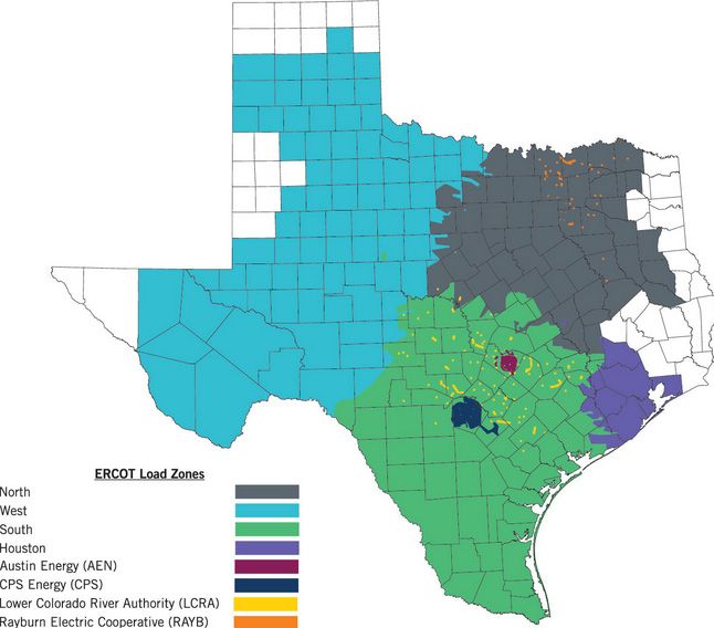
Appl. Sci. 2021, 11, 7039                                                                                            2 of 15

                            yielding 5-min locational marginal prices (LMPs) for each electrical bus within the market.
                            The SCED process seeks to minimize offer-based costs, subject to power balance and
                            network constraints. The zonal settlement price for a load-serving entity’s real-time energy
                            purchase is a load-weighted average of all 5-min LMPs in a load zone, which is converted
                            to 15-min values or hourly values by ERCOT.
                                  Economic merit order effects attributable to renewable energy generation have been
                            analyzed for many of the world’s competitive wholesale markets using linear regression
                            models. These include studies of the market in Spain [2], Germany [3–6], Denmark [7,8],
                            Italy [9], Australia [10], Ireland [11], the U.S. mid-continent or MISO [12,13], Texas [14–16],
                            PJM [17], the Pacific Northwest [18,19], and California [20]. Also, quantile regression ap-
                            proaches have been employed to study merit-order effects in Turkey [21] and Germany [22].
                                  Methodological Contribution. We explore this topic using hourly real-time price data for
                            the years 2015–2018 from the ERCOT market. Divided into eight zones—North, Houston,
                            South, West, Austin Energy, CPS Energy, Lower Colorado River Authority, and Ray-
                            burn Electric Cooperative—ERCOT serves the electrical needs of the largest electricity-
                            consuming state in the U.S.; it accounts for about 8% of the nation’s total electricity gen-
                            eration, and is repeatedly cited as North America’s most successful attempt to introduce
                            competition in both generation and retail segments of the power industry (Distributed En-
                            ergy Financial Group, 2015). In the interests of brevity, we report the findings for Houston,
                            Austin, and West regions, since the results from the other regions are similar.
                                  To the best of our knowledge, this study is the first attempt at developing a latent-
                            factor system-wide model for estimating the merit-order effects of baseload and renewable
                            energy generation. While we use the Texas energy market to exemplify the methodology,
                            the models developed here are readily applicable to other markets as well. Moreover, while
                            we focus on real-time prices, the methodology readily lends itself to the study of day-ahead
                            prices as well.
                                  Section 2 describes the data and variables used in the study. The system-wide latent
                            factor model for prices is detailed in Section 3. Section 4 provides the results, followed by a
                            discussion and conclusion in Section 5.

                            2. Data and Variables
                                This section describes the data used in the analytic models, including the geographical
                            scope and sample period.

                            2.1. Geographical Scope
                                 The current ERCOT market with its eight zones is the focus of the paper; see Figure 1
                            for a map of ERCOT. The North and Houston zones account for about 37% and 27%,
                            respectively, of ERCOT market energy sales, while the South and West zones contribute
                            12% and 9%. Further, these four zones account for nearly all of the state’s retail competition,
                            and most of the competitive generation resides within these zones.
A Latent-Factor System Model for Real-Time Electricity Prices in Texas
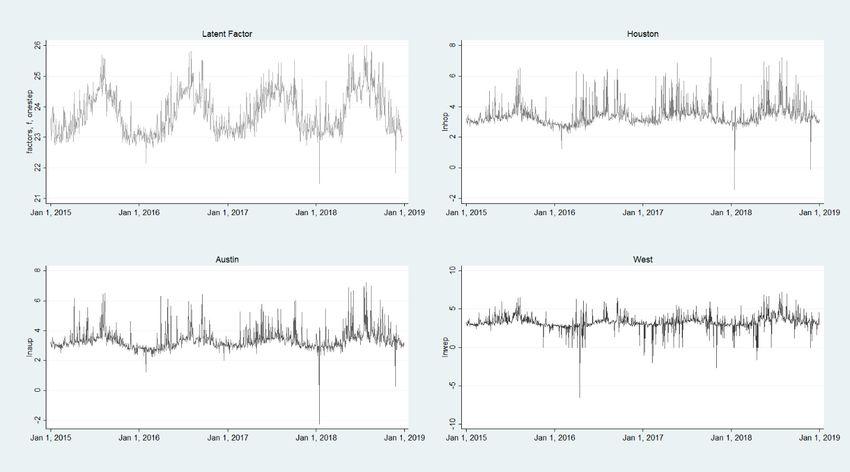
Appl. Sci. 2021, 11, 7039                                                                                                   3 of 15

Appl. Sci. 2021, 11, 7039     and the other two correspond to peak hours. There is nothing special about the specific
                                                                                                                3 of 15
                              hours we chose to work with; a similar analysis with other hours yields the same overall
                              conclusions reported here.

                              Figure 1. The eight ERCOT zones (Source: www.ercot.com, accessed on 18 July 2020).
                             Figure 1. The eight ERCOT zones (Source: www.ercot.com, accessed on 18 July 2020).

                                   TablePeriod
                             2.2. Sample  1 provides   the summary statistics for the prices ($/MWH) for the three hours
                                                 and Variables
                              andThe
                                   the sample
                                       three zones,  respectively.     The corresponding
                                                period starts on 1 January    2015 and ends time-series plots of2018.
                                                                                               on 31 December    the nine series,
                                                                                                                      Thus, we
                              shown
                             have     in red,
                                   a very     appear
                                          large       insince
                                                dataset  Figureall2.the
                                                                      Ineight
                                                                         the analysis, however,
                                                                              price series        we work
                                                                                           will appear     withasthe
                                                                                                       together      natural log
                                                                                                                   endogenous
                              of the price
                             variables     data.
                                       in the multivariate response matrix.
                                  As noted earlier, we discuss at length the results for the following three zones: Hous-
                              Table
                             ton,   1. Summary
                                  Austin,       statistics
                                          and the          of the hourly prices
                                                  West. Additionally,           ($/MWH)
                                                                          we examine theformerit-order
                                                                                            Houston, Austin,
                                                                                                       effectsand the West.
                                                                                                               stemming  from
                             three hours in a 24-h cycle:  4:00 a.m., 12:00 p.m.
                                                        Mean                 S.D. and, 4:00 p.m.Min
                                                                                                 The first is off-peak
                                                                                                                     Maxand the
                             other two correspond to peak hours. There is nothing special about the specific hours we
                                                                           Houston
                             chose to work with; a similar analysis with other hours yields the same overall conclusions
                                   4:00 a.m.            16.40                 5.83            −14.83                75.66
                             reported here.
                                  12:00 p.m.            31.13                47.95              9.59               1110.26
                                  Table 1 provides the summary statistics for the prices ($/MWH) for the three hours
                                   4:00three
                             and the     p.m.zones, respectively.
                                                        47.54                99.10
                                                                   The corresponding            0.24 plots of the1348.34
                                                                                         time-series                nine series,
                                                                            Austin
                             shown in red, appear in Figure 2. In the analysis, however, we work with the natural log of
                                   4:00data.
                             the price   a.m.           16.14                 6.31            −14.89                97.65
                                  12:00 p.m.            27.00                18.18              6.72                338.09
                             Table 4:00  p.m. statistics42.38
                                   1. Summary            of the hourly prices85.96              0.11 Austin, and the
                                                                              ($/MWH) for Houston,                 1348.11
                                                                                                                      West.
                                                                             West
                                                       Mean                  S.D.              Min                  Max
                                   4:00 a.m.            17.79                14.82            −15.56                132.71
                                  12:00 p.m.            27.55              Houston
                                                                             23.43            −16.88                408.91
                                  4:00 a.m.             16.40                5.83             −14.83                75.66
                                   4:00 p.m.            43.23                88.60            −15.67               1384.76
                                 12:00 p.m.             31.13                47.95                9.59              1110.26
                                  4:00 p.m.             47.54                99.10                0.24              1348.34
                                    One of the insights we hope to gain Austin
                                                                            is to see how the one-hour-ahead in-sample esti-
                              mates   ofa.m.
                                   4:00   the latent factor time series track6.31
                                                          16.14                                 −14.89
                                                                               the price plots in Figure 2. If we can    show that
                                                                                                                      97.65
                                  12:00
                              there  is ap.m.             27.00between the estimated
                                          strong correlation                 18.18                6.72 series and the338.09
                                                                                        latent factor                  price series,
                              then4:00
                                    thatp.m.
                                           bodes well for42.38
                                                           the estimation of85.96
                                                                              merit-order effects0.11
                                                                                                    from alternative1348.11
                                                                                                                       energy and
                                                                             West
                              baseload    generation. On17.79
                                   4:00 a.m.
                                                           the other hand, if14.82
                                                                              there is a very weak   relationship between
                                                                                                −15.56               132.71
                                                                                                                              latent
                              factors  and
                                  12:00 p.m. the price  series,
                                                          27.55 then exogenous
                                                                             23.43factors should   suffice
                                                                                                −16.88      in understanding
                                                                                                                     408.91      the
                              fluctuations
                                   4:00 p.m. in the price43.23
                                                           data.             88.60              −15.67              1384.76
A Latent-Factor System Model for Real-Time Electricity Prices in Texas
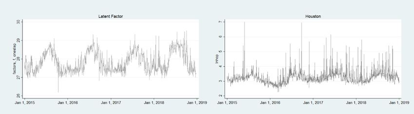
Appl. Sci. 2021, 11, 7039                                                                                                     4 of 15

                -20 0 20 40 60 80
                   Price ($/MWH)
                           1000
                Price ($/MWH)
                     5000
                   500 1000 1500
                Price ($/MWH)
                        0   50 100
                   Price ($/MWH)
                -50    0
                0 100 200 300 400
                 Price ($/MWH)
                   500 1000 1500
                Price ($/MWH)
                        0
                -50 0 50 100 150
                   Price ($/MWH)
                0 100 200 300 400
                 Price ($/MWH)
                   500 1000 1500
                Price ($/MWH)
                        0

      Figure 2. Time-series
      Figure 2. Time-series plots
                            plots of
                                  of the
                                     the actual
                                         actual prices
                                                prices (solid
                                                       (solid red
                                                              red line)
                                                                  line) and
                                                                        and model
                                                                            model predicted
                                                                                  predicted prices
                                                                                            prices (dash
                                                                                                   (dash grey
                                                                                                         grey line)
                                                                                                              line) in
                                                                                                                    in Houston,
                                                                                                                       Houston,
      Austin, and the West for the hours 4:00 a.m., 12:00 p.m. and 4:00 p.m.
      Austin, and the West for the hours 4:00 a.m., 12:00 p.m. and 4:00 p.m.

                                          A brief
                                          One   of discussion of we
                                                   the insights  eachhope
                                                                      of the
                                                                           toindependent   variables
                                                                              gain is to see how thenow   follows. Thesein-sample
                                                                                                      one-hour-ahead      variables
                                     were
                                     estimates of the latent factor time series track the price plots in Figure 2. If we cantables,
                                           selected  based  on  careful  data exploration  via summary    plots/correlation   show
                                     practical
                                     that thereconsiderations  of data size,
                                                is a strong correlation      modeling
                                                                         between       aims, and computational
                                                                                  the estimated                  complexities.
                                                                                                 latent factor series          Ad-
                                                                                                                      and the price
A Latent-Factor System Model for Real-Time Electricity Prices in Texas
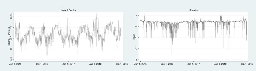
Appl. Sci. 2021, 11, 7039                                                                                               5 of 15

                            series, then that bodes well for the estimation of merit-order effects from alternative energy
                            and baseload generation. On the other hand, if there is a very weak relationship between
                            latent factors and the price series, then exogenous factors should suffice in understanding
                            the fluctuations in the price data.
                                  A brief discussion of each of the independent variables now follows. These vari-
                            ables were selected based on careful data exploration via summary plots/correlation tables,
                            practical considerations of data size, modeling aims, and computational complexities. Addi-
                            tionally, price formation in the ERCOT market has been analyzed in a variety of antecedent
                            studies using many of the same data sources and variables employed in this study [14–16].
                                  The exogenous variables used in this study are split into those that appear in the
                            observation and latent factor equations, respectively; these equations are detailed in the
                            next section.
                                  Observation Equation Exogenous Variables. Wind generation, nuclear generation, solar
                            generation, the Henry Hub gas price, and a dummy variable for spikes in prices that
                            exceed $500 MWH are the exogenous variables. ERCOT analysts have noted that industrial
                            customers tend to significantly scale back when prices exceed USD 500. So, a binary
                            dummy variable for extreme price spikes is used. The solar generation variable and the
                            dummy variable do not appear in the 4:00 a.m. equations. We downloaded daily natural
                            gas prices for Henry Hub from the DOE/EIA (See: http://www.eia.gov/dnav/ng/hist/
                            rngwhhdd.htm. Last accessed 18 July 2020). We use the Henry Hub price instead of the
                            local natural gas price (e.g., Houston Ship Channel) since the Henry Hub price is highly
                            correlated with the local natural gas price (r > 0.95). Finally, the latent factor variable, which
                            is estimated from within the system endogenously, appears as an exogenous variable in
                            the observation equation. All variables are on the natural log scale except, of course, the
                            dummy variable.
                                  Latent Factor Equation Exogenous Variables. Recall that the latent factors are unobserved
                            variables; there is no data for them. The parameters corresponding to these variables are
                            recursively estimated from within the system at each point in time, which leads to the
                            following intuition: if one could observe these latent causes, then they are most likely
                            going to be related to load and prices. For instance, power outages, erroneous short-
                            term weather forecasts, unanticipated transmission bottlenecks, etc., would most certainly
                            impact demand and price distributions across ERCOT. Therefore, we use system-wide
                            load (MWH) and lagged weighted price ($/MWH) across all eight zones as the exogenous
                            factors that could likely associate with the unobserved factor variables. Additionally, a
                            first-order autoregressive process for the latent factor is used. This allows us to capture
                            the potential lingering effects of hidden variables over time. As described in the next
                            section, while we could use higher-order lags, we do not do so in the interests of parsimony.
                            Also, the lagged weighted prices do capture some of the previous time period’s effect
                            on the latent factor. Note that the system-wide load is, in one sense, endogenous to the
                            observation equation via the latent factor. Finally, we work with the natural logs of all
                            these variables.

                            3. The Latent Factor Systems Model
                                 Following [23,24], suppose there are k endogenous variables. Let n f < k denote the
                            number of unknown or hidden latent factors. Then, the system of equations that represent
                            the prices in the k = 8 zones in ERCOT with n f = 1 is given by:

                                                      yt = λft + βxt + ut ft = δzt + ρft−1 + wt ,                          (1)

                            where the first equation is called the observation equation and the second is termed the
                            latent factor equation. The dimensions of the various quantities in Equation (1) are: yt is
                            a k × 1 vector of endogenous variables; λ is n f × n f ; ft is n f × n f ; β is a k × n x vector of
                            parameters; xt is an n x × 1 vector of exogenous variables; ut is a k × 1 vector of random
                            errors that are assumed to be normally distributed with mean zero and unknown standard
                            deviation σu ; δ is an n f × nz of parameters; zt is an nz × 1 vector of exogenous variables;
A Latent-Factor System Model for Real-Time Electricity Prices in Texas
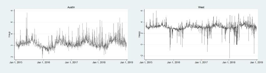
Appl. Sci. 2021, 11, 7039                                                                                              6 of 15

                            ρ is an n f × n f matrix of parameters; and wt is an n f × 1 vector of random errors that is
                            normally distributed with mean zero and unknown standard deviation σw .
                                  It is possible to introduce another Equation in (1) that represents an autoregressive
                            structure for the observation error ut . However, this leads to a larger number of parameters
                            than is dictated in most applications. Moreover, convergence issues abound when the
                            parameter space and the sample size are large. As it is, the class of models contained
                            in (1) is quite rich. By appropriately restricting n f , p and q, we can obtain Zellner’s
                            Seemingly Unrelated Regression model, Vector Autoregressive models; Dynamic Factors
                            with Errors models, etc; see, for example [25,26]. Williamson et al. [1] developed an
                            alternative Bayesian latent factor model, using nonparametric methods, that complements
                            the latent factor model in Equation (1).
                                  We could also add higher-order latent factors (n f > 1), but again we err on the side of
                            parsimony. Indeed, we could also increase the dimension of the autoregressive component
                            of the latent factor vector ft which we have set as an AR(1) process. But we refrain from
                            doing this since we also include the lagged weighted price of all the zones as an exogenous
                            variable in the vector zt ; i.e., we allow the weighted values of lagged prices from the eight
                            zones to guide the hidden factors that could drive each zone’s price in the observation
                            equation where these prices are endogenous in the system given in (1).
                                  Thus, yt is the endogenous matrix of prices from the eight zones; xt contains the
                            exogenous variables wind, nuclear and solar generation, where the last one appears only
                            in the sunlight hours; the Henry Hub gas price; and a dummy variable for real-time prices
                            exceeding USD 500, which will not appear in the night and early morning hours since prices
                            do not rise to very high levels at these times. The endogenous factor variable ft also appears as
                            an exogenous input in the observation equation. The implication is that these hidden factors
                            could influence prices throughout the day. In the latent factor equation, the exogenous
                            variables in zt use system-wide load (MWH) and lagged weighted price (USD/MWH)
                            across all eight zones; these are contemporaneous in time. Additionally, we assume the
                            latent factor follows a first-order autoregressive process. Since we separate our analysis for
                            each hour of the day, the lagged variables are the variables of the previous day. Since ft
                            enters the observation equation exogenously, the system-wide load affects system-wide
                            prices via ft . Lastly, the AR(1) specification for ft in the second equation captures the lagged
                            nature of hidden factors; for example, poor weather forecasts, which could be one of the
                            latent factors, tend to be contiguous over time.
                                  The maximum likelihood estimates (MLEs) for all the parameters (including δ and ρ)
                            are found via an iterative method that combines the two algorithms developed in [27,28].
                            All analyses were conducted in STATA.

                            4. Results
                                 Here, we report and discuss the results for three regions: Houston, Austin, and West;
                            details on all other regions are available on request. Where appropriate, we highlight the
                            empirics from the other regions as well. For the three regions, we report the results for
                            4:00 a.m., 12:00 p.m., and 4:00 p.m.; these are representative of the other off-peak and peak
                            hours. Thus, we estimate Equation (1) nine times since we have nine models in total. We
                            have the following major results.
                                 Wald Test. This test has a chi-square distribution. It tests the null hypothesis of whether
                            or not all the unknown parameters in the observation and latent factor equations are jointly
                            significant; this is similar to the F-test in multiple linear regression. For all nine models, the
                            Wald Statistic soundly rejects the null hypothesis at any significance level (p < 0.00001).
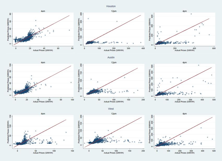
                                 Actual versus predicted price series. Consider Figure 3 which shows the actual and pre-
                            dicted series. As expected, there are some outliers in the data, especially during the 4:00 p.m.
                            hour for all three zones. Also, again consider Figure 2. Note that the predicted time series,
                            shown in grey, track the original price series in red quite well for the three different hours,
                            barring the time points corresponding to the outliers.
A Latent-Factor System Model for Real-Time Electricity Prices in Texas
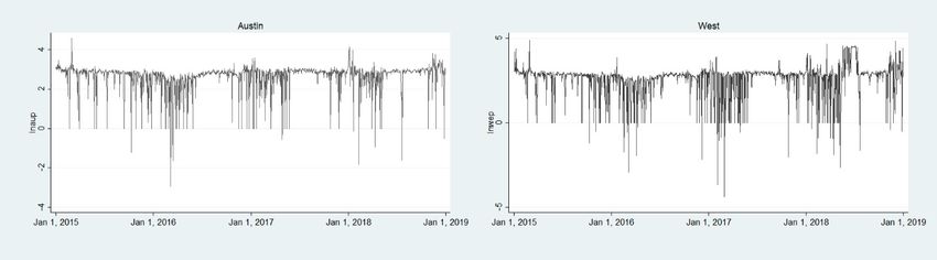
Appl. Sci. 2021, 11, 7039                                                                                                                              7 of 15

      Figure 3. Scatter plots of actual and predicted prices, along with 45-degree lines, in Houston, Austin, and the West for the
      Figure 3. Scatter plots of actual and predicted prices, along with 45-degree lines, in Houston, Austin, and the West for the
      hours 4:00 a.m., 12:00 p.m., and 4:00 p.m.
      hours 4:00 a.m., 12:00 p.m., and 4:00 p.m.

                                        Correlations
                                        Correlationsbetween
                                                         betweenactual
                                                                    actualprice
                                                                            priceseries
                                                                                   seriesand estimated
                                                                                           and  estimated factor    series
                                                                                                               factor   series. Table    2 shows
                                                                                                                                ft . Table  2 showsthethe
                                                                                                                                                       corre-
                                                                                                                                                           cor-
                                  lations  between     each   of  the  price  series   from   all  eight   zones     for  the
                                  relations between each of the price series from all eight zones for the three hours. They arethree    hours.  They   are   all
                                  positively   correlated     to  the  predicted    latent   factors.    We    highlighted
                                  all positively correlated to the predicted latent factors. We highlighted the correlations for the   correlations   for   the
                                  regions   Houston,
                                  the regions    Houston, Austin,    and West
                                                                Austin,           in Table
                                                                           and West           2 in 2order
                                                                                         in Table             to emphasize
                                                                                                       in order      to emphasize  two points.    First,First,
                                                                                                                                         two points.      note
                                  that the  West   zone     has  the  weakest    correlation    during      the   peak
                                  note that the West zone has the weakest correlation during the peak hours of 12:00 p.m.hours     of  12:00  p.m.  and   4:00
                                  p.m., compared
                                  and 4:00             to other regions.
                                              p.m., compared                 Thisregions.
                                                                      to other     is because    of the
                                                                                               This       larger impact
                                                                                                      is because       of theoflarger
                                                                                                                                   wind generation
                                                                                                                                           impact of in windthe
                                  West  duringinthese
                                  generation         the hours,     compared
                                                           West during       theseto hours,
                                                                                      other zones.
                                                                                               compared Second,  to consider
                                                                                                                     other zones.Figures    4–6. Each
                                                                                                                                         Second,        com-
                                                                                                                                                    consider
                                  prises
                                  Figures four
                                            4–6.plots.
                                                   EachFor   the sake of
                                                           comprises        clarity,
                                                                          four  plots.letFor
                                                                                           us the
                                                                                              focus    on of
                                                                                                    sake   justclarity,
                                                                                                                  Figurelet 6 corresponding
                                                                                                                              us focus on justtoFigure
                                                                                                                                                     the 4:00  6
                                  p.m.  hour.  The    top  left plot  is the latent  factor   one-step-ahead          estimated
                                  corresponding to the 4:00 p.m. hour. The top left plot is the latent factor one-step-ahead         time  series. The  other
                                  three plots time
                                  estimated     in each   of theThe
                                                       series.     panels
                                                                       otherare the actual
                                                                              three   plots inprice
                                                                                                 each series
                                                                                                         of the forpanels
                                                                                                                     Houston,are Austin,
                                                                                                                                   the actualandprice
                                                                                                                                                   West.  The
                                                                                                                                                       series
                                  corresponding
                                  for Houston, Austin,correlations     between
                                                                and West.     Thethe    latent factor series
                                                                                    corresponding                  and these
                                                                                                          correlations            three price
                                                                                                                             between             seriesfactor
                                                                                                                                           the latent    from
                                  Table
                                  series 2and
                                           are:these
                                                 0.587,three
                                                          0.591,  andseries
                                                                price   0.457,from
                                                                                respectively.     It is 0.587,
                                                                                       Table 2 are:     evident      that and
                                                                                                                  0.591,   the latent
                                                                                                                                 0.457,factor    series struc-
                                                                                                                                          respectively.    It is
                                  turally
                                  evidentevolves
                                            that thelikelatent
                                                          the three
                                                                 factorprice   series,
                                                                          series         which are
                                                                                  structurally          representative
                                                                                                  evolves    like the three   of price
                                                                                                                                  the price    series
                                                                                                                                          series,     for are
                                                                                                                                                  which     the
                                  entire ERCOT system.
                                  representative                The presence
                                                      of the price     series forofthe
                                                                                    outliers   inERCOT
                                                                                          entire   the pricesystem.
                                                                                                                 series isThe
                                                                                                                            unavoidable
                                                                                                                                  presencein   ofthe ERCOT
                                                                                                                                                  outliers   in
                                  data. Thisseries
                                  the price    wouldisexplain       why some
                                                           unavoidable       in theof ERCOT
                                                                                      the correlations
                                                                                                 data. This   arewould
                                                                                                                    not as high
                                                                                                                             explain  as one
                                                                                                                                         whymight
                                                                                                                                                someexpect.
                                                                                                                                                       of the
                                  correlations
                                  We              are not
                                       experimented          as high
                                                          with          as one might
                                                                  higher-order     lags in expect.    We experimented
                                                                                             the autoregressive           error with     higher-order
                                                                                                                                  structure               lags
                                                                                                                                               for the latent
                                  in the series
                                  factor  autoregressive
                                                  in Equation  error
                                                                   (1).structure
                                                                         But suchfor anthe   latentin
                                                                                          increase    factor
                                                                                                         model   series  in Equation does
                                                                                                                     dimensionality        (1). But
                                                                                                                                                 notsuch
                                                                                                                                                      change an
                                  increase
                                  the overallin conclusions
                                                 model dimensionality          does not
                                                                 by much. Hence,        wechange
                                                                                            err on the theside
                                                                                                             overall    conclusions by much. Hence,
                                                                                                                   of parsimony.
                                  we err on the side of parsimony.
Appl.
Appl. Sci.
      Sci. 2021,
           2021, 11,
                 11, 7039
                     7039                                                                                                         88 of
                                                                                                                                     of 15
                                                                                                                                        15
Appl. Sci. 2021, 11, 7039                                                                                                          8 of 15

                                  Table 2. Correlations between the actual price series and estimated factor series for all zones.
                                  Table 2. Correlations between the actual price series and estimated factor series for all zones.
                                  Table 2. Correlations between the actual price series and estimated factor series for all zones.
                                               Austin Houston LCRA North                      RAYB      CPS       South         West
                                               Austin  Austin    Houston
                                                           Houston     LCRA LCRANorth  North RAYB RAYB CPS CPS SouthSouth        West
                                                                                                                                West
                                   4:00 a.m. 0.343           0.323      0.343      0.339      0.318     0.344     0.338         0.346
                                   4:004:00
                                  12:00 a.m.a.m. 0.343 0.3430.3230.323 0.343
                                         p.m.    0.532       0.473      0.5310.343 0.541
                                                                                   0.3390.339 0.318
                                                                                                  0.318 0.344
                                                                                              0.517        0.344
                                                                                                        0.504        0.338
                                                                                                                   0.338
                                                                                                                  0.428          0.346
                                                                                                                                0.346
                                                                                                                                0.365
                                      12:00 p.m.        0.532     0.473      0.531      0.541     0.517    0.504     0.428       0.365
                                  12:00          0.532
                                         p.m. 0.591          0.473      0.531      0.541       0.517    0.504      0.428        0.365
                                   4:004:00
                                        p.m.p.m.        0.5910.5870.587 0.5940.594 0.6180.618 0.593
                                                                                                  0.593 0.559
                                                                                                           0.559 0.533
                                                                                                                     0.533      0.457
                                                                                                                                 0.457
                                   4:00 p.m.     0.591       0.587      0.594      0.618       0.593    0.559      0.533
                                  Note: Certain values are bold in order to better understand the Figure 6 discussion.          0.457
                                  Note: Certain values are bold in order to better understand the Figure 6 discussion.
                                  Note: Certain values are bold in order to better understand the Figure 6 discussion.

          Figure 4. 4:00 a.m.—Latent Factor and Houston series (top left and right); Austin and West (Bottom left and right).
          Figure 4. 4:00 a.m.—Latent Factor and Houston series (top left and right); Austin and West (Bottom left and right).
          Figure 4. 4:00 a.m.—Latent Factor and Houston series (top left and right); Austin and West (Bottom left and right).

      Figure 5. 12:00 p.m.—Latent Factor and Houston price series (top left and right); Austin and West (Bottom left and right).
      Figure 5.
      Figure    12:00 p.m.—Latent
             5. 12:00 p.m.—Latent Factor
                                  Factor and
                                         and Houston
                                             Houston price
                                                     price series
                                                           series (top
                                                                   (top left
                                                                        left and
                                                                             and right);
                                                                                 right); Austin
                                                                                         Austin and
                                                                                                and West
                                                                                                    West (Bottom
                                                                                                         (Bottom left
                                                                                                                 left and
                                                                                                                      and right).
                                                                                                                          right).
Appl. Sci. 2021, 11, 7039                                                                                                                     9 of 15

      Figure 6. 4:00 p.m.—Latent Factor and Houston price series (top left and right); Austin and West (Bottom left and right).
      Figure 6. 4:00 p.m.—Latent Factor and Houston price series (top left and right); Austin and West (Bottom left and right).

                                       Significance
                                        Significance of    the latent
                                                        of the  latent factor
                                                                        factorcoefficient.
                                                                               coefficient.From
                                                                                              From Table
                                                                                                     Table3,3, the
                                                                                                                the endogenous
                                                                                                                     endogenous latent
                                                                                                                                   latent factor
                                                                                                                                          factor
                                 variable,
                                 variable, ft,, when
                                                   whenititappears
                                                               appearsasasanan  exogenous
                                                                                  exogenous    variable  in the
                                                                                                  variable        observation
                                                                                                             in the             equation
                                                                                                                      observation         is sta-
                                                                                                                                     equation   is
                                 tistically  significant     for  all the   nine models     (p <  0.00001).  This  result  confirms
                                  statistically significant for all the nine models (p < 0.00001). This result confirms one of        one of  the
                                 principal
                                  the principalassertions    in this
                                                     assertions    in paper,    namely
                                                                       this paper,   namelythat that
                                                                                                 therethere
                                                                                                        are hidden,    unobserved
                                                                                                              are hidden,           factors
                                                                                                                             unobserved      that
                                                                                                                                         factors
                                 influence     the distribution     of  real-time  prices    throughout    a  24-h  cycle across
                                  that influence the distribution of real-time prices throughout a 24-h cycle across all zones.   all zones. Da-
                                 mien
                                  Damienet al.   [29][29]
                                            et al.     dodonotnot
                                                                useuselatent  factors
                                                                         latent factorsinintheir
                                                                                             theirsystem-wide
                                                                                                    system-widepricepriceand
                                                                                                                          anddemand
                                                                                                                               demand ERCOT
                                                                                                                                         ERCOT
                                 model.
                                  model. ItIt is
                                               isevident
                                                  evidentfrom
                                                            from this
                                                                   this research
                                                                          research that
                                                                                   that latent
                                                                                         latent factors
                                                                                                  factors play
                                                                                                          play aa significant
                                                                                                                   significant role
                                                                                                                               role in
                                                                                                                                    in ERCOT’s
                                                                                                                                       ERCOT’s
                                 pricing
                                 pricing structure.
                                           structure.
                                 Table 3.
                                 Table    Coefficients for
                                       3. Coefficients for the
                                                           the Latent
                                                               Latent Factor
                                                                      Factor ft ..

                                              AustinAustin
                                                        HoustonHouston
                                                                    LCRA LCRANorth  NorthRAYB RAYB               CPSCPS        South
                                                                                                                              South         West
                                                                                                                                           West
                                  4:004:00
                                       a.m.a.m. 0.571 0.571
                                                          0.532 0.5320.5810.581 0.5330.533 0.510
                                                                                              0.510                 0.550
                                                                                                                 0.550          0.541
                                                                                                                              0.541         0.621
                                                                                                                                           0.621
                                     12:00 p.m.
                                 12:00 p.m. 0.266     0.266
                                                          0.284 0.2840.2730.273 0.2230.223    0.204
                                                                                           0.204                    0.272
                                                                                                                 0.272          0.268
                                                                                                                              0.268         0.292
                                                                                                                                           0.292
                                      4:00 p.m.       0.433     0.430     0.441      0.427    0.425                 0.423       0.412       0.461
                                  4:00 p.m. 0.433         0.430      0.441      0.427      0.425                 0.423        0.412        0.461
                                 Note: All coefficients have p-values < 0.00001. The latent factor is a vector quantity; hence it appears in bold font
                                 Note:   All coefficients
                                  to be consistent with thehave  p-values
                                                            notation       < 0.00001.
                                                                     in Section 3.    The latent factor is a vector quantity; hence it appears
                                 in bold font to be consistent with the notation in Section 3.
                                       The marginal effects of the exogenous variables. Consider Tables 4–6 which show the max-
                                  imum   likelihood
                                       The  marginal estimates    (MLEs)
                                                     effects of the       for coefficients
                                                                    exogenous              that appear
                                                                               variables. Consider      in the
                                                                                                    Tables  4–6observation
                                                                                                                which showand
                                                                                                                            the latent
                                                                                                                                 max-
                                         equations   in (1); the   corresponding    p-values;
                                 imum likelihood estimates (MLEs) for coefficients that appear in the observation and for
                                  factor                                                      and  the 95%   confidence intervals  la-
                                  Hours
                                 tent     4:00equations
                                      factor   a.m., 12:00inp.m.,   andcorresponding
                                                             (1); the   4:00 p.m., respectively,
                                                                                        p-values; for
                                                                                                  andthe
                                                                                                       thethree
                                                                                                            95% zones.
                                                                                                                confidence intervals
                                 for Hours 4:00 a.m., 12:00 p.m., and 4:00 p.m., respectively, for the three zones.

                                 Table 4. ML coefficients for the 4:00 a.m. hour.

                                                       Coefficient              p-Value                    95% Confidence Intervals
                                                                            Latent Factor Equation
                                                           0.1681                 0.0030                   0.0579                    0.2783
                                  SystemLoad              1.6092                 0.00001                   1.3573                    1.8610
                                   Lag(WtPr)              −0.1248                 0.1660                   −0.3015                   0.0518
                                                                              Houston Equation
                                                           0.5331                0.00001                    0.5117                   0.5545
Appl. Sci. 2021, 11, 7039                                                                                          10 of 15

                            Table 4. ML coefficients for the 4:00 a.m. hour.

                                                     Coefficient           p-Value          95% Confidence Intervals
                                                                   Latent Factor Equation
                                   ft −1              0.1681                0.0030          0.0579            0.2783
                               SystemLoad             1.6092               0.00001          1.3573            1.8610
                                Lag(WtPr)             −0.1248              0.1660           −0.3015           0.0518
                                                                     Houston Equation
                                    ft                0.5331               0.00001          0.5117           0.5545
                                  Wind                −0.3570              0.00001          −0.4027          −0.3112
                                 Nuclear              −0.7034              0.00001          −0.9073          −0.4995
                                Henry Hub             1.1530               0.00001          0.9328           1.3733
                                                                      Austin Equation
                                    ft                0.5709               0.00001          0.5502           0.5917
                                  Wind                −0.3674              0.00001          −0.4143          −0.3204
                                 Nuclear              −0.7780              0.00001          −0.9948          −0.5612
                                Henry Hub             1.1212               0.00001          0.8919           1.3505
                                                                       West Equation
                                    ft                0.6207               0.00001          0.5831           0.6583
                                  Wind                −0.5517              0.00001          −0.6190          −0.4845
                                 Nuclear              −0.7153              0.00001          −0.9645          −0.4662
                                Henry Hub             1.1317               0.00001          0.8288           1.4345

                            Table 5. ML coefficients for the 12:00 p.m. sample.

                                                     Coefficient           p-Value          95% Confidence Intervals
                                                                   Latent Factor Equation
                                   ft −1              0.2240               0.00001          0.1412           0.3067
                               SystemLoad             2.0997               0.00001          1.8646           2.3348
                                Lag(WtPr)             −0.2542              0.0430           −0.4999          −0.0085
                                                                     Houston Equation
                                    ft                0.2845               0.00001          0.2713           0.2977
                                  Wind                −0.0943              0.00001          −0.1151          −0.0736
                                 Nuclear              −0.5532              0.00001          −0.6576          −0.4487
                                  Solar               0.0243                0.0630          −0.0013          0.0500
                                Henry Hub             0.6154               0.00001          0.4786           0.7522
                                 Dummy                2.4006               0.00001          2.1030           2.6982
                                                                      Austin Equation
                                    ft                0.2661               0.00001          0.2559           0.2763
                                  Wind                −0.1432              0.00001          −0.1603          −0.1261
                                 Nuclear              −0.4445              0.00001          −0.5392          −0.3497
                                  Solar               0.0090                0.4140          −0.0126          0.0307
                                Henry Hub             0.6454               0.00001          0.5272           0.7636
                                 Dummy                1.2841               0.00001          1.0444           1.5237
                                                                       West Equation
                                    ft                0.2916               0.00001          0.2684           0.3148
                                  Wind                −0.2826              0.00001          −0.3155          −0.2497
                                 Nuclear              −0.3945              0.00001          −0.5201          −0.2689
                                  Solar               0.0093                0.6340          −0.0292          0.0478
                                Henry Hub             0.5949               0.00001          0.4013           0.7885
                                 Dummy                0.9767               0.00001          0.4842           1.4692
Appl. Sci. 2021, 11, 7039                                                                                             11 of 15

                            Table 6. ML coefficients for the 4:00 p.m. sample.

                                                    Coefficient           p-Value            95% Confidence Intervals
                                                                  Latent Factor Equation
                                   ft −1               0.1326              0.0010            0.0571             0.2080
                               SystemLoad              1.8513             0.00001            1.6365             2.0661
                                Lag(WtPr)              0.2243              0.0010            0.0899             0.3587
                                                                    Houston Equation
                                    ft                0.4302              0.00001           0.4117             0.4487
                                  Wind                −0.1761             0.00001           −0.2085            −0.1438
                                 Nuclear              −0.7292             0.00001           −0.8540            −0.6043
                                  Solar               0.0703              0.00001           0.0413             0.0993
                                Henry Hub             0.3608              0.00001           0.2006             0.5211
                                 Dummy                2.0212              0.00001           1.8419             2.2004
                                                                     Austin Equation
                                    ft                0.4334              0.00001           0.4169             0.4499
                                  Wind                −0.2222             0.00001           −0.2520            −0.1924
                                 Nuclear              −0.6829             0.00001           −0.8060            −0.5599
                                  Solar               0.0482              0.00001           0.0211             0.0752
                                Henry Hub             0.3430              0.00001           0.1933             0.4927
                                 Dummy                1.8556              0.00001           1.6916             2.0195
                                                                      West Equation
                                    ft                0.4615              0.00001           0.4307             0.4922
                                  Wind                −0.4326             0.00001           −0.4827            −0.3825
                                 Nuclear              −0.5835             0.00001           −0.7351            −0.4319
                                  Solar               0.0473               0.0320           0.0040             0.0906
                                Henry Hub             0.5272              0.00001           0.2893             0.7651
                                 Dummy                1.2448              0.00001           0.9629             1.5268

                                  Since we are dealing with the natural logs of all the variables, the MLEs represent
                            elasticities. We first describe some overarching conclusions from all three tables here,
                            saving for later the discussion of the merit-order effects.
                                  First, from the latent factor equations for all three hours and zones, system-wide
                            load (SystemLoad) positively and significantly impacts the hidden factors. Second, lagged
                            weighted price (LagWtPr) is not significant in the off-peak hour but is significant during
                            the peak hours. Interestingly, it impacts the hidden factors negatively at the noon hour
                            and positively at the 4:00 p.m. hour. Third, the lagged latent factor variable is positive and
                            statistically significant at all three hours for all three zones in the latent factor equation. In
                            conjunction with the plots shown in Figures 4–6, this further confirms the importance of
                            the latent factor dynamics on energy prices in all eight zones. Fourth, from the observation
                            equation for the three zones, during all three hours, as expected, wind generation and
                            nuclear generation have negative elasticities, and Henry Hub gas has positive elasticity.
                            Fifth, solar generation is a mixed bag, largely because this resource is still growing in Texas,
                            and as such its data are non-stationary. Thus, solar generation is not significant at 12:00 p.m.
                            and its elasticities are positive and weak at 4:00 p.m. Finally, the impact of extreme spikes
                            in real-time prices (the dummy variable) at 12:00 p.m. and 4:00 p.m. is highly significant in
                            all three zones.
                                  System-wide merit-order effects. To best understand the merit-order effects shown as
                            elasticities in Tables 4–6, consider the price boxplots shown in Figure 7. The top, middle
                            and bottom panels, corresponding to hours 4:00 a.m. 12:00 p.m., and 4:00 p.m., respectively,
                            have three boxplots in each panel. On the X-axis, the box titled “Before Price” is the
                            group of mean prices in the eight ERCOT zones before accounting for any merit-order
                            effect. The second and third boxes are the change in mean prices after accounting for
                            merit-order effects in wind and nuclear generation, respectively. The Y-axis represents
                            the mean price values ($/MWH). Each value on this axis is the mean price from each of
                            the eight zones during the years 2015–2018. Focus on the 4:00 a.m. panel at the top. The
                            interquartile range (IQR) of the mean prices of the eight zones in ERCOT at this hour is
                            $16.18 to $16.61; see the left-most box in blue. Next, assume wind generation increases
Appl. Sci. 2021, 11, 7039                                                                                                 12 of 15

                             by 10%. Using the MLE estimates of the price elasticities for wind generation for each of
Appl. Sci. 2021, 11, 7039    the eight zones from our latent-factor system model, we adjust the mean prices in the       12 blue
                                                                                                                            of 15
                             box and construct the resulting change in prices due to increased wind generation. The
                             corresponding distribution of the adjusted mean prices in ERCOT is shown as the second
                             box
                             in    in From
                                red.  red. From  the caption,
                                            the caption,       the for
                                                          the IQR  IQRtheforprices,
                                                                             the prices,
                                                                                    after after accounting
                                                                                           accounting       for increased
                                                                                                      for increased  windwind
                                                                                                                           gen-
                             generation, is between $15.59 and $16.07. Finally, we do a similar adjustment to energy
                             eration, is between $15.59 and $16.07. Finally, we do a similar adjustment to energy prices
                             prices using the parameter estimates for nuclear generation; this is shown as the green box
                             using the parameter estimates for nuclear generation; this is shown as the green box in the
                             in the top row of Figure 7. The IQR is between $14.98 and $15.42. Observing the three
                             top row of Figure 7. The IQR is between $14.98 and $15.42. Observing the three panels, it
                             panels, it is also interesting to note that there is less volatility in the mean prices in the
                             is also interesting to note that there is less volatility in the mean prices in the entire ERCOT
                             entire ERCOT system during the off-peak hour.
                             system during the off-peak hour.

                            Figure 7. ERCOT merit-order effects for wind and nuclear generation.
                            Figure 7. ERCOT merit-order effects for wind and nuclear generation.

                                   Consider
                                   Consider the
                                              the middle
                                                  middlepanel
                                                           panelwhich
                                                                  whichcorresponds
                                                                        correspondstotothe
                                                                                         the12:00 p.m.
                                                                                              12:00 p.m. hour. While
                                                                                                            hour.    the the
                                                                                                                  While   re-
                             duction  in energy  prices is less now, wind and nuclear  generation   still have a measurable
                             reduction in energy prices is less now, wind and nuclear generation still have a measurable
                             impact on real-time prices in ERCOT as a whole. Also, there is more volatility in real-time
                             prices during this peak hour.
                                   Finally, the bottom panel shows the impact on prices due to the merit-order effects
                             at 4:00 p.m. Nuclear generation is much more influential than wind at this hour of the day;
                             its boxplot barely intersects with the boxplot from wind generation. Also, the volatility in
                             ERCOT’s prices is lesser at 4:00 p.m. when compared to 12:00 p.m.
Appl. Sci. 2021, 11, 7039                                                                                           13 of 15

                            impact on real-time prices in ERCOT as a whole. Also, there is more volatility in real-time
                            prices during this peak hour.
                                  Finally, the bottom panel shows the impact on prices due to the merit-order effects at
                            4:00 p.m. Nuclear generation is much more influential than wind at this hour of the day;
                            its boxplot barely intersects with the boxplot from wind generation. Also, the volatility in
                            ERCOT’s prices is lesser at 4:00 p.m. when compared to 12:00 p.m.

                            5. Conclusions
                                  This paper demonstrated the relevance of latent factors on real-time energy prices
                            using a system-wide approach. The ERCOT system served as the case study. Using
                            energy prices from eight inter-connected zones as endogenous variables, we found that
                            hidden factors significantly impact the merit-order effects of baseload and renewable
                            energy generation.
                                  The latent-factor approach developed here can be improved and extended.
                            Damien et al. [29] use a hierarchical Bayesian approach to compare the impact of day-
                            ahead and real-time prices on wholesale demand in ERCOT. However, they do not model
                            latent factors. This paper clearly shows the importance of accounting for such factors. A
                            Bayesian latent factor system-wide model for prices and/or demand is possible in principle;
                            see [30]. However, the challenges are formidable. First, since the parameter space is very
                            large, convergence issues will be a difficult problem to overcome. Concurrently, while
                            studying energy prices or demand, the attendant datasets tend to be very large, as in this
                            paper. This too will add to convergence issues since the likelihood function will have to be
                            evaluated many-fold in any Markov chain Monte Carlo scheme that is required to obtain
                            posterior distributions.
                                  Another future topic for research that this paper proposes is to model the system of
                            equations in Equation (1) via non-normal errors. For example, Williamson et al. [1] use a
                            nonparametric error distribution—the Indian Buffet Process—to develop a new class of
                            latent factor models. But with large datasets, such nonparametric approaches are even
                            more computationally involved compared to parametric formulations.
                                  Why should a non-normal error structure matter in the context of energy prices,
                            and in the estimation of merit-order effects? Recent studies [21,22] have shown that
                            prices have asymmetric distributions with large kurtosis. Subsequently, error distributions
                            from normal linear models tend to be non-normal heteroscedastic and autocorrelated.
                            Hence, quantile regressions have been proposed and exemplified in the energy literature.
                            However, there is a trade-off. Because of the mathematics underlying them, quantile
                            regressions are essentially single-equation models. Thus, the prices of each of ERCOT’s
                            eight zones can be modeled separately using quantile regressions; see [31]. But the results
                            in this paper clearly demonstrate the importance of treating the eight zones as part of
                            an interconnected system so that we can better understand how latent factors influence
                            prices jointly. This leads to an open question: how should one construct a system-wide,
                            latent-factor quantile regression model that is equivalent to Equation (1) in this paper? This
                            is a very challenging problem for multiple reasons. For example, consider a bivariate time-
                            series that represent prices from, say two of ERCOT’s eight zones. Further, suppose the error
                            term in the observation model in Equation (1) follows a bivariate skew-t distribution since
                            this distribution allows for varying degrees of skewness. How should one jointly model
                            the quantiles of this bivariate distribution as functions of latent factors and exogenous
                            variables? The answer is not at all evident even in this simple bivariate setup. Therefore,
                            instead of multivariate quantile regression systems, we believe, as a first step, it may be
                            easier to recast Equation (1) using nonparametric prior distributions. Indeed, this could
                            also lead to stronger correlations between the factor and price series since nonparametric
                            priors can better treat outliers. The resulting estimation of the merit-order effects in energy
                            markets would be a useful advancement.
Appl. Sci. 2021, 11, 7039                                                                                                              14 of 15

                                  Author Contributions: Conceptualization, P.D. and J.Z.; methodology, P.D.; software, K.H.C.; valida-
                                  tion, K.H.C., P.D. and J.Z.; formal analysis, K.H.C. and P.D.; investigation, P.D. and J.Z.; resources, J.Z.;
                                  data curation, K.H.C. and J.Z.; writing—original draft preparation, K.H.C., P.D. and J.Z.; writing—
                                  review and editing, K.H.C., P.D. and J.Z.; visualization, K.H.C.; supervision, P.D. and J.Z.; project
                                  administration, K.H.C. and P.D. All authors have read and agreed to the published version of
                                  the manuscript.
                                  Funding: This research received no external funding.
                                  Institutional Review Board Statement: Not Applicable.
                                  Informed Consent Statement: Not Applicable.
                                  Data Availability Statement: Data presented in this study are available from the third author
                                  upon request.
                                  Conflicts of Interest: The authors declare no conflict of interest.

References
1.    Williamson, S.; Zhang, M.; Damien, P. A new class of time-dependent latent factor models with applications. J. Mach. Learn. Res.
      2020, 21, 1–24.
2.    Gelabert, L.; Labandeira, X.; Linares, P. An ex-post analysis of the effect of renewable and cogeneration on Spanish electricity
      prices. Energy Econ. 2011, 22, 559–565. [CrossRef]
3.    Sensfuß, F.; Ragwitz, M.; Genoese, M. The merit-order effect: A detailed analysis of the price effect of renewable electricity
      generation on spot market prices in Germany. Energy Policy 2008, 36, 3086–3094. [CrossRef]
4.    Ketterer, J.C. The impact of wind power generation on the electricity price in Germany. Energy Econ. 2014, 44, 270–280. [CrossRef]
5.    Cludius, J.; Hermann, H.; Matthes, F.C.; Graichen, V. The merit order effect of wind and photovoltaic electricity generation in
      Germany 2008–2016: Estimation and distributional implications. Energy Econ. 2014, 44, 302–313. [CrossRef]
6.    Paraschiv, F.; Erni, D.; Pietsch, R. The impact of renewable energies on EEX day-ahead electricity prices. Energy Policy 2014, 73,
      196–210. [CrossRef]
7.    Munksgaard, J.; Morthorst, P.E. Wind power in the Danish liberalized power market–Policy measures, price impact, and investor
      incentives. Energy Policy 2008, 36, 3940–3947. [CrossRef]
8.    Jacobsen, H.K.; Zvingilaite, E. Reducing the market impact of large shares of intermittent energy in Denmark. Energy Policy 2010,
      38, 3403–3413. [CrossRef]
9.    Clo, S.; Cataldi, A.; Zoppoli, P. The merit-order effect in the Italian power market: The impact of sola and wind generation on
      national wholesale electricity prices. Energy Policy 2015, 77, 79–88. [CrossRef]
10.   Cutler, N.J.; MacGill, I.F.; Outhred, H.R.; Boerema, N.D. High penetration wind generation impacts on spot prices in the Australian
      national electricity market. Energy Policy 2011, 39, 5939–5949. [CrossRef]
11.   Denny, E.; O’Mahoney, A.; Lannoye, E. Modelling the impact of wind generation on electricity market prices in Ireland: An
      econometric versus unit commitment approach. Renew. Energy 2017, 104, 109–119. [CrossRef]
12.   Quint, D.; Dahlke, S. The impact of wind generation on wholesale electricity market prices in the midcontinent independent
      system operator energy market: An empirical investigation. Energy 2007, 169, 456–466. [CrossRef]
13.   Zarnikau, J.; Tsai, C.H.; Woo, C.K. Determinants of the wholesale prices of energy and ancillary services in the US Midcontinent
      electricity market. Energy 2020. [CrossRef]
14.   Zarnikau, J.; Woo, C.K.; Zhu, S.S. Zonal merit-order effects of wind generation development on day-ahead and real-time electricity
      market prices in Texas. J. Energy Mark. 2016, 9, 17–47. [CrossRef]
15.   Zarnikau, J.; Woo, C.K.; Zhu, S.S.; Baldick, R.; Tsai, C.H.; Meng, J. Electricity market prices for day-ahead ancillary services and
      energy: Texas. J. Energy Mark. 2018, 12, 1–32. [CrossRef]
16.   Zarnikau, J.; Woo, C.K.; Zhu, S.S.; Tsai, C.H. Market price behavior of wholesale electricity products: Texas. Energy Policy 2019,
      125, 418–428. [CrossRef]
17.   Gil, H.A.; Lin, J. Wind power and electricity prices at the PJM market. IEEE Trans. Power Syst. 2013, 28, 3945–3953. [CrossRef]
18.   Woo, C.K.; Zarnikau, J.; Kadish, J.; Horowitz, I.; Wang, J.; Olson, A. The impact of wind generation on wholesale electricity prices
      in the hydro-rich Pacific Northwest. IEEE Trans. Power Syst. 2013, 28, 4245–4253. [CrossRef]
19.   Woo, C.K.; Moore, J.; Schneiderman, B.; Olson, A.; Jones, R.; Ho, T.; Toyama, N.; Wang, J.; Zarnikau, J. Merit-order effects of
      day-ahead wind generation forecast in the hydro-rich Pacific Northwest. Electr. J. 2015, 28, 52–62. [CrossRef]
20.   Woo, C.K.; Moore, J.; Schneiderman, B.; Olson, A.; Jones, R.; Ho, T.; Toyama, N.; Zarnikau, J. Merit-order effects of renewable
      energy and price divergence in California’s day-ahead and real-time electricity markets. Energy Policy 2016, 92, 299–312. [CrossRef]
21.   Sirin, S.M.; Yilmaz, B.N. Variable renewable energy technologies in the Turkish electricity market: Quantile regression analysis of
      the merit-order effect. Energy Policy 2020, 144, 111660. [CrossRef]
22.   Maciejowska, K. Assessing the impact of renewable energy sources on the electricity price level and variability–A quantile
      regression approach. Energy Policy 2020, 85, 104532. [CrossRef]
Appl. Sci. 2021, 11, 7039                                                                                                        15 of 15

23.   Geweke, J. The dynamic factor analysis of economic time series models. In Latent Variables in Socio-Economic Models; Aigner, D.J.,
      Goldbergered, A.S., Eds.; North–Holland: Amsterdam, The Netherlands, 1977; pp. 365–383.
24.   Watson, M.W.; Engle, R.F. Alternative algorithms for the estimation of dynamic factor, MIMIC and varying coefficient regression
      models. J. Econ. 1983, 23, 385–400. [CrossRef]
25.   Bernanke, B.S.; Jean, B.; Pitr, E. Measuring the effects of monetary policy: A Factor-Augmented Vector Autoregressive (FAVAR)
      approach. Q. J. Econ. 2008, 120, 387–422.
26.   Zagaglia, P. Macroeconomic factors and oil futures prices: A data-rich model. Energy Econ. 2010, 32, 409–417. [CrossRef]
27.   De Jong, P. The likelihood for a state-space model. Biometrika 1988, 75, 165–169. [CrossRef]
28.   De Jong, P. The diffuse Kalman filter. Ann. Stat. 1991, 19, 1073–1083. [CrossRef]
29.   Damien, P.; Fuentes-García, R.; Mena, R.H.; Zarnikau, J. Impacts of day-ahead and real-time market prices on wholesale electricity
      demand in Texas. Energy Econ. 2019, 81, 259–272. [CrossRef]
30.   Petris, G.; Petrone, S.; Campanogli, P. Dynamic Linear Models with R; Springer: New York, NY, USA, 2009.
31.   Ekin, T.; Damien, P.; Zarnikau, J. Estimating marginal effects of key factors that influence wholesale electricity demand and price
      distributions in Texas via quantile variable selection methods. J. Energy Mark. 2020, 13, 1–30. [CrossRef]
You can also read