WP/18/164 - Fundamental Drivers of House Prices in Advanced Economies by Nan Geng - IMF
←
→
Page content transcription
If your browser does not render page correctly, please read the page content below
WP/18/164

Fundamental Drivers of House Prices
           in Advanced Economies

                         by Nan Geng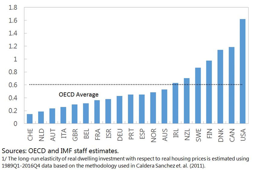
© 2018 International Monetary Fund                                                              WP/18/164

                                         IMF Working Paper

                                         European Department

                Fundamental Drivers of House Prices in Advanced Economies

                                       Prepared by Nan Geng1

                          Authorized for distribution by Craig Beaumont

                                                July 2018

    IMF Working Papers describe research in progress by the author(s) and are published to
    elicit comments and to encourage debate. The views expressed in IMF Working Papers are
    those of the author(s) and do not necessarily represent the views of the IMF, its Executive Board,
    or IMF management.

                                                Abstract

House prices in many advanced economies have risen substantially in recent decades. But
experience indicates that housing prices can diverge from their long-run equilibrium or
sustainable levels, potentially followed by adjustments that impact macroeconomic and
financial stability. Therefore there is a need to monitor house prices and assess whether
they are sustainable. This paper focuses on fundamentals expected to drive long-run trends
in house prices, including institutional and structural factors. The scale of potential
valuation gaps is gauged on the basis of a cross-country panel analysis of house prices in
20 OECD countries.

JEL Classification Numbers: C33, C51, E21, R21, R31

Keywords: Housing markets, House prices, Valuation gaps, OECD countries

Author’s E-Mail Address: ngeng@imf.org

1
  The author is grateful to Craig Beaumont for his helpful comments and suggestions. The paper has also
benefited from discussions with Jesper Lindé, Tom Dorsey, the Norwegian and Dutch authorities, and feedback
from seminar participants at the IMF and the Sveriges Riksbank. All remaining errors are my own.
3
Contents                                                                            Page
Abstract………………………………………………………………………………………..2
I. Introduction…………………………………………………………………………………4
II. Fundamental Determinants of House Prices……………………………………………….7
III. A Cross-Country Model of Trends in House Prices……………………………………..13
IV. Empirical Findings……………………………………………………………………….15
V. Conclusions……………………………………………………………………………….20

FIGURES
1. Uptrend in PTI and DTI Ratios in Selected Advanced Economies………………………...4
2. Real House Price Index…………………………………………………………………….4
3. Real House Price Index…………………………………………………………………….5
4. Household Debt…………………………………………………………………………….5
5. Price-to-Rent Ratio: United States…………………………………………………………6
6. House Prices and Per Capita Disposable Income…………………………………………..7
7. House Prices and Per Capita Financial Net Wealth………………………………………..8
8. House Prices and Population……………………………………………………………...9
9. PTI Ratios and Housing Supply Relative to Demographic Needs………………………..9
10. Low Supply Response to Rising Demand Can Amplify Price Increases………………..10
11. Estimated Long-Run Housing Supply Elasticity ...……………………………………...10
12. Recurrent Taxes on Residential Property………………………………………………..11
13. Tax Relief for Housing Finance, 2016…………………………………………………...12
14. Rent Control ...…………………………………………………………………………...13
15. Variation in Estimated Long-Run Impact of One Ppt Increase in Income on House
Prices……...………………………………………………………………………………….16
16. Variation in Estimated Long-Run Impact of One Ppt Increase in Real Mortgage Rate on
House Prices………………………………………………………………………………….16
17. Variation in Estimated Long-Run Impact of One Ppt Increase in Housing Stock Per
Capita on House Prices………………………………………………………………………17
18. Cross-Country variation in House Price Elasticities with Respect to Demand and Supply
Shifters……………………………………………………………………………………….17
19. Actual and Estimated Long-Run Equilibrium House Prices, and Estimated Valuation
Gaps in Selected OECD AEs………………………………………………………………...19
20. Housing Valuation Gap Under Different Model Specifications…………………………18

TABLES
1. Current MID from Personal Income Taxes and Recent Reforms in Selected AEs……….12
2. A Cross-Country Panel Model: Long-Run Determinants of Real House Prices………….15

ANNEX
I. Variable Definitions and Data Sources……………………………………………………24

References…………………………………………………………………………………...22
4
                                     I. INTRODUCTION

Over the past two decades, house prices have risen faster than income in many advanced
economies (AEs), leading to a strong uptrend in price-to-disposable income (PTI) ratios
(Figure 1). These large price increases have been associated with significant increases in
household debt, resulting in a similar rise in household debt-to-disposable income (DTI)
ratios.

                    Figure 1. Uptrend in PTI and DTI Ratios in Selected AEs

Within this broad uptrend, sizable reversals of housing prices have also arisen around the
global financial crisis (GFC), e.g., in Denmark, Ireland, and Spain, where prices have
recovered to some extent but have remained below their pre-crisis peaks (Figure 2). Such
reversals have had major macro-financial consequences, causing household deleveraging and
reduced consumption, and, in some cases, weakened financial intermediation.

                               Figure 2. Real House Price Index
                                         (1995 = 100)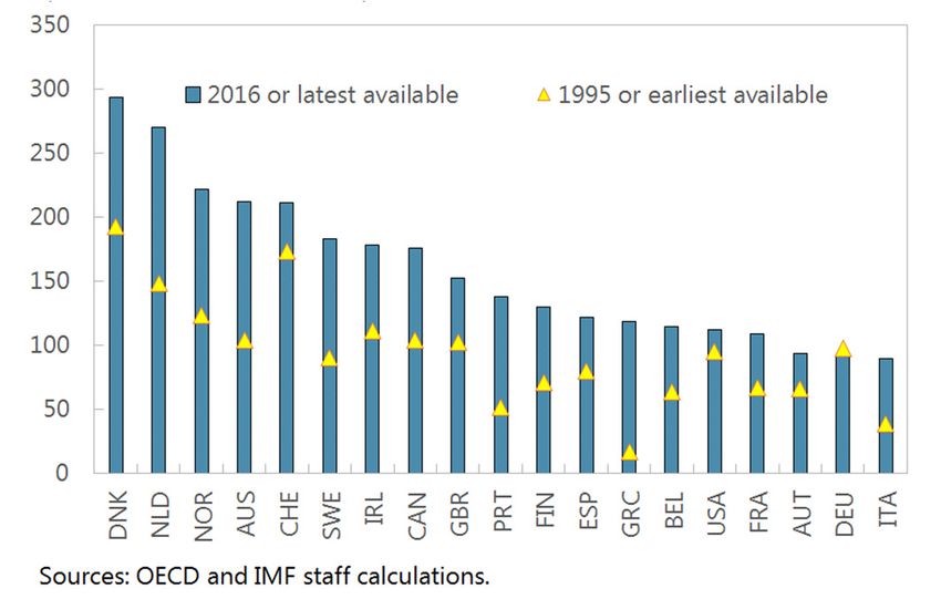
5
In contrast, some other AEs have experienced almost uninterrupted house price booms, with large
price rises even after the GFC, seen in house price inflation reaching double digits and price
levels and household debt ratios hitting record highs, e.g., in Sweden and Norway (Figure 3 & 4).

                               Figure 3. Real House Price Index
                                         (2010 = 100)

                                   Figure 4. Household Debt
                         (In percent of household net disposable income)

If increases in house prices become significantly disconnected from the fundamentals driving
the supply and demand for housing, the market is likely to become more vulnerable to a price
correction. This could pose significant risks to macroeconomic and financial stability through
the housing market’s impact on aggregate demand (i.e., residential construction and household
consumption) and on the banking sector (OECD, 2011; Mian et al., 2013; ECB, 2009).
Moreover, the high indebtedness that typically accompanies high housing prices tends to make
the economy more vulnerable to asset price movements, which can amplify shocks and
macroeconomic instability through the collateral channel (Hviid and Kuchler, 2017). Alongside
monitoring household debt, it is also important to monitor house prices and assess whether
housing valuations are sustainable.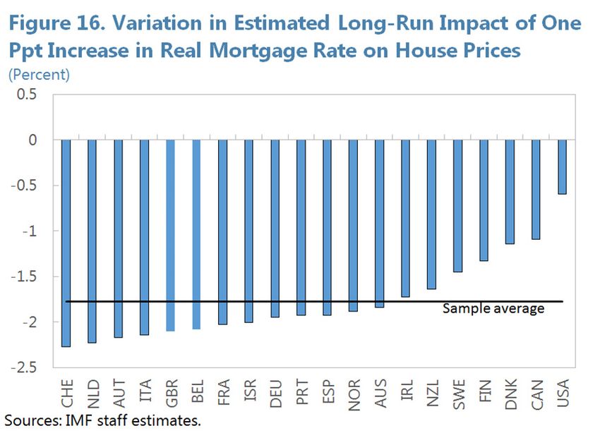
6
The most commonly used valuation benchmarks for house prices are long-run averages for
the PTI ratio and the price-to-rent (PTR) ratio. Despite being a useful metric for affordability,
the PTI ratio is not ideal for assessing the sustainability of housing valuations, because
deviations from historical averages may reflect fundamental drivers of house prices besides
income, e.g., interest rates. The PTR ratio compares house prices to the user cost of housing
(Poterba, 1992), which has the advantage of summarizing the impact of a range of
fundamentals while avoiding speculative factors. The PTR ratio appears quite informative for
markets like the U.S. (Figure 5), but doesn’t work well in countries where rental data don’t
reflect market costs due to rent controls e.g. Sweden, or a thin rental market e.g. Norway.

                              Figure 5. Price-to-Rent Ratio: United States
                                           (Index, 2010 = 100)

Another approach in the literature is to model housing prices using multivariate econometric
analysis—including factors such as disposable income, interest rates, demographics, and
supply factors influencing the available housing stock—and to use these models to estimate
the extent of any disequilibrium in housing prices. Girouard et al. (2006) and Turk (2015)
provide summaries of this work for AEs. While this approach reduces the risk of omitting
factors that determine sustainable house prices, the effects of policy changes related to
housing are not often captured.

This paper aims to assess housing valuation risks by modelling the sustainable levels of
house prices for 20 AEs in the OECD.2 A novel contribution of the paper is its focus on the
role of policy, institutional, and structural factors—i.e. tax incentives for home
ownership, rent controls, and the long-run supply responsiveness of housing construction—in
shaping long-run house price trends. Given the slow-moving nature of these factors,
modelling their impact requires a cross-country panel methodology. Hence the paper
provides estimates of the differential impact of policy and structural factors on house prices
across countries in addition to consistent estimates of valuation gaps for 20 AEs.

2
 The 20 countries included in the sample are Australia, Austria, Belgium, Canada, Denmark, Finland, France,
Germany, Ireland, Israel, Italy, the Netherlands, New Zealand, Norway, Portugal, Spain, Sweden, Switzerland,
United Kingdom, and United States.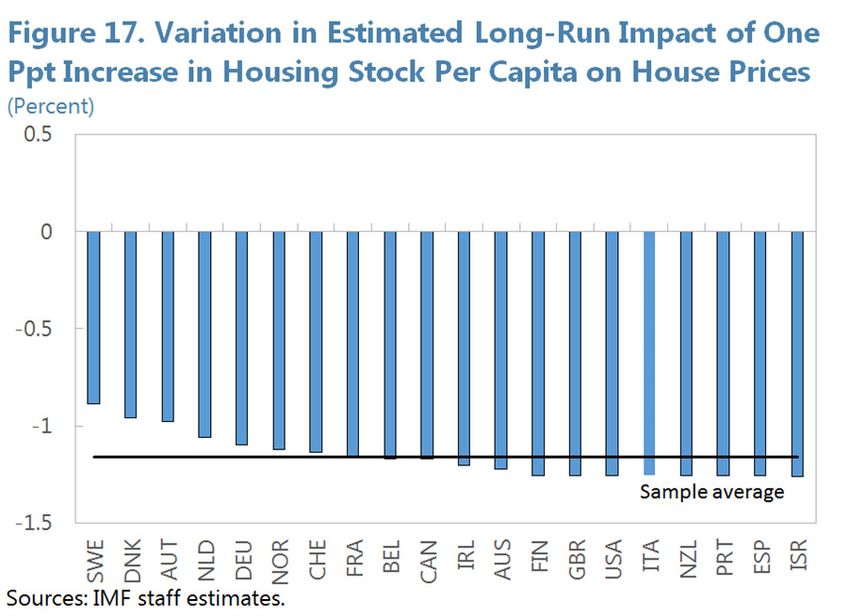
7
The paper is structured as follows. Section II discusses the driving forces behind the long run
uptrend in house prices, including demand, supply, institutional, and structural factors.
Section III lays out the cross-country model of long-run equilibrium housing prices, which
seeks to take into account policy, institutional, and structural factors. Section IV presents
estimation results using data from 20 OECD countries and discusses empirical findings.
Section V concludes.

                   II. FUNDAMENTAL DETERMINANTS OF HOUSE PRICES

Theoretical models, e.g., Skaarup and Bodker (2010), and the empirical literature on the
housing market, suggest that over the long-run house prices depend positively on disposable
income, wealth, and demographic needs, and negatively on user costs and the housing stock.
This section illustrates developments in these factors for the AEs. It also presents the data
developed for policy, institutional, and structural factors that can affect house price dynamics
through their influence on housing demand and supply, e.g., tax policies, rental market
regulations, and factors affecting housing supply such as land and building regulations.

Demand Factors

Household disposable income plays a key role in shaping house price trends. The higher
the real per-capita disposable income (RPDI) of households, the more they can spend to
purchase a house or service a mortgage, pushing up house prices. Average annual growth in
RPDI is positively correlated with that for house prices in our sample countries (Figure 6).
Interestingly, this bivariate relationship has a slope exceeding unity.

                    Figure 6. House Prices and Per Capita Disposable Income
                    (Average annual percent change from 1995: Q1 to 2016: Q4)

Household net financial wealth also appears to be a determining factor of house prices.
The accumulation of financial net wealth by households has exerted upward pressure on
housing demand and contributed to the rise in house prices (Figure 7). For example, Claussen
8
(2013) finds that of the rise in house prices in Sweden since the mid-1990s, about 60 percent
can be explained by the increase in real disposable income, while the rise in household real
financial wealth accounts for slightly under 10 percent of the increase.

                        Figure 7. House Prices and Per Capita Financial Net Wealth
                         (Average annual percent change from 1995: Q1 to 2016: Q4)

Housing demand has also been fueled by declining interest rates. Interest rates have gone
down substantially since 2000 and stayed low in recent years, with real rates falling close to
or below zero in many countries. These falls reduce the user cost of housing through savings
on financing costs. In addition, housing investment returns have held up as long-term bond
yields declined along with the slide of policy rates, which stimulated housing purchases for
investment purposes. From studies on advanced countries, the semi-elasticity of real housing
prices with respect to interest rates ranges between close to zero and 6 percent.3

Demographic trends reinforced the high demand for owner-occupied housing.
Population growth, including from high rates of net migration, together with increases in the
share of the population in the age group for household formation, will boost housing demand.
In many AEs—including Australia, Ireland, Israel, New Zealand, Norway—the fast growth
of population at household formation ages since the mid-1990s has been associated with
large increases in real house prices (Figure 8).

3
    See Turk (2015) for a summary of findings from the literature.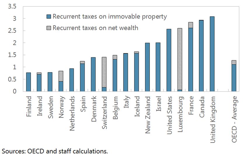
9
                             Figure 8. House Prices and Population
                    (Average annual percent change from 1995: Q1 to 2016: Q4)

Supply Factors

Undersupply conditions can also contribute to housing price gains outpacing incomes.
Over recent decades, residential investment has grown significantly in many countries, but it
remained below demographic needs and significant housing supply shortages accumulated in
some. For example, in Norway and Israel, lags in supply responses to demographic needs
have resulted in continued increases in the ratio of population to the stock of dwellings over
the past decade or more, associated with prices rising faster than incomes (Figure 9). In the
case of Sweden, a prolonged period of underinvestment in housing has been identified as a
key driver of Sweden’s house price inflation (IMF, 2016; European Commission, 2017).

            Figure 9. PTI Ratios and Housing Supply Relative to Demographic Needs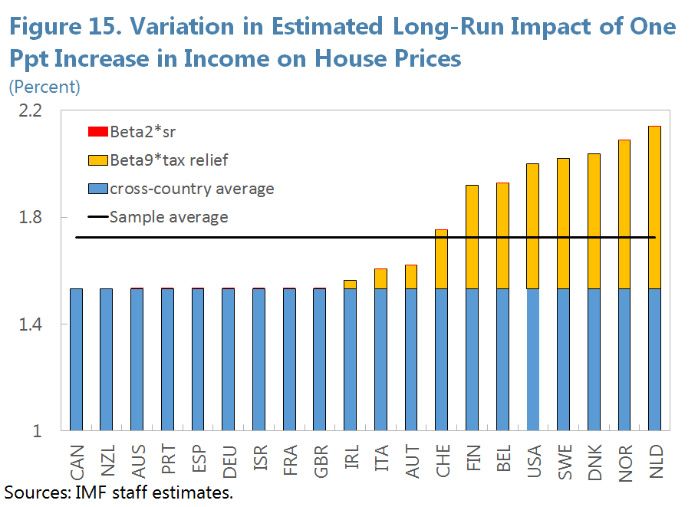
10
Structural and Institutional Factors

Differences in price elasticities of housing supply can affect house price dynamics.
Subject to a given increase in long-run demand, markets with an inelastic (steeper) long-run
supply curve will not build as much new dwellings as markets with elastic supply, resulting
in greater increase in prices (Figure 10; Anundsen et al., 2016). Divergences in housing
supply elasticities may reflect both natural (i.e. topographical) and man-made constraints
(e.g. stringent local regulations on land use, cumbersome building permit procedures, and
capacity constraints in the construction sector). To take these structural differences in the
supply side into account, long-run supply elasticities for each of the 20 OECD countries in
the sample are estimated separately using quarterly data for 1989-2016 based on the
methodology of Caldera Sanchez et. al. (2011) using a system of long-run price and
investment equations. The derived long-run price elasticities of new housing supply vary
greatly from about 0.2 in Switzerland to 1.6 in the US (Figure 11), indicating that it is
important to allow for differences in the slope of the long-run housing supply curve.

             Figure 10. Low Supply Response to Rising Demand Can Amplify Price Increases

                                                                                LRS
         P
                                Long-run (LR) S           P

                                                         ∆P

    ∆P

                                             LRD’                                             LRD’
                                       LRD                                              LRD

                                        Q                                                Q
                      Elastic market                                 Inelastic market

                     Figure 11. Estimated Long-Run Housing Supply Elasticity 1/
11
Tax incentives for mortgage financing and home ownership, which reduce the user cost
of housing, can contribute to high and rising house prices.4 In many AEs, housing
investment receives favorable tax treatment relative to other investment. This favorable tax
treatment on housing investment may crowd out capital from more productive use than
housing and encourage excessive leverage (OECD, 2009; Geng et al., 2016).
Typically, capital gains taxes are exempted, deferred, or reduced for principle residences
after a certain holding period, while such an exemption is usually not granted to other
types of investment (ESRB, 2015). In some cases, the economic importance of recurrent
property taxes is reduced by low tax rates and outdated or below-market cadastral values
(Figure 12; OECD, 2011).
Figure 12. Recurrent Taxes on Residential Property
(Percent of GDP; in 2015)
Many countries grant tax relief on mortgage interest payments, thereby incentivizing
households to borrow more and purchase more expensive houses (Andrews, 2010).
Mortgage interest deductibility (MID) is usually capped at a nominal amount, but is
unbounded in some cases, e.g., the Netherlands, Sweden, and Norway (Table 1). This
tax relief tends to be capitalized into house prices, without necessarily expanding
housing opportunities for households (Capozza et al., 1996; Harris, 2010). Several
countries have implemented reforms to gradually phase out or reduce MID in recent
years. For example, Portugal and Spain have removed MID since 2012 and 2013,5
respectively, and in Ireland from 2018. More gradual and/or moderate reductions of
MID have been adopted in Denmark, Finland, and the Netherlands. We have therefore
updated the 2009 tax relief index from the OECD to take these reforms into account.6
4
Key elements of user cost of owner-occupied housing include adjusted mortgage interest costs for tax
deductibility, maintenance costs, property taxes, and expected net capital gains (Poterba, 1984).
5
Loans taken out before end-2011 in Portugal, and before end-2012 in Spain, still enjoy MID in the form of a
tax credit at 15 percent of the interest payment up to a ceiling.
6
This OECD index takes into account if interest payments on mortgage debt are deductible from taxable
income, if there are any limits on the allowed period of deduction of the deductible amount, if tax credits for
loans are available, and if imputed rent from home ownership is taxed.12
According to this indicator, as of 2016 tax relief is most generous in the Netherlands and
effectively zero in countries where mortgage loans are not tax favored (Figure 13).
Table 1. Current MID from Personal Income Taxes and Recent Reforms in Selected AEs
Denmark Finland Ireland Netherlands Norway Spain Sweden UK
Rate of 32.7 35 for capital income Removed from 100 percent for pre- 100 (full 0 for 30 0
deductibility deduction 2018 (Until 2017: 2013 loans; 100 deduction) properties deduction
(in percent) Up to 30 percent percent for post- purchased against tax
for first-time 2013 fully after Jan 1, liabilities
homebuyers, and amortizing loans 2013
up to 15 percent for (within 30 years)
others.)
Caps/notes/r Reduced from Reduced from 65 Deductibility varies The maximum tax 15 percent Reduced to Mortgage
ecent reforms 32.7 percent in percent in 2016 to 25 by origination date rate at which deduction up 21 percent interest
2012 to 25 percent in 2019; 30 (only 2004-12), and mortgage interest to EUR 9,040 for annual relief at
percent in 2019 percent for the excess borrower's marital can be deducted per year, for mortgage source
(27 percent in interest expense over status has been reduced properties interest abolished
2017) for capital income by 0.5 points per purchased expense in 2000
annual against income tax, year from 52 before Dec 31, over SEK
mortgage up to EUR 1,400 per percent in 2013, to 2012 100,000
interest year (32 percent for 38 percent in 2041
expense over first-time (49.5 percent in
DKK 50,000 homebuyers) 2018) 1/
Sources: National tax and other authorities; Bourassa et al. (2013); Smidova (2016).
1/ The recently released coalition agreement proposes a much more rapid phase-out in steps of 3 percentage points annually until the basic rate of
37 percent is reached in 2023, but this is still subject to approval by the parliament.
Figure 13. Tax Relief for Housing Finance, 2016
(Index; increasing in degree of tax relief)
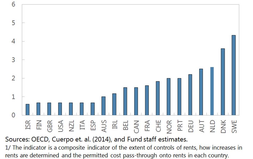
Rent controls, by reducing incentives to use housing efficiently, tend to raise house
prices. The option to rent housing provides a potential check on house price pressures. Rent
controls, however, can create “lock-in” effects where renters remain in space that may
exceed their needs, reducing the effective housing supply and creating queues that make
renting a less viable alternative. We have therefore updated the 2009 rent control index from
the OECD taking into account recent reforms, e.g., the 2013 reform in Spain (Figure 14).13
According to this indicator, Sweden currently has the most stringent rent controls among
OECD countries, which has resulted in a declining supply of rental apartments as they are
converted into tenant-owned condominiums. Waiting times for rental apartments average at
10 years, leaving many households with no option but to purchase housing, which is also
incentivized by the generous tax deductibility of mortgage interest payments (IMF, 2017).
Figure 14. Rent Control 1/
(Scale 0–6, increasing in degree of control)
III. A CROSS-COUNTRY MODEL OF TRENDS IN HOUSE PRICES
The long-run relationship between real house prices and their potential determinants
discussed above is modelled in a cross-country setting. Following the literature on
modelling the housing market,7 housing demand (D) can be expressed as a function of the
real price level of housing ( ) and other factors shifting demand (summarized in ). In the
long run, the equilibrium price of housing ( ∗ ) is that at which the demand for housing
matches the stock of housing ( ):
∗
, (1)
With households maximizing an inter-temporal utility function with non-separability
between housing and non-housing consumption (Skaarup and Bodker (2010)), the long-run
housing price ( ∗ ) can be derived as a reduced form of its fundamental determinants, which
include real per capita household disposable income , user cost of housing ,
real per capita household net financial wealth , and the housing stock per capita . 8
7
See Meen (2001), Aoki et al. (2002), and Poterba (1984), etc.
8
The aim of this paper is not to achieve the best fitting model of house prices, but to account for their long-run
trends with factors that are not highly dependent on housing prices, as a basis for estimating the sustainable
level of house prices. Credit is not included in the model because it can be driven by house prices; higher house
prices increase the debt needed to purchase housing while also expanding the value of collateral for borrowing.14
∗
, , , (2)
In practice, actual house prices will not always be at the long-run equilibrium, such that for
each country i, and time t, there is an error term between the observed price and the
∗
long-run equilibrium real house prices which gives the following formula for :
∗
, , , (3)
In the estimated equation, the user cost would ideally be captured by the real after-tax interest
rate for mortgage borrowing. In practice, for most countries it is difficult to calculate the
effective after-tax interest rate, so we use the updated version of tax relief index from the
OECD (discussed in Section II) to proxy for the generosity of tax incentives for home
ownership and mortgage financing. The value of tax incentives for housing will tend to rise
with household income, which is captured by including an interaction term between tax relief
and income, although the level of debt may also shape the value of this relief. A square term
of the real mortgage rate is also added to capture any non-linear relationship between house
prices and interest rates following the present value formula.
In addition, the updated OECD rent control index (discussed in Section II; rescaled to
0-1) is added to test the impact of rent control, by interacting it with housing supply as it
is expected to hinder the efficient use of existing housing stock. To test whether the long-run
impact of demand factors depends on the elasticity of housing supply, we include additional
interaction terms of the demeaned long-run supply elasticities with demand variables in
the full augmented model. Therefore, the total long-run impact of demand factors can vary
across countries. In summary, the long-run relationship between real house prices and their
potential determinants is estimated in a cross-country panel model as follows:
∗ ∗ ∗
∗ ∗ (4)
The error term, which is used to gauge the extent of possible housing valuation gaps, is
expected to be stationary, i.e., equation (4) is a cointegrating relationship. Country fixed
effects are included to reflect unobserved cross-country differences affecting price levels.
Annex I summarizes the definition of variables and data sources. All variables are in log
terms except for mortgage rates, the housing stock to population ratio, the tax relief and rent
control indices, and long-run supply elasticities. In addition, robust standard errors are
clustered at the country level to allow for an arbitrary variance-covariance matrix within each
country. The estimation sample includes 2042 observations for 20 advanced countries in the
OECD over the period of 1990: Q3–2016: Q4.15
IV. EMPIRICAL FINDINGS
The estimation results on long-run determinants of real house prices under different
model specifications are presented in Table 2. Column (2) is the baseline and columns
(3–5) show results under augmented model specifications that take into account policy,
institutional, and structural factors. The explanatory variables all have the expected sign and
most are statistically significant. The residuals are confirmed to be stationary, i.e., equation
(4) is a cointegrating relationship.
Table 2. A Cross-Country Panel Model: Long-Run Determinants of Real House Prices
Variables (1) (2) (3) (4) (5)
y , log 1.652 1.638 1.538 1.544 1.533
[0.034]*** [0.034]*** [0.036]*** [0.036]*** [0.037]***
morr , percent ‐1.922 ‐2.759 ‐2.234 ‐2.116 ‐1.776
[0.214]*** [0.431]*** [0.431]*** [0.432]*** [0.426]***
morr^2 , percent 0.079 0.066 0.051 0.058
[0.035]** [0.034]** [0.033] [0.032]*
w , log 0.031 0.033 0.023 0.020 0.056
[0.008]*** [0.009]*** [0.009]** [0.009]** [0.010]**
s, percent ‐1.070 ‐1.080 ‐0.943 ‐1.267 ‐1.322
[0.062]*** [0.062]*** [0.063]*** [0.103]*** [0.102]***
tr * y (log) 0.362 0.351 0.487
[0.048]*** [0.047]*** [0.046]***
rc * s (percent) 1.156 0.436
[0.294]*** [0.230]*
sr * y (log) ‐0.007
[0.141]
sr * morr 1.133
[0.154]***
sr *w (log) ‐0.060
[0.033]*
Obervations 2042 2042 2042 2042 2042
Adj. R‐squared 0.853 0.853 0.856 0.857 0.867
Number of countries 20 20 20 20 20
Country fixed‐effect Y Y Y Y Y
Corrected for heteroskedasticity Y Y Y Y Y
Panel Cointegration Tests for Model (5)
Kao (Engle‐Granger based) t‐Statistics ‐3.806 Prob. 0.0001
Panel Unit Root Test on Residuals of Model (5)
Levin, Lin & chu t Statistics ‐2.705 Prob. 0.003
Note: Dependent is the log of real house prices. Significance at 1, 5, and 10 percent levels indicated by ***, **, and *, respectively.
Robust standard errors clustered at the country level.
The estimated long-run impact of fundamental demand and supply factors are
consistent with priors and statistically significant. On the demand side, a 1 percent rise in
per capita disposable income raises long-run equilibrium house prices by a cross-country
average of 1.5–1.7 percent, suggesting that housing is a luxury good, accounting for much of16
the uptrend in PTI ratios.9 Meanwhile, a 1 percentage point increase in the real mortgage rate
reduces real house prices by a cross-country average of about 1.8–2.8 percent. In addition,
real per capita household net financial wealth has a small positive impact on real house
prices. On the supply side, a 1 percent increase in the housing stock per capita is associated
with a reduction in house prices by about 1.3 percent in countries with no rent control.
The impact of demand and supply factors on long-run house prices varies across
countries depending on policy and structural factors:
Depending on the generosity of tax
relief (and the long-run supply
elasticities), a 1 percent increase in per
capita disposable income results in
different impacts on house prices
across countries, with the largest
impact of 2.1 percent seen in the
Netherlands and the least impact of
1.6 percent seen in countries where
housing finance is not tax favored,
such as Canada (Figure 15).
With varying long-run supply
elasticities, the same increase in
mortgage rates can have significantly
different long-run impacts on house
prices across countries, with an
amplified impact seen in less elastic
markets (e.g., Switzerland) and a
moderated impact seen in more elastic
markets, e.g. the US (Figure 16).
As expected, rent controls are found to
offset part of the dampening effects of
supply increases on real house prices,
confirming that controls hinder the
efficient use of the housing stock. This
efficiency impact is concentrated on
countries with the most stringent
controls (Figure 17). In the case of
Sweden, which has the most stringent
rent control in our sample, a 1 percent
9
Our estimates are consistent with findings by studies for AEs, as summarized by Girouard et al. (2006). In
addition, more recent studies find a similar magnitude of this parameter, e.g. 1-1.3 as estimated by Andrews
(2010) for 15 OECD countries and 1.3 as estimated by Turk (2015) for Sweden.17
increase in the housing stock per capita reduces long-run house prices by only
0.9 percent compared with 1.3 percent in countries without rent control.
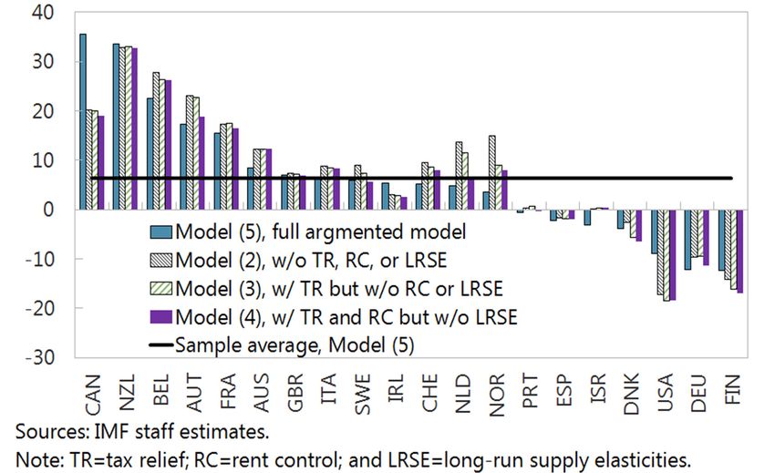
In summary, the estimation results confirm that policies and structural factors play an
important role in shaping long-run house price developments (Figure 18). Tax relief on
housing investment contributes to spurring housing demand and driving up house prices,
with a positive income shock translating into a greater price impact in countries with more
generous tax relief. For example, phasing out tax relief on mortgage financing and rent
controls in Sweden is estimated to help reduce house prices by about 4 percent in the long
run. Meanwhile, the long-run responsiveness of supply seems to primarily affect house price
elasticities with respect to mortgage rate, with larger long-run impact on real house prices in
markets with less elastic supply. In addition, rent control reduces the impact of supply
increases on house prices, but the impact is more moderate.
Figure 18. Cross-Country Variation in House Price
Elasticities with Respect to Demand and Supply Shifters
(Percent)
Country-by-country results are presented for augmented model estimates in column (5).
The long-run relationship broadly captures trends in housing prices since the early 1990s in
most countries (Figure 19). 10 The model suggests that overvaluation was widespread in the
years leading up to the GFC. In some countries, the fall in house prices after the GFC is
estimated to have put the market into undervaluation territory. Among those countries, house
prices have recovered thereafter, and as of end-2016 can be grouped as: (i) those estimated to
remain undervalued (Denmark, Finland, Germany, and the US); (ii) those estimated as
broadly fairly-valued (Ireland, Israel, Portugal, and Spain); and (iii) those back into
overvaluation territory (Australia, Austria, the Netherlands, and New Zealand).11 Meanwhile,
some other countries experienced limited housing price corrections after the GFC and are
10
For Belgium, France, and Germany, the gaps between the estimated long-run equilibrium and actual housing
prices are sizable for prolonged periods, as further discussed below.
11
The grouping of countries here is based on similarities in empirical results, and is not definitive.18
either: (i) estimated to be overvalued as of end-2016 (Canada, Norway, Sweden, and the
United Kingdom); or (ii) experiencing persistent overvaluation (Belgium, France, Italy,
Switzerland).12
The model estimation suggests on average a modest overvaluation of 6 percent on
current fundamentals including policy and structural factors. As illustrated in Figure 20,
in most cases the valuation gaps are similar across model specifications. For model (5),
estimated housing valuation gaps as of 2016: Q4 range from 12 percent undervaluation in
Finland to 35 percent overvaluation in Canada. However, real mortgage rates are well below
their average since 2000 so they may unwind to some extent over time. This would lower
equilibrium housing prices, implying that house prices could be more overvalued than
estimated if allowing for a normalization of interest rates. For example, based on our model
estimates, a 2 percentage point increase in the real mortgage rate would reduce house prices
by about 4–6 percent in equilibrium, implying that house prices could be up to 12 percent
overvalued on average in our sample countries.
Figure 20. Housing Valuation Gap Under Different Model Specifications
(Percent, as of 2016: Q4)
12
While our model points to a positive valuation gap—which has been shrinking since 2012 as household
disposable income recovers—for Italy, the Italian central bank’s housing model—which takes into account also
lending conditions—finds that house prices in Italy have remained in line with fundamentals during both the
GFC and sovereign debt crisis.Figure 19. Actual and Estimated Long-Run Equilibrium House Prices, and Estimated Valuation Gaps in Selected OECD AEs
Australia Austria Belgium Canada Denmark
30 40 40 40 60
30
20 2.4 30 40
20 20
10 2.2 20
10 20
2.0 2.8
2.8 0 0 2.0 0
0
2.2 10
-10 -10 1.8 2.4
2.4 2.0 -20
-20 -20 1.6 0
1.8 1.6
-20 2.0
2.0
1.6 -40
1.4
-40 -10 1.6
1.6 1.4
1.2 1.2
1.2 -20
1.2 1.2
1.0
1.0
0.8 0.8 0.8 0.8 0.8
90 92 94 96 98 00 02 04 06 08 10 12 14 16 90 92 94 96 98 00 02 04 06 08 10 12 14 16 90 92 94 96 98 00 02 04 06 08 10 12 14 16 90 92 94 96 98 00 02 04 06 08 10 12 14 16 90 92 94 96 98 00 02 04 06 08 10 12 14 16
Finland France Germany Ireland Israel
40 30 40 20 40
30 30
20
20 10 20
20
10
10
2.0 10
0 0
0 0 3.5 2.8
0
-10 1.8 1.3
1.2 -10 -10 3.0 -10 -20
2.4
-20 1.6 1.2
-20 -20 2.5
1.0 1.1 2.0 -40
1.4 -20
-30 2.0
1.0
0.8 1.6
1.2 1.5
0.9
0.6 1.0 1.2
0.8 1.0
0.4 0.8 0.7 0.5 0.8
90 92 94 96 98 00 02 04 06 08 10 12 14 16 90 92 94 96 98 00 02 04 06 08 10 12 14 16 90 92 94 96 98 00 02 04 06 08 10 12 14 16 90 92 94 96 98 00 02 04 06 08 10 12 14 16 90 92 94 96 98 00 02 04 06 08 10 12 14 16
19
Italy Netherlands New Zealand Norway Portugal
30 30 40 40 60
20 20 30
40
3.5 20
10 10 20
20
10
0 0 3.0
2.8 0 0
1.3 -10 -10 0 1.2
2.5 3.0 -10 -20
1.2 2.4
-20 1.1
-20 -20
2.5
1.1 2.0 1.0 -40
-30 2.0 -20
-30
2.0
1.0 0.9
1.6 1.5
0.9 1.5 0.8
-40
1.2 1.0
0.8 1.0 0.7
0.7 0.8 0.5 0.5 0.6
90 92 94 96 98 00 02 04 06 08 10 12 14 16 90 92 94 96 98 00 02 04 06 08 10 12 14 16 90 92 94 96 98 00 02 04 06 08 10 12 14 16 90 92 94 96 98 00 02 04 06 08 10 12 14 16 90 92 94 96 98 00 02 04 06 08 10 12 14 16
Spain Sweden Switzerland United Kingdom USA
30 40 40 60 40
20 30 30
40 20
20 20
10
2.4 20
10 10 2.4 0
0 1.0
2.4 0 0 1.6
2.0 0 -20
2.0
-10 -10 0.9
2.0 -10 1.4
1.6 -20
-20 -20 -40
1.6 1.6 0.8 -20
1.2
-30 1.2 -40
1.2 0.7 1.0
1.2
0.8 0.6 0.8
0.8
0.8 0.4 0.5 0.4 0.6
90 92 94 96 98 00 02 04 06 08 10 12 14 16 90 92 94 96 98 00 02 04 06 08 10 12 14 16 90 92 94 96 98 00 02 04 06 08 10 12 14 16 90 92 94 96 98 00 02 04 06 08 10 12 14 16 90 92 94 96 98 00 02 04 06 08 10 12 14 16
Note: Blue and red lines represent actual and estimated long-run equilibrium house prices, respectively; and green lines (RHS) refer to valuation gaps in percent.20
The estimated valuations from this exercise should be interpreted with caution. As for
any econometric analysis, the estimated equilibrium price levels are subject to uncertainty.
Moreover, for several countries, i.e., Belgium, France, and Germany, the estimated gaps
seem prolonged with actual prices only crossing equilibrium levels once. Although the case
of the Netherlands indicates that it is possible for prolonged gaps to eventually be corrected,
it may be that housing markets in these countries have some characteristics that are not fully
captured by the model, suggesting additional caution be taken when interpreting the results.13
In addition, any valuation at the country level risks concealing highly heterogeneous
valuation developments at the regional level.14
V. CONCLUSIONS
Assessing the sustainability of house price developments has become an integral part of
macro-financial surveillance. Many AEs have experienced a remarkable run-up in their
national housing markets in the past two decades and in some cases house prices have
remained strong in recent years. Understanding housing price developments and monitoring
the extent to which house prices deviate from levels supported by long-run fundamental
factors are important for assessing risks to financial and macroeconomic stability.
This paper models house prices on a cross-country basis seeking insights on deviations
from sustainable valuations. Based on standard theory, it selects a small set of supply and
demand fundamental drivers of house prices to model long-run equilibrium house prices in
20 AEs in the OECD. The novel feature of the model is the incorporation of policy,
institutional, and structural factors—i.e. tax incentives for home ownership, rent controls, and
the long-run supply responsiveness of housing construction. The estimated long-run
relationship broadly captures trends in housing prices since the early 1990s. Hence, the
uptrend in real housing prices largely reflects fundamentals, especially rising real disposable
incomes. On average, the overvaluation of housing prices on current fundamentals is modest,
but there are significant variations in the estimated valuation gaps across our sample.
Policy, institutional, and structural factors are found to be important determinants of
long-run equilibrium house prices. The impact of shocks to the traditional demand and
13
For example, the Belgian central bank’s housing model and the Selected Issues paper of the 2015 Article IV
Consultation with Belgium—which take into account a number of structural and financial factors such as the
reduction in household size and tax policy changes—find that house prices in Belgium were close to
equilibrium in the years following the GFC and have become overvalued only in the most recent years (by
11 percent at peak in 2015 and by 6.5 percent on average in 2017).
14
For example, while the overall long-run supply elasticity is high in Canada, Toronto and Vancouver have
much lower supply elasticities than the rest of Canada. With aggregate overvaluation being driven by Toronto
and Vancouver, model (5) may have overestimated the valuation gap. In this case, it may be that model (4)—
which does not include long-run elasticity of supply—provides a more accurate estimate, as it is also in line
with findings of the Bank of Canada.21 supply factors on long-run house prices varies significantly across countries depending on policies and structural factors. In particular, more generous tax relief, stricter rent control, and below-average long-run supply responsiveness are found to drive up house prices. In this regard, structural reforms in the housing market should be considered alongside macroprudential instruments. Structural reforms can over time improve housing affordability, thereby reducing debt accumulation and enhancing financial stability. These structural reforms include, but are not limited to, reforms to raise the long-run elasticity of housing supply, phasing out rent control, and reducing tax incentives for home ownership and debt financing. Such instruments may complement and support the more commonly used macroprudential tools such as limits on loan-to-value ratios, as the impact of reforms on supply and demand fundamentals may shape longer-term expectations in the housing market.
22

                                        References

Andrews, D., 2010, “Real House Prices in OECD Countries: The Role of Demand Shocks
      and Structural and Policy Factors,” OECD Economics Department Working Papers
      No. 831.
Andrews, D., A. Caldera Sánchez and A. Johansson, 2011, “Housing Markets and Structural
      Policies in OECD Countries”, OECD Economics Department Working Papers,
      No. 836.
Anundsen, A.K. and C. Heebøll, 2016, “Supply Restrictions, Subprime Lending and
      Regional US House Prices,” Journal of Housing Economics, 31: pp. 54–72.
Aoki, K., Proudmand, J., Vlieghe, G., 2002, “House Prices, Consumption and Monetary
       Policy: A Financial Accelerator Approach,” Mimeo, Bank of England, Presented at
       the 2002 CEPR European Summer Symposium in Macroeconomics.
Bourassa, S., Haurin, D., Hendershott, P., and Hoesli, M., 2013, “Mortgage Interest
      Deductions and Homeownership: An International Survey,” Journal of Real Estate
      Literature, 2013, Vol. 21, No. 2, pp. 181–203.
Caldera Sanchez and Johansson, 2011, “The Price Responsiveness of Housing Supply in
       OECD Countries,” OECD Economics Department Working Papers No. 837.
Capozza, D., R. Green and P. Hendershott, 1996, “Taxes, Mortgage Borrowing, and
      Residential Land Prices,” Economic Effects of Federal Tax Reform, ed. H.J. Aaron
      and W.G. Gale, Brookings Institution Press, Washington, pp. 171–198.
Claussen, C. A., 2013, “An Error-Correction Model of Swedish House Prices,” International
       Journal of Housing Markets and Analysis 6(2), pp. 180–196.
Cuerpo, C., Kalantaryan, S. and Pontuch, P., 2014, “Rental Market Regulation in the
      European Union,” European Commission Economic Papers 515, 2014.
Dermani, Emilio, Jesper Lindé, and Karl Walentin, 2016, “Is a bubble forming in Swedish
      housing prices?” Sveriges Riksbank Economic Review 2016:2.
ECB, 2009, “Housing Finance and Monetary Policy,” Working Paper Series No. 1069.
European Commission, 2017, “Country Report Sweden 2017,” Commission Staff Working
      Document 2017 92 final.
European Systemic Risk Board (ESRB), 2015, Report on Residential Real Estate and
      Financial Stability in the EU, December 2015.
Geng, Nan and N. Arnold, 2016, “The Housing Boom and Macroprudential Policy,” Norway
      Selected Issues, IMF Country Report No. 16/215.
23
Geng, Nan, 2017, “Are House Prices Overvalued in Norway?—A Cross-Country Analysis,”
Norway 2017 Selected Issues, IMF Country Report No. 17/181.
Girouard, N., M. Kennedy M., P. van den Noord P. and C. André (2006), “Recent house
price developments: the role of fundamentals,” OECD Economics Department
Working Papers No. 475.
Green, R. K., S. Malpezzi and S.K. Mayo, 2005, “Metropolitan-Specific Estimates of the
Price Elasticity of Supply of Housing and Their Sources,” American Economic
Review 95 (2): pp.334–339.
Harris, B., 2010, “The Effect of Proposed Tax Reforms on Metropolitan Housing Prices,”
Tax Policy Center Working Paper, April.
Hviid, S. and Kuchler, A., 2017, “Consumption and Savings in A Low Interest-Rate
Environment,” Working Paper No. 116, Danmarks Nationalbank.
International Monetary Fund (IMF), 2016, Sweden: Staff Report for the 2016 Article IV
Consultation, IMF Country Report No. 16/353, 2016.
International Monetary Fund (IMF), 2017, Sweden: Staff Report for the 2017 Article IV
Consultation, IMF Country Report No. 17/350, 2017.
Meen, G., 2001, “The Time-Series Behavior of House Prices: A Transatlantic Divide?”
Journal of Housing Economics 11 (1), pp. 1–23.
Mian, A., K. Rao, and A. Sufi, 2013, “Household Balance Sheets, Consumption, and the
Economic Slump,” The Quarterly Journal of Economics 128 (4), 1687–1726.
OECD, 2009, “Taxation and Growth,” Chapter 5, Going for Growth 2009 (Paris: OECD).
OECD, 2011, “Housing and the Economy: Policies for Renovation,” Chapter 4 in Economic
Policy Reforms 2011: Going for Growth (Paris: OECD).
Poterba, J., 1984, “Tax Subsidies to Owner-Occupied Housing: An Asset Market Approach,”
Quarterly Journal of Economics 99, pp. 729–752.
Poterba, J., 1992, “Taxation and Housing: Old Questions, New Answers,” American
Economic Review, 82 (2): 237–242.
Skaarup, M. and Bodker, S., 2010, “House Prices in Denmark: Are They Far From
Equilibrium?” Denmark Finanministeriet Working Paper 21/2010.
Smidova, Z., 2016, “Betting the House in Denmark,” OECD Economics Department
Working Paper No. 1337.
The Dutch Government, 2017, “Confidence in the Future: 2017–2021 Coalition Agreement.”
Turk, R., 2015, “Housing Price and Household Debt Interactions in Sweden,” IMF Working
Paper 15/276, 2015.24
Annex I: Variable Definitions and Data Sources
Variable Definition / Note Source
Real house price index, in log terms, OECD.
seasonally adjusted
Real per capita household personal Haver Analytics, national
disposable income, in log terms, seasonally statistics websites.
adjusted.
Real mortgage rate, in percent. Calculated as Haver Analytics, national
weighted nominal mortgage rate (all statistics websites.
maturities) minus the HICP inflation rate.
Real per capita household net financial OECD, Haver Analytics,
wealth, in log terms. and national statistics
websites. Quarterly data is
generated by interpolating
annual data using a cubic
spline.
Housing stock per capita, ratio. OECD, Haver Analytics,
national statistics websites,
and country authorities.
Index of tax relief on housing finance. The OECD, ESRB (2015), IMF
indicator takes into account whether interest country staff reports,
payments on mortgage debt are deductible country authorities, and
from taxable income, if there are any limits Fund staff calculations.
on the allowed period of deduction or the
deductible amount, if tax credits for loans
are available, and if imputed rent from home
ownership is taxed.
Index of the strictness of rent controls. A OECD, Cuerpo et. al.
composite indicator of the extent of controls (2014), IMF country staff
on rents, how increases in reports, and Fund staff
rents are determined, and the permitted calculations.
pass-through of cost into rents in each
country.
Long-run elasticity of real dwelling Estimated using
investment with respect to real housing 1989: Q1–2016: Q4 data
prices. based on the methodology
used in Caldera Sanchez et.
al. (2011).You can also read