How Much Do Households Dislike Local Density? And Do Developers Fully Consider Their Preferences? Evidence from a Policy Change in Singapore ...
←
→
Page content transcription
If your browser does not render page correctly, please read the page content below
DISCUSSION PAPER SERIES

IZA DP No. 14730

How Much Do Households Dislike Local
Density? And Do Developers Fully
Consider Their Preferences? Evidence
from a Policy Change in Singapore
Eric Fesselmeyer
Haoming Liu
Louisa Poco

SEPTEMBER 2021
DISCUSSION PAPER SERIES

IZA DP No. 14730

How Much Do Households Dislike Local
Density? And Do Developers Fully
Consider Their Preferences? Evidence
from a Policy Change in Singapore
Eric Fesselmeyer
Monmouth University
Haoming Liu
National University of Singapore and IZA
Louisa Poco
National University of Singapore

SEPTEMBER 2021

Any opinions expressed in this paper are those of the author(s) and not those of IZA. Research published in this series may
include views on policy, but IZA takes no institutional policy positions. The IZA research network is committed to the IZA
Guiding Principles of Research Integrity.
The IZA Institute of Labor Economics is an independent economic research institute that conducts research in labor economics
and offers evidence-based policy advice on labor market issues. Supported by the Deutsche Post Foundation, IZA runs the
world’s largest network of economists, whose research aims to provide answers to the global labor market challenges of our
time. Our key objective is to build bridges between academic research, policymakers and society.
IZA Discussion Papers often represent preliminary work and are circulated to encourage discussion. Citation of such a paper
should account for its provisional character. A revised version may be available directly from the author.

                                                     ISSN: 2365-9793

                                           IZA – Institute of Labor Economics
Schaumburg-Lippe-Straße 5–9                      Phone: +49-228-3894-0
53113 Bonn, Germany                             Email: publications@iza.org                                    www.iza.org
IZA DP No. 14730 SEPTEMBER 2021
ABSTRACT
How Much Do Households Dislike Local
Density? And Do Developers Fully
Consider Their Preferences? Evidence
from a Policy Change in Singapore
This paper measures how much households dislike density in their immediate surroundings.
Using transaction and administrative data in Singapore, and exploiting the introduction of
a regulation that restricted the number of housing units for certain land lots, we find that
households do indeed discount density: a 10% increase in within-development density
decreases price per square meter by up to 4%. Further, we find that the mean price per
square meter of the average development increased by 1 to 3% after the regulation was
introduced, while the amount of built-up space remained constant. The increase in total
revenue suggests that developers may underestimate the externality caused by density.
Our results are particularly relevant during the lockdowns and social distancing of the
coronavirus pandemic.
JEL Classification: R20, R21, R38
Keywords: density, regulation, land-use policy, externalities
Corresponding author:
Haoming Liu
Department of Economics National
University of Singapore
1 Arts Link
Singapore 117570
E-mail: ecsliuhm@nus.edu.sg1 Introduction
As the world continues to urbanize, cities have become more dense, leading to externalities such
as traffic congestion, air pollution, and loss of open spaces. In response, land-use regulations have
become widespread as cities attempt to control the intensity of residential development and strike
a balance between fully utilizing land and ensuring livability.
An extensive literature has explored land-use restrictions (Gyourko and Molloy, 2015; Molloy,
2020), finding that such regulation leads to a smaller stock of housing and higher prices in the United
States (Glaeser and Gyourko, 2018; Zabel and Dalton, 2011; Ihlanfeldt, 2007) and internationally
(Hilber and Vermeulen, 2016; Tan et al., 2020). There are fewer papers that focus on the economic
effects of density itself, with Ahlfeldt and Pietrostefani (2019), Ahlfeldt et al. (2015), Ciccone and
Hall (1996), and Brueckner and Largey (2008) being some prominent examples, and even fewer
papers that consider how local density, that is, the density of the immediate surroundings, affects
households, which is the focus of this paper.1
Local density is particularly relevant during the coronavirus pandemic, since it has highlighted
the value of space as we work and spend much of our time at and near our homes during lockdowns
and social distancing. Indeed, early speculation that denser cities would experience more infections
has been refined to emphasize the importance of crowdedness of the immediate environment, for
instance, at home, in dormitories, in offices, and on public transportation (Fang and Wahba, 2020;
Zhong and Teirlinck, 2020). The pandemic has also underscored inequalities in living conditions as
poorer and more crowded neighborhoods often suffer more than predominantly wealthier and less
populated ones (Arango, 2021), and well-to-do city dwellers are more likely to move to suburban
or rural locations (Lerner, 2020). Neuroscientists and psychologists even propose that people are
learning new emotional experiences during the pandemic: unease around strangers and aversion to
crowds (Kiefer, 2020).
In addition to the risk of infectious disease and its associated effects in the new pandemic
world, drawing on findings in psychology and sociology we speculate that households dislike local
density because of a range of other factors including competition for facilities and common areas,
1
Tang and Yiu (2010) and Lee (2016) concluded that buyers pay more when there is more space and less density
locally but did not address the endogeneity of density.
1lack of privacy, noise, poor sleep, and adverse social interactions that cause stress, conflict, and
pathological behavior, which have been found to be more common in crowded areas (Gray, 2001;
Gómez-Jacinto and Hombrados-Mendieta, 2002; Chan, 1999).
To summarize succinctly, local density has a deep, continual impact on our physical and mental
well-being but there is little economic research that has attempted to measure people’s disutility to
it. One sensible approach is to measure how much less housing costs in more dense environments,
the approach we take in our research. Providing policymakers with an accurate measure of the
discount people place on dense living environments will allow more efficient planning and zoning
policies, particularly if policymakers are less aware of the impact of local density compared to other
more well-known externalities.
To measure how much households value less density, we constructed a novel dataset from
planning documents of relatively low-density residential developments in Singapore and combined it
with transaction data.2 We find that households do place a premium on less crowded environments:
a 10% increase in density reduces the price per square meter by up to 4%. To the best of our
knowledge our findings are the first to measure the causal effect of local density on prices in
relatively low-density developments.3
Our measure of density is the number of housing units per meter of lot size, which one would
expect to be endogenous in a price regression. For instance, density would be endogenous if
developers build more intensely in especially attractive areas. To address such endogeneity we
make use of a first-of-its-kind regulation in Singapore introduced in November 2011 in response to
developers building an increasing number of very small housing units, also known as “shoebox”
units.4
The regulation imposed a minimum average size of housing units in developments built on lots
with a 1.4 Floor Area Ratio (FAR) constraint, the lowest FAR value of residential land lots in
Singapore.5 By constraining the mean unit size, the regulation decreased the number of dwelling
2
The regulation we use to identify the effect of density occurred in pre-pandemic times. A natural extension of
our research is to measure whether people’s dislike for density has increased from 2020.
3
Fesselmeyer et al. (2018) studied the price effects of local density in a mix of low and high density and low and
high rise developments using a different identification approach based on Singapore’s geographic mixing of low- and
high-density regulated land lots in certain areas.
4
The Urban Redevelopment Authority (URA) defines shoebox units as units 50 square meters or smaller in size.
5
The local term for Floor Area Ratio is Gross Plot Ratio (GPR). We use Floor Area Ratio throughout the text
2units that could be built on a given 1.4 FAR land lot. Lots regulated with a larger FAR were
not effected. Therefore, we use 1.6 to 2.1 FAR developments as a control group so that the
interaction between the FAR value and the introduction of the regulation creates a difference-in-
differences instrument for density. We explain the regulatory change and the effect on density in
detail below, showing that the instrument explains the decreased post-regulation density of 1.4
FAR developments absolutely and also relative to 1.6-2.1 FAR developments.
In addition to estimating the effect of density on price, we consider how developers changed
the mix of housing units within a development in response to the density restriction, finding that
developers reduced the proportion of shoebox units, while increasing the proportion of medium and
large units, in order to meet the minimum average size constraint. The changes in design affected
price: the proportion of shoebox units is inversely related to price, while the share of large units is
positively related to price.
Finally, we perform a profit analysis for an average 1.4 FAR development, before and after the
policy change. Surprisingly, the regulation increased profit even though developers built the same
amount of floor area for a given lot size. The reduction in density increased the price per square
meter for all sized units, which more than compensated for the decrease in revenue caused by the
declining share of small units, which tend to have a higher price per square meter. This begs the
question of why did the developers overbuild small units before the regulation. We speculate that
a possible reason is that developers were unaware or under-estimated how much households dislike
within-development density.
2 Institutional Setting and Policy Change
Singapore is a densely populated city-state of 5.68 million people living on a land area of 725.5
square kilometers (280.1 square miles). The vast majority of residents own their own homes, with
a high homeownership rate of 90.4% in 2019 (Department of Statistics Singapore, 2020). The
housing market is characterized by the co-existence of public housing, apartments in multi-unit
buildings that are built by the Housing & Development Board (HDB) and restricted to Singaporean
to minimize any confusion.
3citizens and permanent residents, and private housing in multi-unit buildings that are built by
private developers and open to everyone. Locally, these privately developed units are referred to
as condominiums. They are located in “developments,” a collection of adjacent buildings, each
with many condominiums that share a land lot, name, and facilities. About 80% of the population
live in HDB dwellings. Most of the remaining population live in condominiums. We focus on the
private residential sector because it is not restricted by residency status or in any other significant
way, and it is not subsidized.
Given the land constraints in Singapore, land use and long-term planning are fundamental.
The agency in charge of planning, the Urban Redevelopment Authority (URA), uses the Concept
Plan to set out the long-term strategic plans that address broader issues for the next 50 years, and
uses the more-frequently revised Master Plan to guide development in the medium term and to
carry out the goals laid out in the Concept Plan, including setting regulations on density, building
form and height, and open space for every land parcel in the country.
As the economy has prospered with a 7% annual growth rate since independence in 1965 and the
population has grown from 1.89 million in 1965 to 5.69 million in 2020, Singapore has attempted
to balance growth and the negative effects of “too much” density. The primary regulatory tool to
restrict density has been the Floor Area Ratio, the maximum amount of floor space per land space
allowable on a given plot of land.
Broadly speaking, the density of residential developments can be categorized into two groups
based on the allowable FAR. Low-density developments are relatively low-rise multifamily housing
built on lots with a FAR constraint of less than 2.8, with the most common FAR values being 1.4
and 2.1. High-density developments are typically high-rise multifamily housing with FAR values
of 2.8 or higher. The policy we use in our identification strategy impacts 1.4 FAR developments,
and, as such, we focus exclusively on low-density housing in this paper (in contrast to Fesselmeyer
et al. (2018), which included both low-density and high-density housing in their analysis of density
effects).
In recent years, the URA has introduced restrictions on the number of housing units per lot as
an additional regulatory tool. The first such restriction was announced by the URA on November
23, 2011 with effect on the following day (Urban Redevelopment Authority, 2011). The maximum
4allowable number of housing units for most 1.4 FAR lots was determined by the following formula:
F AR × SA
X ≤ (1)
70
where X denotes the number of housing units, F AR is the Floor Area Ratio, and SA is the lot size
in square meters. The denominator of 70 square meters is the minimum average unit size allowable
in the development. Prior to this policy, there were no restrictions on the number of housing units
or the average unit size.
In addition, the URA identified certain neighborhoods of 1.4 FAR lots for a more restrictive
version of the regulation in which average size of units would be 100 sqm (so that the denominator
of equation (1) is 100). We refer to these neighborhoods as “special neighborhoods” below.
In 4 November 2012, the URA expanded the housing unit restriction of equation (1) to all
new developments outside the downtown area (referred to officially as the Central Area) (Urban
Redevelopment Authority, 2012). Given that our focus is on the effects of density in low-density
developments, we restrict our sample to developments of 2.1 FAR or lower, with construction plans
submitted before November 2012.
3 Data
Our empirical analysis uses development characteristics data combined with transaction data. We
describe each below.
3.1 Development data
We assembled a dataset of private residential low-density developments (on 1.4 to 2.1 FAR lots)
that submitted construction plans to URA from 2010 to November 2012, using URA’s Real Estate
Information System (REALIS) database, URA SPACE, an integrated map portal that contains
master plan information and planning documents, and OneMap, a comprehensive map of Singapore
maintained by the Singapore Land Authority.
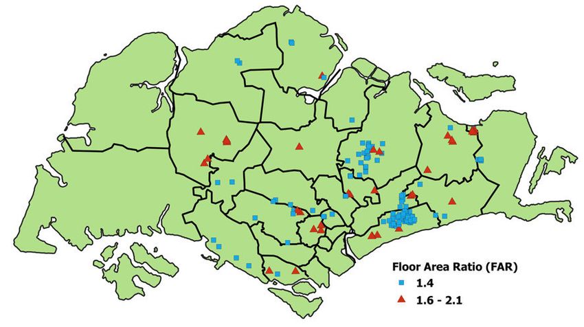
Our sample consists of 140 developments: 105 have a FAR of 1.4 and 35 have a FAR between
1.6 and 2.1. Figure 1 plots the developments on a map with postal district boundaries, a geo-
5graphic demarcation commonly used by developers and agents. The blue squares are 1.4 FAR
developments, and the red triangles are 1.6 to 2.1 FAR developments. We can see that both types
of developments are spread out across Singapore. In some robustness checks, we restrict the sam-
ple to developments in postal districts with both FAR categories so as to minimize differences in
unobserved neighborhood amenities.
We collected the following variables from planning documents from URA SPACE for each
development: (1) date of submission of the construction plan, (2) total number of housing units,
(3) floor area, and (4) realized floor area ratio. We compute lot size from the ratio of floor area
and the realized floor area ratio.
We define the density of a development as the total number of housing units in the development
per square meter of land. In Panel A of Table 1, we see that the average density of sample
developments was 0.023 housing units per square meter of land. Density was higher in the 1.6-2.1
FAR developments (0.026 units per meter of land) than 1.4 FAR developments (0.021 units per
meter of land).
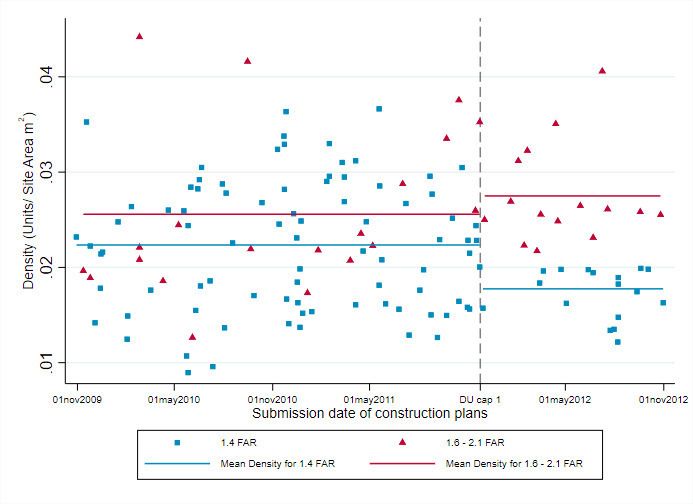
Figure 2 plots the densities of 1.4 FAR developments in blue squares and 1.6-2.1 FAR devel-
opments in red circles by the date of submission of construction plans. The effective date of the
policy change is represented by the dashed vertical line. The blue horizontal lines are the mean
densities of 1.4 FAR developments, before and after the policy change. The red horizontal lines
are the mean densities of 1.6-2.1 FAR developments, before and after the policy change.
We see that not only did the density of 1.4 FAR developments fall substantially after the policy
change but that the fall was more pronounced compared to the increase in density of 1.6-2.1 FAR
developments. In other words, the difference in the mean density of 1.4 FAR and 1.6-2.1 FAR
developments increased after the policy change, which supports our identification scheme that uses
the decrease in 1.4 FAR density after the policy change relative to the unregulated control group
of 1.6-2.1 FAR developments.
Further support for the identification scheme is given in Table 2, which computes how the
difference in average density by FAR changed after the policy date. In Panel A, we see in the last
row of column 1 that the 1.4 FAR developments were 0.135 log points less dense (12.6%) than 1.6
to 2.1 FAR developments. After the policy change, in column 2, the difference increases to 0.438
6log points, or 35.5%. In the last row of column 3, the difference in these differences is 0.304 log
points, or a 26.2% difference in density, which is significant at 1%.
In Panel B, we make a similar calculation but use a placebo policy change dated one year earlier
than the actual policy date. The before period is from the beginning of the sample, January 1,
2010, to the placebo policy date of November 24, 2010. The after period is from that date until the
actual policy date, November 24, 2011. In the last row, the differences in density are smaller using
the placebo policy date, including the difference-in-differences estimate of -0.129 log points in the
last row of column 6 (12.1% difference), which is not significant at any conventional significance
level. This evidence suggests that the reduction in density among 1.4 FAR developments after the
policy change is driven by the policy change itself.
We collected facilities information such as the presence of a swimming pool, barbecue area,
gym, tennis court, sauna, jacuzzi, etc. from condo websites and real estate websites such as prop-
ertyguru.com.sg. We collected Construction Quality Assessment System (CONQUAS) data from
the Building and Construction Authority, which includes a quality assessment of the structural,
architectural, and mechanical engineering works of developments. We computed distance to the
nearest Mass Rapid Transit (MRT) station, Singapore’s public rail system, and the distance to
the Central Business District from geocoordinates extracted from OneMap. Finally, we note that,
as a former British colony, Singapore follows the British leasehold system in which land is either
freehold, i.e., owned in perpetuity, or leased from a freeholder, usually the government, for a certain
number of years. About 23.6% of the developments are on land with 99-year leases. The remaining
leases are either 999 years or freehold. For further details on the leasehold system in Singapore,
readers may refer to Fesselmeyer et al. (2021).
Summary statistics of these development-level variables for the sample and broken down by
FAR can be found in Panel A of Table 1.
3.2 Transaction data
Transaction data is available from the REALIS database, which contains records of caveats of
private residential properties. The data includes housing-unit level information such as the date
of sale, transaction price, floor area, age, and floor. We collected new transactions (transactions
7between the developer and the first buyer) for the 140 developments included in the analysis. The
20,713 transactions span from 2010 to 2017. Because it takes several years to sell all units in
a development, we observe transactions of both effected and uneffected developments for several
years after the submission of construction plans.
Pabel B of Table 1 contains the summary statistics of housing unit-level variables, including a
breakdown by FAR. The main outcome variable of interest is transaction price per square meter
(deflated to 2000 SGD values). The average is SGD 9,626.65, or about USD 6,876. On average,
condominiums in 1.4 FAR developments sold for a higher price than those in 1.6-2.1 FAR develop-
ments, SGD 9,777.40 per square meter vs. SGD 9,475.49 per square meter (USD 6,983 vs. USD
6,768). The average deflated transaction price was SGD 804,677.80 (USD 574,770), with 1.4 FAR
condominiums selling for SGD 772,926.70 and 1.6-2.1 FAR condominiums sold for SGD 836,511.80
(USD 552,091 and USD 597,508). The differences in density and unit size could at least partially
explain the difference in prices. Units in 1.6-2.1 FAR developments tend to be larger. They aver-
aged around 90 square meters in size compared to 82 square meters for the 1.4 FAR condominiums.
We also note that the 1.4 FAR buildings are shorter than 1.6-2.1 FAR buildings, as expected. The
average floor of 1.4 FAR condominiums is 3.3 while the average floor of 1.6-2.1 FAR condominiums
is 8.4.
4 Empirical Strategy
One goal of this paper is to estimate the impact of density on residential prices. The main identi-
fication problem is that density is likely endogenous because any unobservable, e.g., neighborhood
quality, that affects price is also likely to affect how many units the developer decides to build. In
order to estimate the causal effect of density on price we use the policy restriction on the number
of housing units in 1.4 FAR developments to construct an instrumental variable, measuring how
density changed after the policy for 1.4 FAR developments compared to the control group of 1.6-2.1
FAR developments that were unaffected by the policy change, while including a large set of unit-
and development-level characteristics and geographic and temporal fixed effects.
8Specifically, the main equation of interest is:
ln Pijt = 0 + 1 F AR14j + 2 P OSTt + ln Dj + Xij + ⌧jt + ✏ijt , (2)
where Pijt is the (deflated) price per square meter of condominium i in development j in period
t, F AR14j is a 1.4 FAR development dummy variable, P OSTt is a post-policy change dummy
variable, Dj is the density of the development (the number of housing units in the development
divided by the lot size in meters), Xij are observed characteristics, ⌧jt are time and location fixed
effects, and ✏ijt is an idiosyncratic error. The parameter of interest is , the price elasticity with
respect to density.
The first stage is given by
ln Dj = ↵0 + ↵1 F AR14j + ↵2 P OSTt + ↵3 F AR14j × P OSTt + µXij + ⌧jt + ⌫ijt , (3)
where ⌫ijt is an idiosyncratic error. The interaction term F AR14j × P OSTt is our instrument for
density, allowing us to infer the exogenous variation in ln Dj . Given what we know of the Singapore
housing market, including what we saw in Figure 2 and Table 2, and the intention of the regulation,
the expectation is that ↵1 < 0 and ↵3 < 0, that is, 1.4 FAR developments were less dense than 1.6
to 2.1 FAR developments before the policy change and that the difference in densities between the
two FAR categories grew larger after the policy change.
5 Results
5.1 Primary regression results and robustness checks
Table 3 reports our primary results. Columns 1 and 2 include the estimated effect of log density
on log price per square meter, including housing-unit characteristics (floor fixed effects and a
quadratic of area in meters), sales year fixed effects, and postal district fixed effects. Columns 3
and 4 add development-level characteristics (a 99-year leasehold dummy, a special-neighborhood
dummy, the log distance to the CBD and to the nearest MRT station, the number of facilities in
the development, and whether the development was CONQUAS assessed and an interaction with
9CONQUAS quality score). Columns 5 and 6 add a more flexible time trend, with sales year fixed
effects for each postal district. The reason for adding these additional explanatory variables is to
control for the potential correlation between housing quality and development density. The odd
columns 1, 3, and 5 contain OLS estimates. The even columns 2, 4, and 6 contain two-stage least
squares estimates. The third-to-last row of the table reports the F -statistic of the instrument in
the first stage, a check on whether the instrument has “enough” explanatory power.
The specification in column 4 with housing-unit and dwelling-unit characteristics and a common
time trend of sales year fixed effects, estimated using two-stage least squares, is our preferred
approach. We use it and some variants in several robustness checks and related regressions below.
There is a clear pattern across the different results in Table 3: increased density caused price to
be lower. The coefficient estimate on log density is negative and significant for all two-stage least
squares estimates and for 2 out of the 3 OLS estimates. Consider column 2, with an estimate of
-0.815 on log density, which is significant at the 1% level, indicating that a 1% increase in density
leads to 0.56% decrease in price per square meter. The results reported in columns 4 and 6 show
that controlling for various observed housing characteristics indeed reduces the estimated negative
impact of density on housing price, which is consistent with the hypothesis that developers tend
to build higher quality houses in low density developments. In the specification with the most
controls, column 6, the density elasticity is -0.481. We also note that the F -statistic on the
instrument is around 17 or higher, indicating that the instrument is not weak according to the
10 rule-of-thumb (Stock and Yogo, 2003), and that the two-stage least square estimate on log
density is more negative than the corresponding OLS estimate for each specification pair, which is
consistent with the expectation that OLS is upward biased due to unobserved quality.
In Table 4, we re-estimate the regressions from Table 3 but restrict the sample to transactions
of developments in postal districts that contained at least one 1.4 FAR development and one 1.6-2.1
FAR development. This robustness check is meant to ensure that each treated development has
at least one corresponding control development nearby to minimize the influence of unobserved
neighborhood amenities. The results are similar: density has a negative effect on price. Further,
the two-stage least square estimates in columns 2, 4, and 6 are very similar in magnitude and
significance to those in Table 3.
10In Table 5, we examine whether the impact of density on price depends on the size of the
housing unit purchased. In column 1, we re-estimate the main specification on a sample consisting
of only shoebox units. We see that an increase in density of 1% decreases price per square meter by
0.6%. In column 2, we estimate the model using a subsample of units larger than 50 square meters
(that is, we exclude shoebox units). The estimate is similar to the Table 3, column 4 estimate,
indicating a decrease in price per square meter of about 0.3%. The larger effect estimated in the
shoebox subsample might reflect the premium shoebox dwellers with a small amount of private
space put on having fewer neighbors with whom to share the common areas of the development.
5.2 Changes in development composition
In this subsection, we consider how developers adjusted their designs, beyond density, in order to
meet the new regulation. Specifically we consider whether developers changed the composition of
the developments they built after the policy change by examining the distribution of shoebox units
(50 square meters or less), medium-sized units (more than 50 square meters to 106 square meters,
the 75th percentile), and large units (106 square meters and larger) across FAR category and time.
We then measure how composition changes affected price.
Figures 3 to 5 contain histograms of the composition of developments by FAR and period. Panel
(a) of Figure 3 contains the share of shoebox units in 1.4 FAR developments before the policy. There
was a wide range of outcomes. The proportion of shoebox units in some developments was very
small but there were many developments in which over 50% of the housing units, some even higher
than 90%, which were shoeboxes. We can contrast this with the distribution of shoeboxes in 1.6-2.1
FAR developments before the policy: a large majority of developments had very small proportions
of shoebox units.
Panel (b) contains the proportion of shoebox units in 1.4 FAR developments after the policy
change. We see, compared to panel (a), that there was a significant decrease in the share of
developments with a substantial proportion of shoebox units. Panels (a) and (b) clearly show that
developers responded to the policy by building fewer very small units. Panel (d) shows that the
developers of 1.6-2.1 FAR developments did not change their layouts substantially.
Figure 4 contain similar histograms of medium-sized units. Compared to the shoebox his-
11tograms, there is a less substantial difference between 1.4 FAR developments and 1.6-2.1 FAR
developments before the policy change. Panels (a) and (b) show that there was a decrease in the
share of 1.4 FAR developments with a small proportion of medium-sized units after the policy
change.
Figure 5 contains histograms of large units. These histograms show the least heterogeneity.
The 1.4 FAR developments and the 1.6-2.1 FAR developments show a similar distribution before
and after the policy change. Both development types exhibit an increase in the proportion of large
units after the policy change.
Overall, we can conclude from the histograms that developers of 1.4 FAR lots were building
developments with a very high proportion of shoeboxes before the introduction of the policy. In
order to adhere to the regulatory requirement, developers decreased the proportion of shoebox
units, while also increasing the proportion of medium-sized and large units, thereby increasing the
average unit size of a development.
In Table 6, we consider how unit composition within developments affected price. In column 1
our explanatory variable of interest is the percentage of shoebox units in the development, column
2 the percentage of medium-sized units in the development, and column 3 the percentage of large
units in the development. We continue to use the interaction between the 1.4 FAR dummy and
the post-policy change dummy as an instrument.
The results are intuitively appealing, given our findings in the density regressions and the
histograms of size distributions. In column 1, we see that a 1 percentage-point increase in shoebox
units decreased price per square meter by 0.3%, and the result is statistically significant. In column
2, the proportion of medium-sized units had no significant effect on price (and that the instrument
does not provide a strong response, with an F -statistic of 2.76). In column 3, we see that a greater
proportion of large units increased price: a 1 percentage-point increase caused price per square
meter to increase by 0.2%.
126 Profit analysis
The policy reduced the number of units a developer can build on a 1.4 FAR lot by increasing
the required average unit size, which we have seen was achieved by reducing the proportion of
small units and increasing the proportion of medium-sized and large units. The proportion of
shoebox units in 1.4 FAR developments declined by 14.7 percentage points from 32.4% in the pre-
policy period to 17.7% in the post-policy period, and the proportion of medium-sized and large
units increased by 8.2 and 6.2 percentage points, respectively. Because price per square meter
is decreasing in unit size, that is, price per square meter is higher for smaller units than larger
units, the change in size composition away from small units could have reduced the mean price per
square meter of the development, which could explain why developers only reduced density after
the regulation was introduced. Alternatively, a reduction in density could have instead benefited
developers because, all else equal, it raises the price for units of all sizes because households dislike
density. If the developers or their sales staff did not fully internalize this externality because they
were not aware of its extent or were not incentivized to do so it is possible that the regulation
actually made developers better off.
To examine this possibility more closely, we predict the price of a 1.4 FAR development with
the average size composition before and after the policy change, finding that the price per square
meter for the entire development was higher after the implementation of the regulation. Moreover,
built-up area did not change. The average realized gross plot ratio of 1.4 FAR developments
was constant at 1.51 (which includes bonus allowances that developers took advantage of, before
and after the policy). Since built-up area did not change, cost differences were minimal, and the
predicted increase in price per square meter indicates that profit per square meter increased. This
suggests that developers built too many shoebox units in the pre-policy period, foregoing some
profit.
We present the calculations in Tables 7 and 8. In Table 7, we categorize units into 3 sizes,
shoebox, medium-sized, and large units. In Table 8, we use a finer categorization of unit sizes,
creating 10 bins based on floor area percentiles of the transaction data.
Column 1 contains the mean area in square meters of each category. Columns 2 and 3 contain
13the average proportion of each size category, before and after the regulation, and columns 4 and 5
contain the mean log density of 1.4 FAR developments, before and after the regulation. Columns 6
and 7 contain the predicted log price per square meter using the 2SLS regression estimates in Table
3, column 4 (panel A) and in Table 3, column 6 (panel B) for units with column 1 area and log
density reported in columns 4 and 5, respectively. We used median values for other covariates. In
columns 8 and 9, we transform the predicted log price in columns 6 and 7 to price per square meter
dp), where
using the formula p̂ = exp(ˆ 2 /2) exp(ln 2 is the variance of the error term. Average
price in the last row of columns 8 and 9 in each panel is the weighted average price per square
meter using price in columns 8 and 9 and the shares in columns 2 and 3.
In both panels of Table 7, we see that price per per square meter is higher after the policy
regulation than before. In Panel A, price per per square meter is SGD 7,671.47 vs. SGD 7,587.13,
a 1.1% difference, and in Panel B, it is SGD 7,450.64 vs. SGD 7,223.70, a 3.1% difference. The
small differences are not surprising otherwise one might expect the developer to be more aware of
the externality and/or more active in minimizing its effect.
In Table 8, we see again that the average developer did better under the regulation. Price is
1.1% higher, SGD 7,690.35 in the post-policy change period vs. SGD 7,609.79 in the pre-policy
period.
7 Conclusion
In this paper, we use the introduction of a regulation governing the average unit size of low-
density residential developments in Singapore to measure the causal impact of very local density on
housing prices. We find that price per square meter is lower when density is greater, confirming that
households dislike within-development density. We also find that developers reduced the proportion
of small shoebox units after the policy change both absolutely and in comparison to a control group
of developments unaffected by the regulation. Finally, we show that developers of restricted lots
received a higher overall price per square meter after the introduction of the regulation, and since
built up area and construction costs did not change, this indicates that profits also increased. We
speculate that this unexpected outcome may have occurred because developers did not understand
14the extent of the density externality, which also suggests that policymakers might not either.
The regulation we use to identify the effect of density occurred in pre-pandemic times. A
potential extension of our research is to measure whether people’s dislike for density has increased
since 2020 as lockdowns and social distancing has become part of our lives. We leave this question
for future work.
15References
Ahlfeldt, G. M. and Pietrostefani, E. (2019). The economic effects of density: A synthesis.
Journal of Urban Economics, 111(April):93–107.
Ahlfeldt, G. M., Redding, S., Sturm, D., and Wolf, N. (2015). The economics of density:
Evidence from the Berlin Wall. Econometrica, 83:2127–2189.
Arango, T. (2021). ‘We Are Forced to Live in These Conditions’: In Los Angeles, Virus Ravages
Overcrowded Homes. New York Times, retrieved on July 14, 2021 from
https://www.nytimes.com/2021/01/23/us/los-angeles-crowded-covid.html.
Brueckner, J. and Largey, A. (2008). Social interaction and urban sprawl. Journal of Urban
Economics, 64:18–34.
Chan, Y.-K. (1999). Density, Crowding, and Factors Intervening in Their Relationship: Evidence
from a Hyper-Dense Metropolis. Social Indicators Research, 48(1):103–124.
Ciccone, A. and Hall, R. (1996). Productivity and the density of economic activity. American
Economic Review, 86(1):54–70.
Department of Statistics Singapore (2020). Data on Households.
Fang, W. and Wahba, S. (2020). Urban density is not an enemy in the coronavirus fight:
Evidence from China. World Bank Blogs.
Fesselmeyer, E., Liu, H., and Salvo, A. (2021). Declining discount rates in Singapore’s market
privately developed apartments. Journal of Applied Econometrics, forthcoming.
Fesselmeyer, E., Seah, K. Y. S., and Kwok, J. C. Y. (2018). The effect of localized density on
housing prices in Singapore. Regional Science and Urban Economics, 68:304–315.
Glaeser, E. and Gyourko, J. (2018). The economic implications of housing supply. Journal of
Economic Perspectives, 32(1):3–29.
Gómez-Jacinto, L. and Hombrados-Mendieta, I. (2002). Multiple effects of community and
household crowding. Journal of Environmental Psychology, 22(3):233–246.
16Gray, A. (2001). Definitions of crowding and the effects of crowding on health: A literature
review. New Zealand Ministry of Social Policy.
Gyourko, J. and Molloy, R. (2015). Regulation and Housing Supply. In Handbook of Regional and
Urban Economics, volume 5, pages 1289–1337. Elsevier.
Hilber, C. A. and Vermeulen, W. (2016). The Impact of supply constraints on house prices in
England. Economic Journal, 126(591):358–405.
Ihlanfeldt, K. R. (2007). The effect of land use regulation on housing and land prices. Journal of
Urban Economics, 61(3):420–435.
Kiefer, P. (2020). Will we ever trust crowds again? National Geographic, retrieved on July 14,
2021 from https://www.nationalgeographic.com/science/article/coronavirus-will-we-ever-trust-
crowds-again-cvd.
Lee, J. (2016). Measuring the value of apartment density?: The effect of residential density on
housing prices in Seoul. International Journal of Housing Markets and Analysis, 9(4):483–501.
Lerner, M. (2020). Choosing the suburbs over city life during the pandemic. Washington Post,
retrieved on July 14, 2021 from
https://www.washingtonpost.com/realestate/choosing-the-suburbs-over-city-life-during-the-
pandemic/2020/10/15/01c94c5e-e716-11ea-97e0-94d2e46e759b story.html.
Molloy, R. (2020). The effect of housing supply regulation on housing affordability: A review.
Regional Science and Urban Economics, 80(July 2017):103350.
Stock, J. H. and Yogo, M. (2003). Testing for weak instruments in linear IV regression.
Identification and Inference for Econometric Models: Essays in Honor of Thomas Rothenberg,
2001(August 2001):80–108.
Tan, Y., Wang, Z., and Zhang, Q. (2020). Land-use regulation and the intensive margin of
housing supply. Journal of Urban Economics, 115(July 2017):103199.
Tang, B. and Yiu, C. (2010). Space and scale: A study of development intensity and housing
price in Hong Kong. Landscape and Urban Planning, 96(3):172–182.
17Urban Redevelopment Authority (2011). Circular Number URA/PB/2011/14-DCG. Technical
report, URA.
Urban Redevelopment Authority (2012). Circular Number URA/PB/2012/14-DCG. Technical
report, URA.
Zabel, J. and Dalton, M. (2011). The impact of minimum lot size regulations on house prices in
Eastern Massachusetts. Regional Science and Urban Economics, 41(6):571–583.
Zhong, Y. and Teirlinck, B. (2020). Density and its effect on COVID-19 spread. retrieved on July
14, 2021 from https://edc.nyc/insights/density-and-its-effect-on-covid-19-spread.
18Table 1: Summary statistics
Panel I: Development-level summary statistics
All developments 1.4 FAR 1.6 - 2.1 FAR
Mean Std Dev Mean Std Dev Mean Std Dev
Density (housing units per m2 ) 0.023 0.007 0.021 0.006 0.026 0.007
Housing units 160.1 202.5 106.9 151.8 319.7 249.3
99-year leasehold 0.236 0.426 0.162 0.370 0.457 0.511
Special neighborhood 0.421 0.496 0.552 0.500 0.029 0.169
Gym 0.686 0.466 0.629 0.486 0.857 0.355
Swimming pool 0.971 0.167 0.962 0.192 1.000 0.000
Tennis court 0.214 0.412 0.124 0.331 0.486 0.507
Jacuzzi 0.336 0.474 0.333 0.474 0.343 0.482
Sauna 0.186 0.390 0.152 0.361 0.286 0.458
Barbecue 0.807 0.396 0.790 0.409 0.857 0.355
Total number of facilities 3.200 1.405 2.990 1.411 3.829 1.200
CONQUAS-assessed 0.393 0.490 0.267 0.444 0.771 0.426
CONQUAS score 90.06 6.30 87.96 7.41 92.32 3.83
Distance to the CBD (m.) 6,816.3 3,561.6 6,527.3 3,098.3 7,683.6 46,32.9
Distance to MRT station (m.) 809.1 406.2 812.9 383.7 797.6 473.3
Proportion of shoebox units 0.309 0.294 0.344 0.301 0.205 0.248
Proportion of medium-sized units 0.500 0.229 0.478 0.227 0.568 0.226
Proportion of large units 0.187 0.198 0.174 0.195 0.226 0.203
Developments 140 105 35
Panel II: Housing unit-level summary statistics
All developments 1.4 FAR 1.6 - 2.1 FAR
Mean Std Dev Mean Std Dev Mean Std Dev
Transaction price (2000 SGD) 804,677.80 451,094.30 772,926.70 470,915.80 836,511.80 427,969.60
Price per m2 (2000 SGD) 9,626.65 2,769.77 9,777.40 2,701.62 9,475.49 2,828.52
Floor 5.86 4.54 3.30 1.58 8.42 5.06
Area (m2 ) 85.91 39.07 81.76 42.76 90.08 34.48
Sale year 2012 1.14 2012 1.03 2012 1.23
Observations 20,713 10,370 10,343
19Table 2: Mean log density by FAR before and after the policy change and a placebo test
Panel A. Actual policy Panel B. Placebo test
Before After (2)-(1) Before After (5)-(4)
(1) (2) (3) (4) (5) (6)
1.4 FAR -3.850 -4.047 -0.197 -3.847 -3.852 -0.006
(0.036) (0.008) (0.053) (.061) (0.009) (0.074)
1.6 to 2.1 FAR -3.715 -3.608 0.107 -3.777 -3.653 0.124
(0.004) (0.008) (0.084) (0.010) (0.009) (0.143)
Difference -0.135 -0.438 -0.304 -0.070 -0.199 -0.129
(0.078) (0.059) (0.098) (0.130) (.089) (0.157)
Note: Each cell contains mean log density, with the standard error in parentheses below. In panel A,
the before period includes all developments with plans submitted before the policy date, November
24, 2011. The after period includes all developments with plans submitted after the policy date. In
panel B, the placebo test imposes a placebo policy date of November 24, 2010. The before period
includes all developments with plans submitted before the placebo policy date. The after period
includes all developments with plans submitted after the placebo policy date, up to the actual policy
date.
20Table 3: The effect of log density on log price per square meter
(1) (2) (3) (4) (5) (6)
OLS 2SLS OLS 2SLS OLS 2SLS
Log density -0.066* -0.815*** -0.070*** -0.305** -0.033 -0.481***
(0.035) (0.273) (0.026) (0.132) (0.027) (0.175)
Constant 9.597*** 7.093*** 11.310*** 10.247*** 11.246*** 9.133***
(0.123) (0.908) (0.345) (0.705) (0.368) (0.948)
Unit characteristics Yes Yes Yes Yes Yes Yes
Development characteristics No No Yes Yes Yes Yes
Postal district fixed effects Yes Yes Yes Yes Yes Yes
Sales year fixed effects Yes Yes Yes Yes Yes Yes
Postal district × sales year f.e. No No No No Yes Yes
Weak IV F-statistic 16.98 30.2 21.37
R-squared 0.831 0.862 0.880
Observations 20,713 20,713 20,713 20,713 20,713 20,713
Notes: *** pTable 4: The effect of log density on log price per square meter, geographically restricted sample
(1) (2) (3) (4) (5) (6)
OLS 2SLS OLS 2SLS OLS 2SLS
Log density -0.008 -0.739*** -0.002 -0.370*** 0.003 -0.506***
(0.030) (0.205) (0.029) (0.120) (0.032) (0.175)
Constant 9.783*** 7.357*** 11.599*** 10.286*** 11.388*** 9.507***
(0.109) (0.676) (0.379) (0.567) (0.407) (0.757)
Unit characteristics Yes Yes Yes Yes Yes Yes
Development characteristics No No Yes Yes Yes Yes
Postal district fixed effects Yes Yes Yes Yes Yes Yes
Sales year fixed effects Yes Yes Yes Yes Yes Yes
Postal district × sales year f.e. No No No No Yes Yes
Weak IV F-statistic 28.17 37.66 21.94
R-squared 0.811 0.569 0.847 0.802 0.859 0.795
Observations 16,215 16,215 16,215 16,215 16,215 16,215
Notes: *** pTable 5: Shoebox and non-shoebox sub-samples
(1) (2)
Shoebox Non-shoebox
Log density -0.818** -0.304**
(0.386) (0.151)
Constant 12.173*** 10.419***
(0.800) (0.770)
Unit characteristics Yes Yes
Development characteristics Yes Yes
Postal district fixed effects Yes Yes
Sales year fixed effects Yes Yes
Weak IV F-statistic 5.32 28.61
Observations 4,066 16,647
Notes: *** pTable 6: The effect of development composition on log price per square meter
(1) (2) (3)
2SLS 2SLS 2SLS
Percentage of shoebox units -0.003**
(0.002)
Percentage of medium-sized units -0.006
(0.004)
Percentage of large units 0.002**
(0.001)
Constant 11.410*** 11.704*** 11.442***
(0.424) (0.445) (0.359)
Unit characteristics Yes Yes Yes
Development characteristics Yes Yes Yes
Postal district fixed effects Yes Yes Yes
Sales year fixed effects Yes Yes Yes
Weak IV F-statistic 20.17 2.76 57.27
Observations 20,713 20,713 20,713
Notes: *** pTable 7: Average price per m2 before and after the policy change for the average 1.4 FAR development
Proportion of Log price Price
Area (m2 ) total units Log density per m2 per m2
(1) (2) (3) (4) (5) (6) (7) (8) (9)
Before After Before After Before After Before After
A. Table 3, col. 4
Shoebox 42.24 0.313 0.170 -3.958 -4.081 9.037 9.075 8,454.97 8,778.16
Medium-sized 77.12 0.486 0.572 -3.958 -4.081 8.923 8.961 7,544.59 7,832.99
Large 145.28 0.202 0.258 -3.958 -4.081 8.750 8.787 6,342.47 6,584.92
Ave. price 7,587.13 7,671.47
B. Table 3, col. 6
Shoebox 42.24 0.313 0.170 -3.958 -4.081 8.995 9.054 8,105.35 8,599.57
Medium-sized 77.12 0.486 0.572 -3.958 -4.081 8.873 8.933 7,180.25 7,618.06
Large 145.28 0.202 0.258 -3.958 -4.081 8.687 8.746 5,959.81 6,323.21
Ave. price 7,223.70 7,450.64
Shoebox units are units with 50 square meters or less of floor area, medium-sized units have more than 50 square meters
up to 106 square meters (the 75th percentile), and large units have more that 106 square meters. Column (1) contains
the mean area in square meters of shoebox, medium-sized, and large units of 1.4 FAR developments. Columns (2) and (3)
contain the development proportion of the three unit types, before and after the regulation. Columns (4) and (5) contain
the mean log density of 1.4 FAR developments, before and after the regulation. Columns (6) and (7) contain the predicted
log price per square meter using the 2SLS regression estimates in Table 3, column (4) (panel A) and in Table 3, column (6)
(panel B) for units with column (1) area, in postal district 17, on the 3rd floor, and sold in 2012, and log density reported
in columns (4) and (5), respectively. In columns (8) and (9), we transform the predicted log price in columns (6) and (7)
dp), where σ 2 is the variance of the error term. Average
to price per square meter using the formula p̂ = exp(σ̂ 2 /2) exp(ln
price in the last row of columns (8) and (9) in each panel is the weighted average price per square meter using price in
columns (8) and (9) and the shares in columns (2) and (3).
25Table 8: Average price per m2 before and after the policy change for the average 1.4 FAR development
Proportion of Log price Price
Size (m2 ) total units Log density per m2 per m2
(1) (2) (3) (4) (5) (6) (7) (8) (9)
Before After Before After Before After Before After
Decile 1 37.85 0.150 0.034 -3.958 -4.081 9.053 9.09 8,587.33 8,915.59
Decile 2 43.43 0.078 0.115 -3.958 -4.081 9.033 9.07 8,419.89 8,741.74
Decile 3 49.20 0.106 0.034 -3.958 -4.081 9.013 9.051 8,253.80 8,569.30
Decile 4 56.95 0.104 0.102 -3.958 -4.081 8.987 9.025 8,041.80 8,349.20
Decile 5 69.56 0.087 0.164 -3.958 -4.081 8.946 8.984 7,722.06 8,017.24
Decile 6 77.86 0.094 0.090 -3.958 -4.081 8.921 8.959 7,527.92 7,815.67
Decile 7 89.35 0.102 0.090 -3.958 -4.081 8.887 8.925 7,278.49 7,556.72
Decile 8 103.24 0.098 0.145 -3.958 -4.081 8.849 8.887 7,005.27 7,273.05
Decile 9 121.46 0.086 0.108 -3.958 -4.081 8.803 8.84 6,689.55 6,945.26
Decile 10 175.55 0.095 0.117 -3.958 -4.081 8.693 8.731 5,995.29 6,224.46
Ave. price 7,609.79 7,690.35
Deciles of floor area are computed using transactions in 1.4 FAR developments. Column (1) contains the mean area
in square meters by unit area decile. Columns (2) and (3) contain the development proportion of the three unit
types, before and after the regulation. Columns (4) and (5) contain the mean log density of 1.4 FAR developments,
before and after the regulation. Columns (6) and (7) contain the predicted log price per square meter using the 2SLS
regression estimates in Table 3, column (4) (panel A) and in Table 3, column (6) (panel B) for units with column
(1) area, in postal district 17, on the 3rd floor, and sold in 2012, and log density reported in columns (4) and (5),
respectively. In columns (8) and (9), we transform the predicted log price in columns (6) and (7) to price per square
dp), where σ 2 is the variance of the error term. Average price in the
meter using the formula p̂ = exp(σ̂ 2 /2) exp(ln
last row of columns (8) and (9) in each panel is the weighted average price per square meter using price in columns
(8) and (9) and the shares in columns (2) and (3).
26Figure 1: FAR 1.4 and FAR 1.6 to 2.1 developments with postal district boundaries
27Figure 2: Development density over time by Floor Area Ratio (FAR)
28Figure 3: Distribution of shoebox units by FAR, before and after policy change
(a) 1.4 FAR developments, before policy change (b) 1.4 FAR developments, after policy change
(c) 1.6 - 2.1 FAR developments, before policy change (d) 1.6 - 2.1 FAR developments, after policy change
29Figure 4: Distribution of medium-sized units by FAR, before and after policy change
(a) 1.4 FAR developments, before policy change (b) 1.4 FAR developments, after policy change
(c) 1.6 - 2.1 FAR developments, before policy change (d) 1.6 - 2.1 FAR developments, after policy change
30Figure 5: Distribution of large units by FAR, before and after policy change
(a) 1.4 FAR developments, before policy change (b) 1.4 FAR developments, after policy change
(c) 1.6 - 2.1 FAR developments, before policy change (d) 1.6 - 2.1 FAR developments, after policy change
31You can also read