HYPERSPECTRAL BAND SELECTION BASED ON IMPROVED AFFINITY PROPAGATION
←
→
Page content transcription
If your browser does not render page correctly, please read the page content below
HYPERSPECTRAL BAND SELECTION BASED ON IMPROVED AFFINITY PROPAGATION

              Qingyu Zhu1, Yulei Wang1,2, Fengchao Wang1, Meiping Song1, Chein-I Chang1,3

  1
    Center for Hyperspectral Imaging in Remote Sensing (CHIRS), Information and Technology College,
                           Dalian Maritime University, Dalian 116026, China;
  2
    State Key Laboratory of Integrated Services Networks, School of Telecommunications Engineering,
                                 Xidian University, Xian 710071, China
    3
      Department of Computer Science and Electrical Engineering, University of Maryland, Baltimore
                                  County, Baltimore, MD 21250, USA

                       ABSTRACT                                low-dimensional space. The new feature is a combination of
                                                               original features. For example, principal component
Dimensionality reduction is a common method to reduce          analysis [2], local preservation projection [3], the other is
the computational complexity of hyperspectral images and       based on non-transformed feature selection, also known as
improve the classification performance. Band selection is      band selection. Compared with feature extraction, band
one of the most commonly used methods for dimensionality       selection can retain the physical information of the original
reduction. Affinity propagation (AP) is a clustering           data. It is an effective method to reduce the dimension.
algorithm that has better performance than traditional               AP is a sample-based clustering method. As a new
clustering methods. This paper proposes an improved AP         clustering algorithm, it was proposed by Frey and Dueck in
algorithm (IAP), which divides each intrinsic cluster into     2007 [4]. It does not need to specify the number of clusters
several subsets, and combines the information entropy to       in advance, and performs clustering based on the similarity
change the initial availability matrix to obtain a suitable    between sample points. Regarding all sample points as the
number of clustering results with arbitrary shapes. The        initial clustering exemplar, the AP executes fast and has
experimental results on the public hyperspectral data set      small errors, and the most representative features can be
show that the band combination selected by IAP has a better    found in a short time. It has been successfully applied to
classification accuracy compared with all bands data set and   face recognition [5] and wireless remote [6]. [7] combine
band subset by traditional AP algorithm.                       AP with ternary mutual information to measure the band
                                                               correlation of classification. In [8], the relationship between
                                                               hyperspectral data points is measured by two constraints,
  Index Terms — Hyperspectral images, affinity
                                                               and a good classification effect is achieved. AP controls the
propagation, improved affinity propagation , classification
                                                               number of identified clusters by parameters called
                                                               preferences, but only adjusting preferences cannot find all
                1. INTRODUCTION                                ideal cluster exemplars.
                                                                     This paper proposes an improved AP algorithm that
Hyperspectral images contain higher spatial resolution and
                                                               divides each intrinsic cluster into several subsets. In theory,
spectral resolution, providing rich information for the
                                                               this segmentation can be randomly, which can obtain
classification and identification of ground features [1].
                                                               suitable number of clustering results. IAP can find the same
However, when the training samples are limited, the
                                                               number or more ideal band subsets as AP.
classification accuracy will decrease as the band increases,
which is the "Hughes" phenomenon. In addition, the
correlation between adjacent bands is relatively high,                     2. ALGORITHM PROPOSED
causing information redundancy and increasing the amount
                                                               2.1. Affinity propagation
of calculation. Therefore, dimensionality reduction is
necessary.                                                     AP is a sample-based clustering method [4]. It selects real
     At present, the dimensionality reduction of               data points as exemplars, treats all sample points as initial
hyperspectral remote sensing images is mainly divided into     exemplars, and exchanges information between data points
two methods: one is feature extraction based on                until a representative sample set appears. AP takes the
transformation. The original data is spatially transformed     similarity between data points as input. The similarity is
through mathematical mapping and transformed to a              defined by the negative Euclidean distance. These
similarities can be symmetrical or asymmetrical. Similarity availability matrix, t is the number of iterations, is the
measure can be calculated as damping factor with range of [0.5, 1].
s ( xi , x j ) || xi x j ||2 2.2. Improved AP
(1)
The information entropy of an image can be used as a
s ( xi , x j ) represents the similarity of xi and x j in AP quantification standard for the image. The larger the
which is called preference. information entropy is, the more information the image
Two types of messages are passed in the AP contains. The information entropy I of a one-dimensional
algorithm, which are responsibility and availability. r ( xi , x j ) image can be expressed as
represents the numerical message sent from xi to candidate 255
exemplar x j , reflecting whether x j is suitable as the I p (i ) log p (i )
i 0 (5)
exemplar of point xi , a( xi , x j ) represents numeric message
sent from candidate exemplar x j to xi , reflecting Where p (i ) represents the probability that a pixel with a
grayscale value of i appears in the grayscale image.
whether xi chooses x j as its exemplar. The larger value of The initial availability matrix is an important factor
r ( xi , x j ) , the greater the probability that x j is the exemplar, leading to different exemplar sets. This paper proposes a
new method to change exemplar sets by changing the initial
and the greater probability that xi belongs to x j cluster. AP
availability matrix.
algorithm continuously updates the attractiveness and
attribution value of each point through an iterative process,
until a number of high-quality exemplars are generated, and Algorithm IAP
the remaining data points are assigned to the corresponding The preferences s ( xi , x j ) of band xi and band x j is
clusters. calculated according to formula (1).Thus, the similarity
Initially, the availabilities are set to zero, i.e.,
matrix S L L is formed, where L represents the total
a ( xi , x j ) 0 , updating with the following formula
number of bands of hyperspectral image.
r ( xi , x j ) s ( xi , x j ) max[ s ( xi , xk ) a ( xi , xk )] Input: S L L , number of sub-blocks: k .
k j
(2) Output: exemplar of each data point, i.e., selected band
subsets.
max[0, r ( xk , x j )] i j Steps:
k j 1.The information entropy of each band image is
a( xi , x j )
min[0, r ( x j , x j ) max[0, r ( xk , x j )] i j calculated according to formula (5), then arranged in
k j ,i
(3) descending order to ent , Permute S L L according
'
After each update, the exemplar x j of the current to ent and get the permuted S L L , that is:
sample xi can be determined, x j is the exemplar of the s ' ( xi , x j ) s (ent ( xi ), ent ( x j ))
(6)
maximum value of a ( xi , x j ) r ( xi , x j ) . If i j , then '
2.Divide matrix S L L into k blocks, that is:
sample x j is the exemplar of its own cluster, otherwise, xi
belongs to the cluster to which xk belongs. Finally, all the S '11 S '12 L S '1 k
exemplar points are found by the main diagonal elements of
S' S' L S '2 k
the decision matrix, which meet a ( xi , x j ) r ( xi , x j ) 0 . S ' 21 22 (7)
M M O M
In practical applications, search algorithms are prone
to shocks. Therefore, a damping coefficient is added to S 'k 1 S 'k 2 L S 'kk
ensure that the algorithm converges
k must be larger than 1 and less than L / 2 .
Rt 1 Rt 1 (1 ) Rt '
3. Use sub-matrix S11 '
, S 22 '
, S kk , as input of AP, then we
A t 1
A t 1
(1 ) A t
' ' '
(4) get k availability matrices A11 , A22 Akk .
' ' '
Where R and A represent the responsibility matrix and the 4. Combine A11 , A22 Akk as the input of the initial
availability matrix of AP to get the exemplar set I ' : is selected, and in order to ensure the fairness of
A11' experimental results, all algorithms use the same training
'
'
A22 and testing sets.
A (8)
O Table 1 shows Classification accuracy of all bands,
Akk' AP, IAP on Salinas scene,where the boldface indicates
The rest of matrix A' are all zeros. the optimal classification accuracy,For each method, the
5. Restore I : average OA, AA, Kappa, the number of selected bands
I ( xi ) ent ( I ' ( xi )) and the corresponding standard deviation in 30
(9)
6. Output exemplar of each data point, i.e., selected band independent runs are recorded. It can be seen that the
subsets. number of band combinations selected by AP and IAP is
fixed, and the experimental results won’t be changed
3. EXPERIMENTAL RESULTS
with the number of experiments, which also shows the
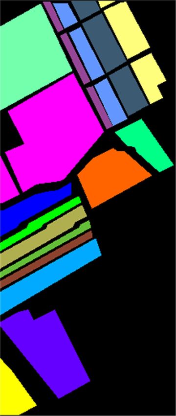
3.1. Dataset: Salinas scene stability of the algorithm. IAP obtains the highest
Salinas scene is a public hyperspectral data set acquired classification accuracies in terms of OA, AA, and kappa
by the AVIRIS sensor over Salinas Valley, California, indexes.
and with a spectral resolution of 3.7m per pixel and the
Table 1. Classification accuracy of all bands, AP, IAP on Salinas
spectral resolution is 10nm. The image size
scene
is 512 227 224 , including 20 water absorption bands,
Category All bands AP IAP
108-112, 154-167, and 224. After removing water
1 1 0.5 99.93 0.9 99.85 0.4
absorption bands, there are 204 bands remaining. Fig 1
2 99.87 0.4 99.74 0.7 99.71 0.6
shows the pseudo-color image of Salinas scene and 16
3 99.32 1.7 95.86 1.9 96.09 2.0
category distribution labels.
4 98.77 0.3 99.32 0.7 98.64 0.2
5 99.60 0.6 99.30 0.9 99.10 0.7
6 99.97 0.9 99.79 1.3 99.97 0.8
7 99.66 0.2 99.86 0.3 99.42 0.7
8 81.40 2.3 81.90 3.9 81.87 2.7
9 99.33 0.7 99.60 1.1 99.51 1.0
10 90.73 1.0 88.03 1.9 94.06 0.8
11 98.52 3.1 89.49 5.4 94.58 4.1
12 96.60 1.7 98.67 3.3 99.45 2.2
13 99.56 1.1 96.19 2.4 99.78 0.9
14 97.25 1.2 93.08 1.9 95.11 1.8
(a) (b)
15 74.23 1.1 70.17 1.7 72.62 0.9
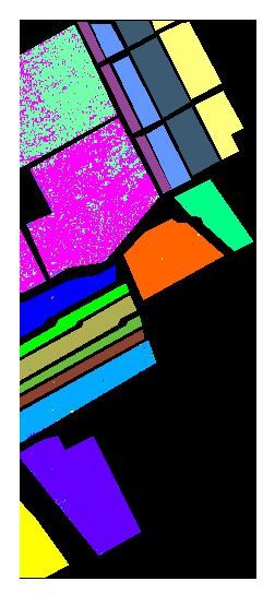
Fig 1. Salinas scene with 16 classes, with (a) pseudo-color of 16 97.93 1.2 98.52 2.3 98.52 1.7
Salinas scene and (b) Color ground-truth image with class labels
OA (%) 90.64 1.04 89.34 1.01 91.45 1.03
The experimental results are verified by
AA (%) 95.79 1.12 94.34 1.17 95.51 1.09
hyperspectral classification using support vector machine
Kappa (%) 88.15 0.74 88.48 1.80 90.45 0.95
(SVM) algorithm. Gaussian radial basis kernel function
No. band 204 0 7 0 8 0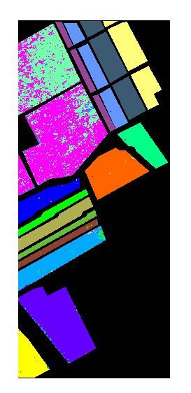
Fig 2 shows band subsets obtained by AP and IAP,                             5. ACKNOWLEDGEMENTS
where the white lines indicate the index of the selected band.
In order for a visual comparison of classification results,
Fig 3 shows classification maps of Salinas image using all                This work is supported by the National Nature Science
bands, band subsets by AP and IAP, respectively. It could be         Foundation of China (61801075), China Postdoctoral
shown from the results that, compared with AP, IAP has a             Science Foundation (No. 2020M670723), Open Research
better classification accuracy, which is even better than            Funds of State Key Laboratory of Integrated Services
using total bands.                                                   Networks, Xidian University (N0. ISN20-15) and the
                                                                     Fundamental Research Funds for the Central Universities
                                                                     (3132019341).

                                                                                        6. REFERENCES

                                                                     [1] M. Zhao, C.Y. Yu, M.P. Song and C.I. Chang, “A
                                                                         Semantic Feature Extraction Method for Hyperspectral
                                                                         Image Classification Based on Hashing Learning,”
                                                                         Workshop on Hyperspectral Image and Signal
                    (a)                (b)                               Processing:       Evolution      in   Remote    Sensing
                                                                         (WHISPERS), Amsterdam, Netherlands, 2018.
Fig 2. Results of AP and IAP, where white lines represent selected   [2] M.D. Farrell and R. M. Mersereau," On the Impact of
bands, with (a) AP and (b) IAP                                           PCA Dimension Reduction for Hyperspectral
                                                                         Detection of Difficult Targets," IEEE Geosci. Remote
                                                                         Sens. Lett., vol. 2, no. 2, pp.192-195, 2005.
                                                                     [3] L. Lei, S. Prasad, J. E. Fowler, and L. M. Bruce,
                                                                         “Locality-preserving Dimensionality Reduction and
                                                                         Classification for Hyperspectral Image Analysis,"
                                                                         IEEE Trans. Geosci. Remote Sens., vol. 50, no. 4, pp.
                                                                         1185-1198, 2012.
                                                                     [4] B.F. Frey and D. Dueck, “Clustering by Passing
                                                                         Messages Between Data Points," Science, vol. 315,
                                                                         pp.972- -976, 2007.
                                                                     [5] R. Rina, B.M. Achmad, J. Asep and S. Adang,
                                                                         “Clustering Grey-Scale Face-Images Using Modified
                                                                         Adaptive Affinity Propagation with a New Preference
                                                                         Model,” International Conference on Informatics and
                                                                         Computing (ICIC), Palembang, Indonesia, 2018.
         (a)                  (b)                     (c)            [6] S. Park, H.S. Jo, C. Mun and J.G. Yook, “Radio
                                                                         Remote Head Clustering with Affinity Propagation
Fig 3. Classification maps of the Salinas image, where (a)-(c) are
                                                                         Algorithm in C-RAN,” IEEE Conference on Vehicular
classification maps by all bands, AP, IAP, respectively.                 Technology (VTC), Honolulu, HI, USA, 2019.
                                                                     [7] L.C. Jiao, J. Feng, F. Liu, T. Sun and X.G. Zhang,
                                                                         “Semisupervised Affinity Propagation Based on
                          4. CONCLUSION
                                                                         Normalized Trivariable Mutual Information for
This paper proposes an IAP algorithm for hyperspectral                   Hyperspectral Band Selection,” IEEE J. Sel. Top. App.
classification, which divides each intrinsic cluster into                Earth Obs. Remote Sens., vol. 8, no. 6, pp. 2760-2773,
several subsets, and combines the information entropy to                 2015.
change the initial availability matrix to obtain a suitable          [8] C. Yang, L. Bruzzone, H.S. Zhao, Y.C. Liang and R.C.
number of clustering results with arbitrary shapes. The                  Guan, “Decorrelation–Separability Based Affinity
experimental results on the public hyperspectral data set                Propagation for Semisupervised Clustering of
show that the band combination selected by IAP has a better              Hyperspectral Images,” IEEE J. Sel. Top. App. Earth
classification effect.                                                   Obs. Remote Sens., vol. 9, no. 2, pp. 568-582,.2016.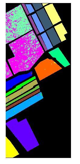
You can also read