IAB-DISCUSSION PAPER 3|2021 The effects of private versus public health insurance on health and labor market outcomes - Doku.iab .

v

IAB-DISCUSSION PAPER
Articles on labour market issues

3|2021 The effects of private versus public health
insurance on health and labor market outcomes
Christine Dauth

 ISSN 2195-2663

The effects of private versus public health
insurance on health and labor market
outcomes

Christine Dauth (IAB)

Mit der Reihe „IAB-Discussion Paper“ will das Forschungsinstitut der Bundesagentur für Arbeit
den Dialog mit der externen Wissenschaft intensivieren. Durch die rasche Verbreitung von For-
schungsergebnissen über das Internet soll noch vor Drucklegung Kritik angeregt und Qualität ge-
sichert werden.

The “IAB Discussion Paper” is published by the research institute of the German Federal Employ-
ment Agency in order to intensify the dialogue with the scientific community. The prompt publi-
cation of the latest research results via the internet intends to stimulate criticism and to ensure
research quality at an early stage before printing.

Contents
1 Introduction ....................................................................................................................... 7

2 Related literature ............................................................................................................... 8

3 Institutional background of health insurance in Germany .................................................. 9

4 Data and sample restriction.............................................................................................. 10

5 Empirical approach .......................................................................................................... 14
 5.1 Identification strategy ....................................................................................................... 14
 5.2 Assumptions ....................................................................................................................... 15

6 Causal estimates of private health insurance on health and employment ........................ 20
 6.1 First stage results ............................................................................................................... 20
 6.2 Reduced form results ......................................................................................................... 22
 6.3 Two stage least squares results......................................................................................... 23
 6.4 Sensitivity Checks .............................................................................................................. 25

7 Summary and conclusion ................................................................................................. 27

Figures
Figure 1: Regression discontinuity plots of monthly earnings for predetermined
 covariates ................................................................................................................ 19
Figure 2: Density test of the forcing variable around the cutoff ........................................... 20
Figure 3: First stage effects: bin scatter plots of private health insurance (PHI) rates
 below and above the compulsory insurance threshold ........................................ 21
Figure 4: Reduced form estimates for the impact of private health insurance (PHI) on
 … over nine years .................................................................................................... 23

Tables
Table 1: Mean sample statistics for workers in private health insurance (PHI) and
 public statutory health insurance (SHI) in base year t ∈ [2003,2006] ................... 13
Table 2: Mean sample statistics for workers above and below the compulsory
 insurance threshold ................................................................................................ 17
Table 3: OLS and 2SLS estimates of private health insurance (PHI) on health and labor
 market outcomes .................................................................................................... 21
Table 4: OLS and 2SLS estimates with control variables of private health insurance
 (PHI) on health and labor market outcomes.......................................................... 24
Table 5: OLS and 2SLS estimates with control variables of private health insurance
 (PHI) and labor market outcomes over 9 years ..................................................... 26

Abstract
Among health care systems with both public and private elements (such as in the US and Ger-
many), an important question is whether the type of health insurance exerts an impact on workers’
careers. We exploit the unique German case of a two-tier health care system to analyze whether
opting out of public statutory health insurance and into private health insurance affects the spe-
cific health and employment outcomes of employed workers over a period of nine years. We ex-
ploit administrative registers and apply a fuzzy regression discontinuity design. We do not find any
evidence that the type of health insurance affects employed workers’ outcomes in the medium or
long run. This suggests that even though private health insurance entails more comfortable
healthcare conditions, public health insurance does not come with heavy health impairments or
detrimental employment outcomes.

Zusammenfassung
In Gesundheitssystemen mit gesetzlichen und privaten Krankenversicherungen (so wie beispiels-
weise in den USA oder in Deutschland), stellt sich die Frage, ob die Art der Krankenversicherung
die Arbeitsmarktkarrieren der Versicherten beeinflusst. Wir untersuchen, ob der Wechsel von der
gesetzlichen in die private Krankenversicherung bestimmte Gesundheits- und Beschäftigungsva-
riablen über einen Zeitraum von neun Jahren beeinflusst. Wir nutzen administrative Prozessdaten
und verwenden ein Fuzzy Regression Discontinuity Design um kausale Effekte zu identifizieren. Wir
finden keinerlei Hinweise auf einen mittel- oder langfristigen Einfluss der Art der Krankenversiche-
rung auf lange Krankheitsepisoden oder den Arbeitsmarkterfolg von Beschäftigten. Dies deutet
darauf hin, dass eine Mitgliedschaft in der privaten Krankenversicherung zwar mit mehr Annehm-
lichkeiten verbunden ist, aber nicht mit gravierenden Nachteilen bei der Gesundheit oder dem Ar-
beitsmarkterfolg.

JEL classification
I13, J21, J30

Keywords
Employment, fuzzy RDD, health instrumental variables, labor market outcomes, private health in-
surance, public health insurance

IAB-Discussion Paper 3|2021 5

Acknowledgements
I thank Wolfgang Dauth, Caroline Hiesinger, Simon Janssen, Gesine Stephan and the conference
participants of the 2019 European Society of Population Economics conference for their helpful
comments and suggestions. Special thanks to the DIM department of the Institute for Employment
Research (IAB) for providing the data.

IAB-Discussion Paper 3|2021 6

1 Introduction
Health care systems around the globe are very differently organized and therefore hard to com-
pare. Most European systems provide universal public primary health care with complementary
health care coverage from private insurers (Paris et al. 2010, Tuohy et al. 2004). The United States,
by contrast, organizes health care predominantly privately, except for older individuals (Medicare)
and deprived workers (Medicaid) (Brown 2003). Whether individuals’ health and employment out-
comes depend on the institutional organization of health care is uncertain.
The German case provides an ideal setup to explore whether private or public health insurance
affects worker outcomes differently. Health care in Germany is organized in a two-tier system. Pri-
vate health insurance (PHI) is open only to specific workers, i.e., government officials, self-em-
ployed workers, and employees with high incomes. The remaining 87 percent of all workers in the
labor force have public statutory health insurance (SHI) (Statistisches Bundesamt 2016). 1 One im-
portant difference between private and public health insurance is that private insurance compa-
nies compensate physicians more generously than public health insurance funds (Walendzik et al.
2008). 2 PHI companies reimburse physicians approximately 2.3 times higher on average for the
same type of treatment, reimburse longer time slots to treat patients, reimburse more consulta-
tions for the same illness, and reimburse a larger set of health care services as well as more expen-
sive medication and therapies (Stauder and Kossow, 2017). Consequently, physicians treat pa-
tients with SHI and PHI differently. For example, SHI patients wait approximately three times as
long for outpatient appointments than PHI patients (Lüngen et al. 2008) and approximately 19 per-
cent longer for appointments at acute care hospitals (Kuchinke et al. 2009).
The relationship between the type of health insurance and the use of health care services in Ger-
many is uncertain. Some studies do not find any correlation between the type of health insurance
and the number of appointments at hospitals or physicians (Geil et al. 1997; Pohlmeier and Ulrich
1995; Riphahn et al. 2003). Others find that workers with PHI visit the doctor more often than SHI
members (Jürges 2009) and that privately insured men visit specialists more often than publicly
insured men (Gruber and Kiesel 2010).
The purpose of this paper is to analyze whether the type of health insurance affects employed
workers’ health and labor market outcomes over a period of nine years. We assume that the main
underlying mechanism is differences in patients’ treatment by physicians, who respond to the fi-
nancial incentives that emerge from differences in payment generosity. Potentially resulting
health effects will subsequently reflect upon employment, because bad health lowers employ-
ment probability (Frijters et al., 2014; García-Gómez et al. 2013, Zimmer 2013) and earnings (Halla
and Zweimüller 2013). To identify causal effects, we apply a fuzzy regression discontinuity design
and exploit that in Germany, employees’ earnings must exceed a certain income threshold for
them to become eligible to opt out of public SHI. This allows us to control for the selection of spe-
cific worker types in PHI. Moreover, we exploit extremely rich and precise register data covering all
German employees.

1
 Among employees, i.e., excluding civil servants and self-employed workers, 96 percent have SHI and four percent have PHI.
2
 This is similar to the US, where private insurers reimburse at higher rates than Medicaid (Alexander and Schnell, 2019).

IAB-Discussion Paper 3|2021 7

In sum, we find no evidence of any impact of PHI on employees’ long-term health status or mor-
tality or on their cumulative employment or job position. Thus, PHI seems to provide better amen-
ities for insurance users but does not directly affect workers’ health status or career.
The paper is organized as follows: Section 2 summarizes the related literature and section 3 the
institutional background. Section 4 describes the data and section 5 the methodological ap-
proach. Section 6 presents the results, and section 7 concludes.

2 Related literature
Because there is no universal health insurance coverage in the US, a considerable amount of liter-
ature focuses on whether health insurance coverage itself increases the use of health care services
and improves the health outcomes of insured individuals. On the one hand, workers covered by
health insurance potentially have better access to information about the risks of unhealthy behav-
ior and are more likely to receive ambulatory and inpatient care (Davis and Rowland 1983). On the
other hand, insured workers might increase their risky behavior due to moral hazard. Moreover,
workers are treated for emergency conditions also when non-insured. In sum, findings regarding
the impact of health insurance coverage on health outcomes and mortality depend on the context
and are ambiguous (see Goldin et al. 2021). However, several important studies based on random-
ized controlled trials and natural experiments have found a positive impact of health insurance
coverage on the use of health services, health outcomes, and mortality (Baicker et al. 2013, Card
et al. 2008, Currie and Gruber 1996a/b, Finkelstein et al. 2012, Sommers et al. 2012).
A smaller body of literature deals with disparities in reimbursement generosity and their role in
differences in patients’ treatment and their health outcomes. It has conclusively been shown that
reimbursement rates drive physician behavior. The most recent literature for the US is predomi-
nantly concerned with comparing workers publicly insured by Medicaid and workers privately in-
sured by their employer. Higher Medicaid reimbursement rates improve access to health care, in-
crease self-reported health, and reduce school absenteeism (Alexander and Schnell, 2019). More-
over, publicly insured children are less likely to be admitted to hospitals than privately insured
children, especially during flu season, when hospital beds are in high demand. However, this does
not seem to affect children’s health outcomes, which indicates that in general, children might be
overtreated (Alexander and Currie 2017). The findings from Gruber et al. (1999) provide additional
supportive evidence that higher relative reimbursement rates might coincide with needlessly in-
tensive treatment of patients. The higher fee differentials between cesarean and normal childbirth
in Medicaid than in private health insurance explain over half of the difference between Medicaid
and private cesarean delivery rates.
In addition to the literature on Medicaid, Clemens and Gottlieb (2014) examine exogenous shocks
to Medicare physician payments. They find that a two percent increase in reimbursement rates
leads to a three percent increase in health care services. While relatively elective services show the
strongest response, less discretionary services respond little to the change in payment rates. Fo-
cusing solely on private health insurance, Coey (2015) shows that physicians choose more costly

IAB-Discussion Paper 3|2021 8

heart attack treatments when insurance plans reimburse them at higher rates than alternative
treatments.
While Medicaid covers only workers with low income, German workers covered by SHI have char-
acteristics that are representative of the average population. Therefore, the German case is ideal
to verify whether the type of health insurance affects individuals’ health outcomes in the long run
with a different, more representative subset of workers.
To date, three studies have analyzed the causal health effects of the German two-tier system. Ap-
plying a fuzzy regression discontinuity design to survey data, Hullegie and Klein (2010) show that
the type of insurance does not affect the number of nights stayed in a hospital. However, PHI mem-
bers less often consult a physician and report better health. Petilliot (2017) focuses on young indi-
viduals still in the school system. He assumes that for them, the type of health insurance is exoge-
nous, because most students’ parents decide on the type of health insurance at birth. Using survey
data, he does not find any differences in self-reported health status or health satisfaction between
those with PHI and those with SHI. Stauder and Kossow (2017) apply an individual fixed effects
approach to survey data. They find that with every year on PHI, workers can significantly improve
their physical component summary scale score compared to workers on SHI. Together, the previ-
ous studies report differing findings regarding the effect of insurance type on health outcomes,
which is certainly related to differences in data, methodologies, and samples.
Our study makes important contributions to the literature. First, compared to the existing studies
that evaluate the German setting and rely predominantly on survey data, we are the first to exploit
comprehensive register data that authorities systematically collect to calculate employees’ social
security contributions. We can draw on data from all German employees at the daily level. Second,
we do not rely on self-reported but objective health measures. The register data allow us to iden-
tify when workers interrupt or end employment due to severe sickness or death. Third, we close a
gap in the literature and analyze how PHI affects workers’ employment outcomes via health sta-
tus. Assuming that health is an important driver of workers’ careers, we analyze how the insurance
type affects cumulative employment and workers’ job position. With US data, this is hardly feasi-
ble, as it is the employer that commonly organizes private health insurance in the US. Thus, health
care coverage itself is an important incentive to stay employed, irrespective of health status.
Fourth, we follow individuals over a period of nine years, and this study is therefore unique in pre-
senting long-term evidence.

3 Institutional background of health
insurance in Germany
In Germany, SHI is mandatory for employees whose regular earnings fall below the Compulsory
Insurance Threshold (CIT). In 2019, the annual CIT was 60,750 euros. As the average income from
work was 47,928 euros 3, this implies that only high-earning employees can choose between SHI

3
 Federal Statistical Office 2021, https://www.destatis.de/DE/Themen/Arbeit/Verdienste/Verdienste-Verdienstunterschiede/ver-
dienste-branchen.html.

IAB-Discussion Paper 3|2021 9

and PHI. Regular earnings comprise monthly earnings plus regular bonuses. When a worker’s reg-
ular earnings exceed the monthly CIT and will also exceed the threshold the following year, he can
opt out of SHI and buy PHI at the beginning of the new year.
In addition to differences in eligibility, PHI and SHI differ with respect to the insurance premiums
workers need to pay and with respect to the insurance benefits. The 110 German nonprofit health
insurance funds that supply SHI generally offer the same standard package of health care services
with slight deviations (Gesetzliche Krankenversicherung (GKV)-Spitzenverband 2018). By contrast,
private for-profit health insurance companies usually offer different combinations of health care
services at different prices. The cheapest package must cover the same services as SHI at the same
prices.
Health premiums under SHI depend on labor earnings. This implies that up to a certain earnings
ceiling (56,250 euros in 2019), the premium amounts to approximately 15 percent of a worker’s
earnings. By contrast, health premiums under PHI are risk-related. In both cases, the employer
covers approximately half of the health premium. Private insurers classify workers and set the pre-
miums when workers enroll in PHI. The most relevant risk factors are age and health condition
and, before 2013, gender (women paid more). Health contracts are life-long, and private insurers
can neither adjust nor cancel the contract in response to health shocks once they have closed a
health contract.
When individuals choose between SHI and PHI, the relative price matters. Particularly for young,
healthy and high-earning males, PHI offers better health care services at lower premiums. Indeed,
the literature has largely confirmed that workers with PHI are younger, have higher earnings and
are more likely to be male. This selection is the consequence of better risks opting out of SHI (Bün-
nings and Tauchmann 2015) and worse risks opting back into SHI (Grunow and Nuscheler 2014).
However, Panthöfer (2016) shows that relative prices explain only approximately one third of the
selection into PHI. Polyakova (2016) finds only limited evidence for better risks enrolling in PHI.
She argues that individuals with a preference for convenience (shorter appointment waiting times,
better hospital rooms) in particular chose PHI.
The coexistence of both systems has repeatedly been the focus of public debate because many
consider it unjust. PHI is open only to specific workers, i.e., government officials, self-employed
workers, and employees with high earnings. Moreover, PHI attracts healthier workers because the
insurance premiums are health-dependent. This lowers the costs and premiums in PHI and weak-
ens the principle of solidarity in public SHI.

4 Data and sample restriction
We exploit administrative records provided by the Institute for Employment Research of the Ger-
man Federal Employment Agency. These data comprise information on all employed workers,
such as the date and duration of employment, earnings, individual characteristics, and job char-
acteristics. Because all of this information is process‐generated, it has daily precision and is highly
reliable (Antoni et al. 2019).

IAB-Discussion Paper 3|2021 10

Our analysis relies on the full sample of the Employment History (BeH) dataset, which comprises
employment data for all German employees. We focus on workers liable to social security contri-
butions. To identify employees with SHI or PHI, we rely on a key that identifies to which of the four
social security insurances workers contribute, i.e., health insurance, nursing insurance, pension
insurance, or unemployment insurance. Workers with full PHI contribute to pension and unem-
ployment insurance but do not contribute to health and nursing insurance. Workers with SHI con-
tribute to all four insurances.
We construct a yearly panel for the years 2000 to 2017. Earlier observations do not report contri-
butions to the social security insurances. We focus on workers whose yearly gross earnings vary
closely around the CIT by a maximum of 2,500 euros between 2003 and 2006. In January 2003, the
government substantially raised the CIT to increase the proportion of workers with SHI and to se-
cure SHI revenue (Verband der privaten Krankenversicherung 2004). This implies that between
2000 and 2002, the CIT was much lower, which is why we exclude these years from our observation
period. We also exclude the years after 2006 because between 2007 and 2010, the eligibility criteria
changed again: workers had to cross the CIT for at least three years in a row to qualify for PHI.
Annual earnings are the key determinant for workers to become eligible for PHI. Therefore, we
condition on workers who have been continuously employed and liable to social security contri-
butions for the three years before we measure annual earnings. Conditioning on stable employ-
ment for a period this long should exclude workers with serious health limitations. Unhealthy
workers might sooner or later be forced to register as disabled and interrupt their employment
spell. Moreover, only healthy workers are potential compliers who might opt out of SHI once their
earnings exceed the CIT. As noted above, health status, in addition to age and gender, is an im-
portant determinant for insurance premiums when workers close a health insurance contract with
a private insurance company. We furthermore focus on workers between age 25 and 45 in the years
2003 to 2006 because the majority of workers opt out of SHI within this age span. We limit the
analyses to men because for women, we cannot disentangle maternity benefits from sickness ben-
efits.
We are interested in workers who have not yet taken the opportunity to opt out of SHI. Conse-
quently, we condition our analyses on workers who were not privately insured in the three preced-
ing years. Then, in base year t ∈ [2003,2006], some of these workers’ earnings exceed the CIT, and
they can opt out of SHI. We measure the type of health insurance in year t + 2 ∈ [2005,2008], i.e.,
two years after we measure workers’ earnings relative to the CIT. Therefore, we account for the
time it might take workers to decide on PHI and to complete the administrative process to change
their health insurance type.
We are able to observe all workers’ outcomes for up to nine years. The register data allow us to
measure both health effects and employment effects. Regarding employment outcomes, we want
to know whether the type of health insurance affects the cumulative days workers are employed
and subject to social security contributions and the cumulative days they are no longer in the so-
cial security registers. The latter indicate periods in which workers left the labor force, became
self-employed or entered civil service. If employees plan to change to self-employment or civil ser-
vice in the future, they might be more likely to opt into PHI while still employed. Exploring the
“nonregistered” outcome, we can investigate whether such anticipation is relevant in our setting.
Moreover, the data contain information on workers’ job position, i.e., if workers are unskilled,

IAB-Discussion Paper 3|2021 11

skilled, specialists, or experts. Another outcome is therefore the probability that workers have the
job position of a specialist or expert after five and nine years.
Regarding health outcomes, we can identify whether workers end or interrupt their employment
spell due to sickness lasting several weeks or due to death. The reason is that employers have to
report to the social security authorities if workers interrupt employment and no longer receive a
salary. There are different keys to describe why workers no longer receive a salary. We code an
employment termination due to death if employers report key 49 (deregistration due to death).
We code an employment interruption due to sickness if employers report that an employment
spell ended due to key 51. This key most commonly implies that workers receive sickness benefits
or maternity benefits (relevant to women only). Note, however, that this allows us to identify only
those sickness spells with a minimum duration of 10 weeks. The employer must not report shorter
sickness periods. 4 Thus, the interruptions we observe imply severe health problems, which are
more likely to affect future employment outcomes than sickness periods of only a few days. More-
over, observing outcomes for employed workers, but not for workers who have already left the
labor force implies that we probably observe only a few mortality outcomes, because it is likely for
very sick people to drop out of the labor force when they face death.
Control variables are measured in January of base year t. Table 1 reports some sample statistics.

4
 If workers report sick to the employer for several weeks, usually, the employer must continue salary payments for the first six
weeks of the sickness. Starting in week seven, the employer stops paying the salary, and health insurance disburses sickness
benefits. Employers report an employment interruption due to sickness benefits only if sickness benefits are paid for a full cal-
endar month and the employer therefore must not pay the salary for a full calendar month.

IAB-Discussion Paper 3|2021 12

Table 1: Mean sample statistics for workers in private health insurance (PHI) and public statutory
health insurance (SHI) in base year t ∈ [2003,2006]
 PHI SHI difference p-value
PHI 1.00 0.00 1.00 0.00
Age 34.48 37.54 -3.06 0.00
Age squared 1212.36 1433.61 -221.25 0.00
Foreign 0.03 0.06 -0.03 0.00
Part-time 0.01 0.01 0.00 0.48
Job level: unknown 0.00 0.01 0.00 0.00
Job level: unskilled 0.00 0.01 0.00 0.00
Job level: skilled 0.52 0.67 -0.16 0.00
Job level: specialist 0.21 0.16 0.05 0.00
Job level: expert 0.27 0.15 0.12 0.00
Without vocational training 0.01 0.05 -0.04 0.00
In-company voc. training/traineeship/external (on-school) voc. training 0.51 0.69 -0.18 0.00
Technical school (voc. training) 0.02 0.01 0.01 0.00
Technical school (advanced voc. training) 0.13 0.07 0.06 0.00
University of applied sciences (FH) 0.11 0.07 0.04 0.00
University 0.14 0.07 0.08 0.00
Vocational training info missing 0.07 0.04 0.03 0.00
Farmers (agriculture, horticulture, forestry), animal breeders, fishermen 0.00 0.00 0.00 0.01
Miners, mineral quarries 0.00 0.00 0.00 0.00
Stone preparers, building material makers 0.00 0.00 0.00 0.18
Ceramics workers, glass makers 0.00 0.00 0.00 0.02
Chemical workers, plastics processors 0.01 0.03 -0.03 0.00
Paper makers, printers 0.01 0.01 -0.01 0.00
Wood preparers, wood product makers and related occupations 0.00 0.00 0.00 0.01
Metal producers, metal molders, metal workers 0.01 0.05 -0.04 0.00
Locksmiths, mechanics and related occupations 0.04 0.13 -0.09 0.00
Electricians 0.02 0.05 -0.03 0.00
Assemblers and metal workers (no further specification) 0.01 0.04 -0.03 0.00
Textile makers, processers and finishers 0.00 0.00 0.00 0.19
Leather makers, leather and fell processers 0.00 0.00 0.00 0.07
Occupation in food production and processing 0.00 0.01 0.00 0.02
Building occupations 0.01 0.01 0.00 0.00
Building finishers, room equippers, upholsterers 0.00 0.00 0.00 0.00
Carpenter, model maker 0.00 0.00 0.00 0.00
Painters, lacquerers and related occupations 0.00 0.01 -0.01 0.00
Goods examiners, dispatchers 0.01 0.01 -0.01 0.00
Assistants (no further specification) 0.00 0.01 0.00 0.00
Machinists and related occupations 0.00 0.02 -0.02 0.00
Engineers, chemists, physicists, mathematicians 0.11 0.06 0.06 0.00
Technicians, technical specialists 0.14 0.14 0.00 0.11
Wholesale and retail traders 0.09 0.04 0.04 0.00
Service agents and related occupations 0.15 0.07 0.08 0.00
Transport and communication occupations 0.02 0.04 -0.02 0.00
Management, administration, and office occupations 0.30 0.19 0.11 0.00
Safety, security, and legal occupations 0.01 0.01 -0.01 0.00
Journalists, interpreters, librarians, artists 0.01 0.01 0.00 0.00

IAB-Discussion Paper 3|2021 13

PHI SHI difference p-value
Health occupations 0.00 0.01 -0.01 0.00
Social and educational occupations, occupations in humanities or science (no
 0.04 0.03 0.00 0.00
further specification)
Other service occupations 0.00 0.01 0.00 0.00
Workforce not further specified 0.00 0.00 0.00 0.76
Disabled, in rehabilitation 0.00 0.00 0.00 0.61
Occupation missing 0.00 0.00 0.00 0.77
Cumulative days receiving welfare benefits in base year t 0.00 0.03 -0.03 0.08
Number of welfare benefit spells in base year t 0.00 0.00 0.00 0.08
Aggregate earnings in three years prior to base year t 148508.44 146358.03 2150.41 0.00
Cumulative tenure with interruption in three years prior to base year t 927.55 988.34 -60.80 0.00
Cumulative tenure without interruption in three years prior to base year t 923.08 985.50 -62.43 0.00
Number of recalls in three years prior to base year t 0.01 0.01 0.00 0.00
Average number of establishments in three years prior to base year t 1.35 1.21 0.14 0.00
Average daily wage in three years prior to base year t 117.10 117.88 -0.78 0.00
State missing 0.00 0.00 0.00 0.88
State Schleswig-Holstein 0.02 0.02 0.00 0.00
State Hamburg 0.03 0.03 0.00 0.01
State Niedersachsen 0.07 0.09 -0.02 0.00
State Bremen 0.01 0.02 -0.01 0.00
State Nordrhein-Westfalen 0.22 0.24 -0.02 0.00
State Hessen 0.10 0.09 0.00 0.35
State Rheinland-Pfalz 0.05 0.05 0.00 0.04
State Baden-Württemberg 0.19 0.20 -0.02 0.00
State Bayern 0.18 0.17 0.01 0.00
State Saarland 0.01 0.02 -0.01 0.00
State Berlin 0.04 0.03 0.02 0.00
State Brandenburg 0.01 0.01 0.01 0.00
State Mecklenburg-Vorpommern 0.01 0.01 0.00 0.00
State Sachsen 0.04 0.02 0.02 0.00
State Sachsen-Anhalt 0.01 0.01 0.01 0.00
State Thüringen 0.01 0.01 0.01 0.00
Base year t=2003 0.41 0.26 0.15 0.00
Base year t=2004 0.24 0.25 -0.02 0.00
Base year t=2005 0.23 0.24 -0.02 0.00
Base year t=2006 0.12 0.24 -0.12 0.00
N 28068 1268945
Source: BeH V10.02.01. Own calculations.

5 Empirical approach
5.1 Identification strategy
The main challenge when analyzing the causal effects of private health insurance on workers’ out-
comes is that specific types of workers select into private health insurance. Privately insured em-
ployees have higher earnings by design, which again correlate with better health and better future

IAB-Discussion Paper 3|2021 14

labor market outcomes (e.g., Zagorsky and Smith 2020). However, we do not observe data on in-
dividuals’ work motivation or health status or information such as health awareness, eating hab-
its, or drug consumption. To avoid omitted variable bias, we therefore estimate the effect of PHI
using a fuzzy regression discontinuity design (fuzzy RDD), assuming that characteristics are similar
for individuals close around the cutoff point (Hahn et al. 2001; Imbens and Lemieux 2008).
The possibility of opting out of SHI and buying into PHI is a discontinuous function of a worker’s
earnings. If his regular earnings exceed the CIT, he has the ability to opt out of SHI and buy into
PHI. If his regular earnings are below the CIT, he must use SHI. Unlike in a sharp RDD setting, the
cutoff does not deterministically define whether workers have PHI. On the one hand, not all indi-
viduals who cross the CIT in year t opt out of SHI at year t + 2 (never-takers). On the other hand,
some individuals’ earnings might still be below the CIT in year t, but they have opted into PHI at
year t + 2 nevertheless (always-takers).
In our empirical approach, first, we compare the probability of having PHI in year t + 2 for workers
either slightly below or slightly above the CIT in year t. Second, we compare the long-term out-
comes at t + 7 and t + 11, i.e., five and nine years after we observe the health insurance status of
workers either slightly below or slightly above the CIT in year t. Implementing this, in an initial step,
we estimate the following first-stage equation:
 PHIit+2 = 0 + 1 Ι (earningsit ≥ C T ) + 2 Ι (earningsit ≥ C T ) ∗ earningsit + (1)
 �
 + 3 earningsit [+ 4 Xit ] + it = PHI i +2 + it .

PHIit+2 is the treatment indicator, which takes the value 1 for individual i who buys into PHI in year
t + 2. earningsit comprises a worker’s annual earnings from employed work in year t. Xit is a vector
of individual characteristics–such as age, vocational degree, occupation, and employment history
in the previous three years–and regional controls for the 16 states. We include these controls to
increase the precision of the estimates.
For the reduced form equation, we estimate
 Yit+2+9 = 0 + 1 Ι (earningsit ≥ C T ) + 2 Ι (earningsit ≥ C T ) ∗ earningsit + (2)
 � + it
 + 3 earningsit [+ 4 Xit ] + it = Yi +2+9
With Yit+2+9 as individual i’s health or employment outcome (such as cumulative employment and
earnings). 1 identifies the discrete change in subsequent health and labor market outcomes for
workers earning above the CIT, controlling for their earnings and other observable characteristics.
To obtain our fuzzy RDD estimates, we apply two-stage least squares (2SLS) estimation. Thus, for
the second stage, we estimate
 �
 Yit+2+9 = 0 + 1 PHI i +2 + 2 earningsit + 3 Xit + it . (3)
γ1 identifies the local average treatment effect (LATE) for compliers. Compliers are workers whose
regular earnings exceed the CIT in year t, who have not had PHI in the preceding three years, and
who in year t + 2 have the opportunity to opt out of SHI.

5.2 Assumptions
The validity of this approach hinges on several assumptions (Hahn et al. 2001; Imbens and Lemieux
2008, Lee and Lemieux 2010). First, our setting must meet the monotonicity assumption. This im-
plies that we must exclude the possibility that some workers are more likely to buy PHI once they
cross the threshold, while others reject PHI once they cross the threshold. The assumption holds

IAB-Discussion Paper 3|2021 15

by design, because workers below the CIT are generally ineligible for PHI. Moreover, the data
clearly show that the probability of buying into PHI increases with earnings (see Figure 3). 5
Second, the exclusion restriction requires that earnings above the cutoff affect outcomes only by
increasing the probability of buying into PHI, not directly. This assumption should hold because
we chose small bandwidths around the cutoff and therefore look at workers whose annual earn-
ings differ by small amounts. It is unlikely that these small differences influence employment or
health outcomes differently.
Third, individuals must be unable to precisely control earnings around the threshold (Lee and
Lemieux 2010). On the one hand, workers with a strong preference for PHI might try to increase
their earnings to exceed the CIT. However, employed workers usually have limited opportunities
to influence their regular earnings. Even if workers qualify for a one-time bonus, social insurance
will not take into account this type of irregular income. On the other hand, workers with families
are more likely to continue to use SHI (Bünnings and Tauchmann, 2015). The reason is that without
any additional costs, SHI, unlike PHI, uniquely covers the health insurance for an employee’s chil-
dren and nonemployed spouse. However, SHI is available for all employees, and thus, workers
with families have no incentive to manipulate their earnings.
If this assumption holds, both observable and unobservable characteristics should be balanced
around the threshold. Table 2 presents the observable characteristics of workers just above and
below the threshold. The differences in characteristics are statistically significant in most cases,
but often, the economic importance is negligible. Additionally, Figure 1 displays the distribution
around the cutoff of the selected observable characteristics age, foreign origin, expert job status,
secondary education with a vocational degree, earnings over the three years before t, and tenure
in days over the three years before t. Overall, there are no statistically significant jumps at the cut-
off. However, Figure 1 c) and d), which capture workers’ qualifications, seem somewhat discontin-
uous. To rule out any unnecessary bias, we will condition our main analyses on observable char-
acteristics, in particular for measures of qualifications.

5
 In Figure 3, some observations below the threshold have PHI. The reason is that we measure the running variable in year t,
while we measure PHI in year t+2, i.e., two years later. Thus, there are workers whose earnings are below the threshold in year t
but whose earnings have crossed the threshold in year t+2, making them eligible for PHI in year t+2.

IAB-Discussion Paper 3|2021 16

Table 2: Mean sample statistics for workers above and below the compulsory insurance threshold

 above CIT below CIT difference p-value
PHI 0.03 0.01 0.02 0.00
Age 37.54 37.42 0.12 0.00
Age squared 1433.38 1425.22 8.15 0.00
Foreign 0.05 0.06 -0.01 0.00
Part-time 0.01 0.01 0.00 0.00
Job level: unknown 0.01 0.01 0.00 0.00
Job level: unskilled 0.01 0.01 0.00 0.00
Job level: skilled 0.64 0.70 -0.06 0.00
Job level: specialist 0.18 0.15 0.03 0.00
Job level: expert 0.17 0.14 0.03 0.00
Without vocational training 0.04 0.06 -0.01 0.00
In-company voc. training/traineeship/external (on-school) voc. training 0.67 0.70 -0.04 0.00
Technical school (voc. training) 0.01 0.01 0.00 0.00
Technical school (advanced voc. training) 0.08 0.07 0.01 0.00
University of applied sciences (FH) 0.08 0.06 0.02 0.00
University 0.08 0.06 0.02 0.00
Vocational training info missing 0.05 0.04 0.00 0.00
Farmers (agriculture, horticulture, forestry), animal breeders, fishermen 0.00 0.00 0.00 0.00
Miners, mineral quarries 0.00 0.00 0.00 0.00
Stone preparers, building material makers 0.00 0.00 0.00 0.00
Ceramics workers, glass makers 0.00 0.00 0.00 0.00
Chemical workers, plastics processors 0.03 0.04 -0.01 0.00
Paper makers, printers 0.01 0.01 0.00 0.00
Wood preparers, wood product makers and related occupations 0.00 0.00 0.00 0.00
Metal producers, metal molders, metal workers 0.04 0.05 -0.01 0.00
Locksmiths, mechanics and related occupations 0.12 0.14 -0.02 0.00
Electricians 0.05 0.05 0.00 0.00
Assemblers and metal workers (no further specification) 0.03 0.04 -0.01 0.00
Textile makers, processers and finishers 0.00 0.00 0.00 0.01
Leather makers, leather and fell processers 0.00 0.00 0.00 0.56
Occupation in food production and processing 0.01 0.01 0.00 0.00
Building occupations 0.01 0.01 0.00 0.00
Building finishers, room equippers, upholsterers 0.00 0.00 0.00 0.00
Carpenter, model maker 0.00 0.00 0.00 0.00
Painters, lacquerers and related occupations 0.01 0.01 0.00 0.00
Goods examiners, dispatchers 0.01 0.02 0.00 0.00
Assistants (no further specification) 0.00 0.01 0.00 0.00
Machinists and related occupations 0.02 0.02 0.00 0.00
Engineers, chemists, physicists, mathematicians 0.07 0.05 0.02 0.00
Technicians, technical specialists 0.15 0.13 0.03 0.00
Wholesale and retail traders 0.05 0.04 0.01 0.00
Service agents and related occupations 0.08 0.07 0.01 0.00
Transport and communication occupations 0.03 0.04 -0.01 0.00
Management, administration, and office occupations 0.20 0.18 0.03 0.00
Safety, security, and legal occupations 0.01 0.01 0.00 0.00
Journalists, interpreters, librarians, artists 0.01 0.01 0.00 0.00

IAB-Discussion Paper 3|2021 17

above CIT below CIT difference p-value
Health occupations 0.01 0.01 0.00 0.00
Social and educational occupations, occupations in humanities or science (no fur-
 0.03 0.04 0.00 0.05
ther specification)
Other service occupations 0.00 0.01 0.00 0.00
Workforce not further specified 0.00 0.00 0.00 0.81
Disabled, in rehabilitation 0.00 0.00 0.00 0.18
Occupation missing 0.00 0.00 0.00 0.81
Cumulative days receiving welfare benefits in base year t 0.02 0.03 -0.01 0.01
Number of welfare benefit spells in base year t 0.00 0.00 0.00 0.08
Aggregate earnings in three years prior to base year t 150668.84 143031.56 7637.29 0.00
Cumulative tenure with interruption in three years prior to base year t 982.36 990.72 -8.37 0.00
Cumulative tenure without interruption in three years prior to base year t 979.34 987.96 -8.61 0.00
Number of recalls in three years prior to base year t 0.01 0.01 0.00 0.00
Average number of establishments in three years prior to base year t 1.22 1.20 0.02 0.00
Average daily wage in three years prior to base year t 120.78 115.55 5.23 0.00
State missing 0.00 0.00 0.00 0.26
State Schleswig-Holstein 0.02 0.02 0.00 0.00
State Hamburg 0.04 0.03 0.00 0.00
State Niedersachsen 0.09 0.09 0.00 0.00
State Bremen 0.01 0.02 0.00 0.00
State Nordrhein-Westfalen 0.24 0.24 0.00 0.00
State Hessen 0.10 0.09 0.00 0.00
State Rheinland-Pfalz 0.05 0.05 0.00 0.00
State Baden-Württemberg 0.20 0.20 0.00 0.00
State Bayern 0.17 0.17 0.00 0.97
State Saarland 0.02 0.02 0.00 0.00
State Berlin 0.03 0.03 0.00 0.00
State Brandenburg 0.01 0.01 0.00 0.85
State Mecklenburg-Vorpommern 0.01 0.01 0.00 0.14
State Sachsen 0.02 0.02 0.00 0.24
State Sachsen-Anhalt 0.01 0.01 0.00 0.54
State Thüringen 0.01 0.01 0.00 0.83
Base year t=2003 0.26 0.26 -0.01 0.00
Base year t=2004 0.25 0.25 0.00 0.05
Base year t=2005 0.24 0.24 0.00 0.28
Base year t=2006 0.24 0.24 0.01 0.00
N 572826 724187
Source: BeH V10.02.01. Own calculations.

IAB-Discussion Paper 3|2021 18

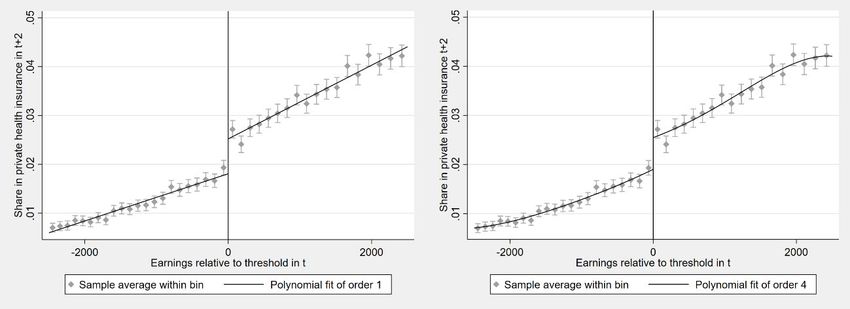
Figure 1: Regression discontinuity plots of monthly earnings for predetermined covariates

Source: BeH V10.02.01. Own calculations.
Notes: The figures show the distribution of exemplary covariates around the compulsory insurance threshold. The solid lines
represent fourth-order global polynomial fitted values following Cattaneo et al. (2019).

Following Cattaneo et al. (2018), we further test whether there is any discontinuity in the density
of the forcing variable (earnings) around the threshold based on a local polynomial density esti-
mator. Figure 2 shows that there is some bunching around the threshold, indicating that the num-
ber of observations just above the threshold is higher than that just below. However, with a t-value
of 0.913 and a p-value of 0.3612, the test does not reject the null hypothesis that the density of

IAB-Discussion Paper 3|2021 19

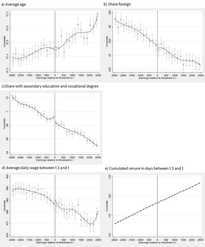
earnings is uniformly distributed around the cutoff. This suggests that there is no statistical evi-
dence of workers’ manipulation of earnings at the threshold.

Figure 2: Density test of the forcing variable around the cutoff

Notes: The left graph displays a histogram of earnings around the cutoff. The right figure displays the density test suggested by
Cattaneo et al. (2018) using a local-polynomial density estimator.
Source: BeH V10.02.01. Own calculations.

6 Causal estimates of private health
insurance on health and employment
In the following, we present the first stage and reduced form results and estimate the 2SLS coeffi-
cients. For a comprehensive overview, the following tables are structured such that we present in
line (1) the coefficients from the OLS regressions for reference and in line (2) the coefficients of
interest from the 2SLS regressions. Line (3) and line (4) present the results from the reduced form
and first stage regressions, respectively.

6.1 First stage results
To apply the fuzzy RDD, we need a valid first stage, i.e., a clear jump in the probability of buying
into PHI at the earnings cutoff. We recode the running variable earnings relative to the CIT with the
value 0 directly at the cutoff. Figure 3 plots the shares of privately insured workers by earnings
around the cutoff using quantile-spaced bins (Calonico et al. 2014). The dots depict the mean val-
ues of both variables within the bins. The solid lines represent first- and fourth-order global poly-
nomial fitted values. As we already know, 96 percent of all employees have SHI, and only 4 percent
have PHI. Given this number, the jump at the cutoff is quite pronounced. Directly below the cutoff,
approximately 1.9 percent of all employees have PHI. These are individuals whose earnings did
not yet exceed the CIT in base year t ∈ [2003,2006] but who had opted out of SHI by t + 2 ∈
[2005,2008]. The share of workers with PHI directly above the cutoff is approximately 2.6 and thus
approximately 40 percent higher. Additionally, line 4 of Table 3 presents the first stage estimates
of an unconditional linear regression and confirms this result: workers above the threshold have a

IAB-Discussion Paper 3|2021 20

0.7-percentage-point higher probability of being privately insured. Moreover, the Kleibergen-Paap
test statistic is above the conventional threshold of 10. Overall, this demonstrates that the share
of PHI workers is discontinuous around the cutoff and that we have a valid first stage with suffi-
cient explanatory power.

Figure 3: First stage effects: bin scatter plots of private health insurance (PHI) rates below and above
the compulsory insurance threshold

Notes: The figures show discontinuities in the share of PHI around the compulsory insurance threshold. The solid lines repre-
sent first- and fourth-order global polynomial fitted values following Cattaneo et al. (2019).
Source: BeH V10.02.01. Own calculations.

Table 3: OLS and 2SLS estimates of private health insurance (PHI) on health and labor market out-
comes
 Sickness Mortality Employment Non-registration Expert level
Over 5 years
1) OLS -0.049*** -0.002*** -58.854*** 61.685*** 0.090***
 (0.001) (0.000) (3.447) (2.981) (0.003)
2) 2SLS -0.151 -0.024 162.082 150.715 0.356**
 (0.119) (0.029) (176.200) (129.326) (0.157)
3) Reduced -0.002* -0.000 2.096 -0.112 0.004***
 form (0.001) (0.00) (1.436) (1.063) (0.001)
Over 9 years
1) OLS -0.078*** -0.003*** -145.044*** 127.524*** 0.129***
 (0.002) (0.00) (6.280) (5.616) (0.003)
2) 2SLS -0.155 0.006 -173.929 384.917 0.183
 (0.153) (0.041) (317.168) (246.340) (0.167)
3) Reduced -0.002* 0.000 2.403 0.090 0.002
 form (0.001) (0.00) (2.587) (2.017) (0.001)
4) First stage: α1 0.007*** 0.007*** 0.007*** 0.007*** 0.007***
 (0.001) (0.001) (0.001) (0.001) (0.001)
 α2 0.000*** 0.00*** 0.000*** 0.000*** 0.000***
 (0) (0) (0) (0) (0)
Kleibergen-Paap 172.428 172.428 172.428 172.428 172.428
N 1297013 1297013 1297013 1297013 1297013
Notes: The outcome sickness (mortality) is the probability that the employer deregisters the worker from employment due to a
sickness of at least ten weeks (or due to death). The outcome variable employment is the cumulative days in fulltime employ-
ment, and the variable non-registration is the cumulative days that the worker is neither employed nor unemployed over the
respective period. The outcome expert level is a dummy variable that is 1 if the worker has reached the highest job level status
five or nine years after we measure the insurance status. The OLS regressions are based on Yit+11 = 0 + 1 PHIit+2 + it . The
2SLS regressions are as in equation (3), the reduced form regressions are as in equation (2), and the first stage regressions are
as in equation (1), all without Xit. Bandwidth: [-2500;2500] euros around cutoff. Significance level: ***p

6.2 Reduced form results
Figure 4 summarizes the mean outcome values within quantile-spaced bins for workers below and
above the contribution threshold. This corresponds to unconditional reduced form estimates.
First, the graphs illustrate the general relationship between earnings and each outcome: the prob-
ability of being sick long-term decreases with earnings, while the probability of having reached the
highest job level, i.e., that of an expert, increases. There is no systematic relation between earnings
and the cumulative days workers are not registered in the social security data or the probability of
being registered dead.
Second, the five graphs of Figure 4 illustrate that employees on both sides of the threshold are
similar in terms of employment stability, time spent nonregistered, or having become an expert.
We also do not find any differences in health outcomes on either side of the cutoff. However, run-
ning unconditional reduced form regressions as in equation (2), we find that workers above the
threshold are approximately 0.2 percentage points less likely to be sick long-term and are 0.4 per-
centage points more likely to have become experts over the following five years (Table 3). Overall,
this indicates that compared to workers with SHI, workers with PHI might profit with respect to
both health and career prospects.

IAB-Discussion Paper 3|2021 22

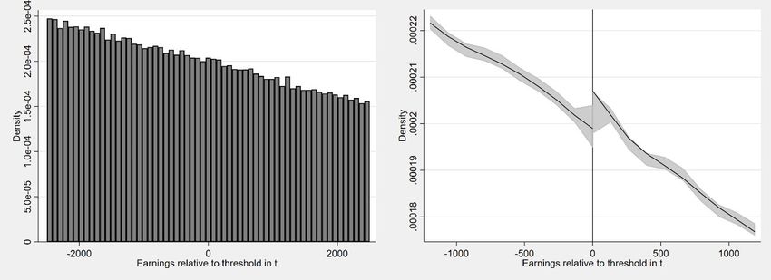
Figure 4: Reduced form estimates for the impact of private health insurance (PHI) on … over nine years

Notes: The figures display potential discontinuities in the outcome variables around the compulsory insurance threshold. The
solid lines represent fourth-order global polynomial fitted values following Cattaneo et al. (2019). The outcome sickness (mor-
tality) is the probability that the employer deregisters the worker from employment due to a sickness of at least ten weeks (or
due to death). The outcome variable employment contains cumulative days in fulltime employment, and the variable non-regis-
tration is the cumulative days that the worker is neither employed nor unemployed over the following nine years. The outcome
job status: expert level is a dummy variable that is 1 if the worker has reached the highest job level status nine years after we
measure insurance status.
Source: BeH V10.02.01. Own calculations.

6.3 Two stage least squares results
We now relate the reduced form findings with our first stage results and present the 2SLS coeffi-
cients. Table 3 presents raw estimates without any control variables for the outcomes over the five

IAB-Discussion Paper 3|2021 23

(nine) years after we measure workers’ health insurance status. The results from the OLS regres-
sions suggest that workers with PHI have an approximately five (eight) percentage point lower
probability of becoming sick long-term and a 0.2 (0.3) percentage point lower probability of mor-
tality. Over five (nine) years, they are approximately nine (thirteen) percentage points more likely
to have reached an expert job level. While they are employed approximately 60 (145) days fewer,
they are nonregistered in the social security data approximately 62 (127) days more. The latter
result might indicate that some workers select into PHI because they anticipate self-employment
or are seeking to become a civil servant. Remember that we observe neither of these latter two
employment types in our data, only that workers dropped out of the registers.
However, conditional on the assumption that workers with anticipations are equally distributed
around the cutoff, we can control for this kind of selection with our 2SLS approach. We find no
causal impact of PHI on health outcomes, employment, or nonregistered days. We do find, how-
ever, that privately insured workers are 35 percentage points more likely to have become experts
after five years. That effect disappears after nine years.
To improve the precision of our estimates and to control for remaining differences in observable
characteristics between workers below and above the threshold, we add a number of control var-
iables. Table 4 shows that adding controls hardly affects the first stage. However, both the coeffi-
cients of the OLS and of the reduced form regressions decrease in most cases. Consequently, we
no longer find any statistically significant differences between workers above and below the CIT
for any outcomes in the reduced form estimations. Thus, all 2SLS coefficients are too imprecisely
estimated to allow for conclusions regarding causal relationships between PHI and health and
employment outcomes.

Table 4: OLS and 2SLS estimates with control variables of private health insurance (PHI) on health and
labor market outcomes
 Sickness Mortality Employment Non-registration Expert level
Over 5 years
1) OLS -0.021*** 0.000 -55.852*** 47.689*** -0.003
 (0.001) (0.00) (3.402) (2.999) (0.002)
2) 2SLS -0.142 -0.025 148.180 138.490 0.095
 (0.120) (0.03) (170.824) (130.325) (0.100)
3) Reduced -0.001 -0.000 1.999 -0.285 0.001
 form (0.001) (0.00) (1.378) (1.058) (0.001)
Over 9 years
1) OLS -0.029*** -0.000*** -127.538*** 104.662*** 0.0390***
 (0.002) (0.00) (6.250) (5.646) (0.003)
2) 2SLS -0.143 0.005 -174.980 350.147 0.005
 (0.153) (0.042) (312.117 (248.122) (0.148)
3) Reduced -0.002 0.000 2.119 -0.228 0.000
 form (0.001) (0.00) (2.517) (2.007) (0.001)
4) First stage: α1 0.007*** 0.007*** 0.007*** 0.007*** 0.007***
 0.001) (0.001) (0.001) (0.001) (0.001)
 α2 0.0000*** 0.0000*** 0.0000*** 0.0000*** 0.0000***
 (0) (0) (0) (0) (0)
Kleibergen-Paap 172.428 172.428 172.428 172.428 172.428
N 1297013 1297013 1297013 1297013 1297013
Notes: Outcome variables as in Table 3. The OLS regressions are based on Yit+11 = 0 + 1 PHIit+2 + it . The 2SLS regressions
are as in equation (3), and the reduced form regressions are as in equation (2). The first stage regressions are as in equation (1).
Controls comprise the variables presented in Table 2. Bandwidth: [-2500;2500] euros around the cutoff.
Significance level: ***p

6.4 Sensitivity Checks
To check if the results above hold when we manipulate the data, we conduct a number of sensi-
tivity checks for the long-term outcomes measured over a period of nine years.
First, we check the sensitivity of the estimates to the choice of bandwidth. We remove observations
at the end points of our sample and focus on workers whose earnings vary by 1,250 and 500 euros
around the CIT separately. The first stage coefficients shrink in both cases, but are both still valid
and highly statistically significant. As above, the reduced form and 2SLS estimates are all statisti-
cally insignificant.
Second, we check the sensitivity of our estimates to observations near the cutoff by applying a
“donut hole” approach (Cattaneo et al. 2019). In the case that workers manipulated their earnings
to become eligible for PHI, potential effects are most likely driven by this group of workers. Assum-
ing that these observations are located close to the threshold, we therefore exclude observations
located 50 and 150 euros around the CIT (see panel 3) and 4) of Table 5, respectively). Overall, our
findings are robust to these checks: we do not find any differences between workers on either side
of the threshold in our reduced form estimates.
In sum, these preliminary findings suggest that even though PHI offers more comfortable health
care conditions, such as shorter waiting times or more intensive treatment by specialists, it does
not affect employed workers’ overall health status, mortality or employment outcomes over the
following nine years.

IAB-Discussion Paper 3|2021 25

Table 5: OLS and 2SLS estimates with control variables of private health insurance (PHI) and labor
market outcomes over 9 years
 Sickness Mortality Employment Non-registration Expert level
Bandwidth 1250 euros
1) OLS -0.031*** 0.0003 -133.985*** 111.842*** 0.0417***
 (0.002) (0.001) (8.308) (7.55) (0.004)
2) 2SLS -0.279 -0.003 -785.699 497.583 0.260
 (0.275) (0.075) (563.394) (445.56) (0.270)
3) Reduced -0.002 -0.0001 -3.305 2.009 0.002
 form (0.002) (0) (3.454) (2.746) (0.002)
4) First stage: α1 0.006*** 0.006*** 0.006*** 0.006*** 0.006***
 (0.001) (0.001) (0.001) (0.001) (0.001)
Kleibergen-Paap 43.679 43.679 43.679 43.679 43.679
N 649554 649554 649554 649554 649554
Bandwidth 500 euros
1) OLS -0.0247*** 0.0003 -154.239*** 129.249*** 0.0414***
 (0.004) (0.001) (12.770) (11.657) (0.006)
2) 2SLS -0.17356 -0.081 -670.056 905.118 0.413
 (0.438) (0.121) (899.685) (726.596) (0.440)
3) Reduced form -0.0004 -0.0005 -5.860 6.773 0.002
 (0.003) (0.001) (5.443) (4.329) (0.003)
4) First stage: α1 0.006*** 0.006*** 0.006*** 0.006*** 0.006***
 (0.001) (0.001) (0.001) (0.001) (0.001)
Kleibergen-Paap 13.721 13.721 13.721 13.721 13.721
N 260941 260941 260941 260941 260941
Bandwidth 2500 euros with donut hole bandwidth 50 euros
1) OLS -0.029*** 0.000 -125.331*** 102.246*** 0.039***
 (0.002) (0.001) (6.266) (5.649) (0.003)
2) 2SLS -0.125 0.0004 -194.597 388.460 0.010
 (0.160) (0.044) (326.426) (259.863) (0.154)
3) Reduced form -0.001 0.0001 1.670 0.265 0.0001
 (0.001) (0) (2.630) (2.101) (0.001)
4) First stage: α1 0.007*** 0.007*** 0.007*** 0.007*** 0.007***
 (0.001) (0.001) (0.001) (0.001) (0.001)
Kleibergen-Paap 163.282 163.282 163.282 163.282 163.282
N 1270947 1270947 1270947 1270947 1270947
Bandwidth 2500 euros with donut hole bandwidth 150 euros
1) OLS -0.030*** 0.000 -124.492*** 101.955**** 0.039***
 (0.002) (0.001) (6.354) (5.738) (0.003)
2) 2SLS -0.141 0.019 -135.287 340.215 -0.044
 (0.167) (0.046) (340.741) (270.87) (0.16)
3) Reduced form -0.001 0.0002 3.914 -1.149 -0.0003
 (0.001) (0) (2.875) (2.297) (0.001)
4) First stage: α1 0.007*** 0.007*** 0.007*** 0.007*** 0.007***
 (0.001) (0.001) (0.001) (0.001) (0.001)
Kleibergen-Paap 158.117 158.117 158.117 158.117 158.117
N 1218204 1218204 1218204 1218204 1218204
Notes: Outcome variables as in Table 3. The OLS regressions are based on Yit+11 = 0 + 1 PHIit+2 + it . The 2SLS regressions
are as in equation (3), and the reduced form regressions are as in equation (2). The first stage regressions are as in equation (1).
Controls comprise the variables presented in Table 2. Significance level: ***p