IDirac: a field-portable instrument for long-term autonomous measurements of isoprene and selected VOCs - Atmos. Meas. Tech
←
→
Page content transcription
If your browser does not render page correctly, please read the page content below
Atmos. Meas. Tech., 13, 821–838, 2020
https://doi.org/10.5194/amt-13-821-2020
© Author(s) 2020. This work is distributed under
the Creative Commons Attribution 4.0 License.

iDirac: a field-portable instrument for long-term autonomous
measurements of isoprene and selected VOCs
Conor G. Bolas1 , Valerio Ferracci2 , Andrew D. Robinson3 , Mohammed I. Mead2 , Mohd Shahrul Mohd Nadzir4 , John
A. Pyle1,5 , Roderic L. Jones1 , and Neil R. P. Harris1,2
1 Department  of Chemistry, University of Cambridge, Lensfield Road, Cambridge, CB2 1EW, UK
2 Centre for Environmental and Agricultural Informatics, Cranfield University, College Road, Cranfield, MK43 0AL, UK
3 Schlumberger Cambridge Research, Madingley Road, Cambridge, CB3 0EL, UK
4 School of Environmental and Natural Resource Sciences, Universiti Kebangsaan Malaysia,

43600, Bangi, Selangor, Malaysia
5 National Centre for Atmospheric Science, University of Cambridge, Cambridge, UK

Correspondence: Neil R. P. Harris (neil.harris@cranfield.ac.uk)

Received: 29 May 2019 – Discussion started: 1 July 2019
Revised: 3 January 2020 – Accepted: 14 January 2020 – Published: 19 February 2020

Abstract. The iDirac is a new instrument to measure selected         around 500 TgC yr−1 (Guenther et al., 2006), and its oxi-
hydrocarbons in the remote atmosphere. A robust design is            dation products make it a major factor determining ozone
central to its specifications, with portability, power efficiency,   and secondary organic aerosol (SOA) production. Emitted by
low gas consumption and autonomy as the other driving fac-           vegetation, it has been linked to temperature regulation, re-
tors in the instrument development. The iDirac is a dual-            ducing drought-induced stress and other physiological pro-
column isothermal oven gas chromatograph with photoion-              cesses within plants (Sharkey, 2013; Sharkey et al., 2008). A
isation detection (GC-PID). The instrument is designed and           dialkene, isoprene is prone to oxidation by reaction with the
built in-house. It features a modular design, with the novel         hydroxyl radical (OH) as well as by ozonolysis and reaction
use of open-source technology for accurate instrument con-           with the nitrate radical (NO3 ) (Stone et al., 2011). Isoprene
trol. Currently configured to measure biogenic isoprene, the         oxidation pathways are complex (Archibald et al., 2010) and
system is suitable for a range of compounds. For isoprene            result not only in a number of oxygenated volatile organic
measurements in the field, the instrument precision (relative        compounds (OVOCs e.g. formaldehyde, methacrolein and
standard deviation) is ± 10 %, with a limit of detection down        methyl vinyl ketone) but also in a suite of low-volatility
to 38 pmol mol−1 (or ppt). The instrument was first tested in        stable products and intermediates that can act as precursors
the field in 2015 during a ground-based campaign, and has            of secondary organic aerosols (Carlton et al., 2009; Claeys,
since shown itself suitable for deployment in a variety of en-       2004; Liu et al., 2016). As a result of its high reactivity and
vironments and platforms. This paper describes the instru-           large emissions, determining the global abundance of iso-
ment design, operation and performance based on laboratory           prene is important to understand the oxidising capacity of the
tests in a controlled environment as well as during deploy-          atmosphere (Squire et al., 2015) and the formation of SOA,
ments in forests in Malaysian Borneo and central England.            which can affect the optical properties of the atmosphere and,
                                                                     in turn, impact the climate (Carslaw et al., 2010).
                                                                        Due to its high reactivity, isoprene is relatively short-lived,
                                                                     with a typical lifetime of the order of 1 h in a temperate forest
1   Introduction                                                     (Helmig et al., 1998). Isoprene emissions are mainly driven
                                                                     by incoming solar radiation and temperature, and, as a result,
Isoprene (C5 H8 ) is one of the most important non-methane           they exhibit a distinctive diurnal cycle which peaks around
biogenic volatile organic compounds (BVOC) emitted into              midday. Local abundances can change rapidly in response to
the atmosphere. It has a global emission rate estimated at

Published by Copernicus Publications on behalf of the European Geosciences Union.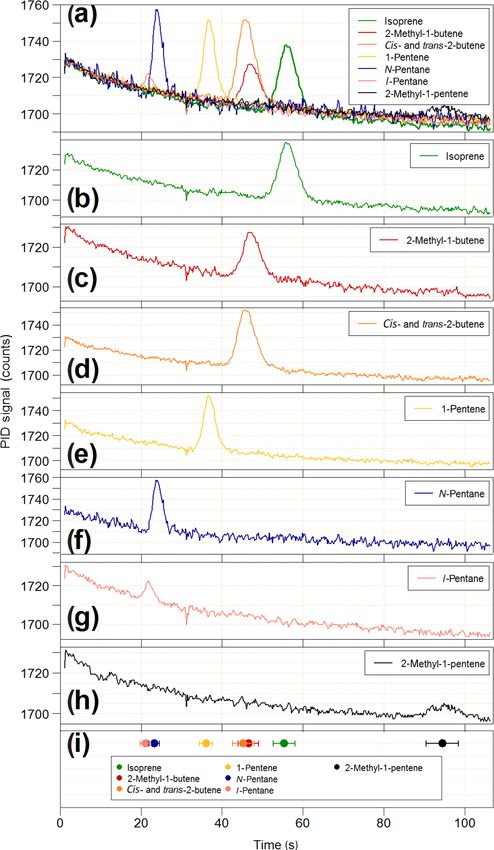
822                                                                                                      C. G. Bolas et al.: iDirac

meteorological variations, such as changes in incoming pho-            All of the limitations in the instruments currently used for
tosynthetically active radiation (PAR), temperature and at-         VOC detection drive the need for a field instrument that has
mospheric dynamics (Langford et al., 2010). High time reso-         the following six qualities:
lution data are required to capture trends in isoprene concen-
trations in real time. It is expected that isoprene emissions           1. lightweight, so that it is portable and can easily be car-
will be affected by global change (increasing temperatures,                ried and installed in environments difficult to access
land use change and increasing CO2 ) in the coming decades                 with traditional instrumentation;
(Bauwens et al., 2018; Hantson et al., 2017; Squire et al.,
2015). However, the overall magnitude and sign of changes               2. low-power, so that it is capable of running off-grid, al-
in isoprene emissions are still uncertain due to the many vari-            lowing measurements in locations with no mains power;
ables at play and the uncertainties in our emission models.
This, coupled with its large variability, makes it highly desir-        3. autonomous, so that it minimises operator involvement
able to improve the temporal and spatial coverage of isoprene              and maintenance;
measurements so that our understanding of its emissions via
                                                                        4. low gas use, so that it minimises the cylinder size re-
models can be validated against field data.
                                                                           quired and the number of site visits to replace gas cylin-
   Measurements of atmospheric hydrocarbons such as iso-
                                                                           ders;
prene are challenged by the difficulty in making measure-
ments in remote places. To date, in situ measurements of
                                                                        5. rugged and durable, so that it can withstand challenging
isoprene have been carried out using existing commercial
                                                                           environments; and
bench-top instruments, such as gas chromatographs (Jones
et al., 2011) and mass spectrometers (Noelscher et al., 2016;           6. relatively low-cost, so that many instruments can be de-
Yáñez-Serrano et al., 2015). These techniques differentiate                ployed at one time, maximising spatial coverage.
between VOCs either by separation (gas chromatography) or
by identification of their molecular ions based on mass-to-         Here we describe the development and validation of the
charge ratios (mass spectrometry). These instruments, while         iDirac, an instrument that fulfils the requirements listed
offering high precision and stability, are not built to withstand   above. It follows on from the philosophy of the µDirac
field conditions for long periods of time due to their need         (Gostlow et al., 2010), with portability, modularity, power
for power, temperature-controlled environments and special-         efficiency and autonomy at the centre of its design. The
ity carrier gases. This is especially true in under-sampled re-     iDirac also incorporates inexpensive microcontroller board
gions of high isoprene emissions, which are typically in re-        processors for advanced control and remote access to the in-
mote or challenging environments (e.g. tropical forests). In        strument. The core GC instrument and its operation are de-
these locations, instrument size, portability, autonomy, power      scribed in Sect. 2, while Sect. 3 presents the software used
demand and gas consumption severely limit the length of a           to control the instrument. Instrument performance is dis-
deployment. In addition, instrument cost and maintenance            cussed in Sect. 4, including calibration, accuracy, precision,
limit the number of instruments deployed at any one time,           sensitivity and separation ability. Finally, results from trial
and, hence, the spatial coverage of a field campaign.               runs in a controlled laboratory environment and deployments
   An alternative method to detect environmental VOCs is            in Malaysian Borneo and central England are presented in
with grab samples (Robinson et al., 2005). These can either         Sect. 5. Results on the impact of herbivory on canopy photo-
be whole air samples or adsorbent tubes, where air samples          synthesis and isoprene emissions in a UK woodland (Visako-
(or some specific air components) are collected in an inert         rpi et al., 2018) and on isoprene concentrations near the
vessel and analysed at a later date. While grab samples can be      Antarctic Peninsula (Nadzir et al., 2019) have already been
deployed in relatively large numbers, they typically provide        published.
low temporal resolution, making this approach unsuitable to
capture the rapidly changing concentrations of isoprene. In
addition, reactive compounds can degrade over time before           2    Practical description of the iDirac
analysis, and using this method for long periods, even with
some degree of automation, is very time and resource inten-         The iDirac is a portable gas chromatograph equipped with a
sive. Recent work showed that it is possible to retrieve iso-       photoionisation detector (GC-PID): the VOCs in an air sam-
prene abundances in the boundary layer using satellite mea-         ple are separated on chromatographic columns and then se-
surements by means of thermal infrared imaging (Fu et al.,          quentially detected by the PID. The instrument is built in-
2019). However, with uncertainties between 10 % and 50 %,           house and is lightweight, low-power and able to operate for
these retrievals would benefit from further validation from         up to several weeks or months autonomously. Its specifica-
ground-based instrumentation.                                       tions are shown in Table 1. Section 2.1 describes the basic
                                                                    outline of the instrument, and Sect. 2.2 describes the specific
                                                                    configuration of the instrument for isoprene.

Atmos. Meas. Tech., 13, 821–838, 2020                                                    www.atmos-meas-tech.net/13/821/2020/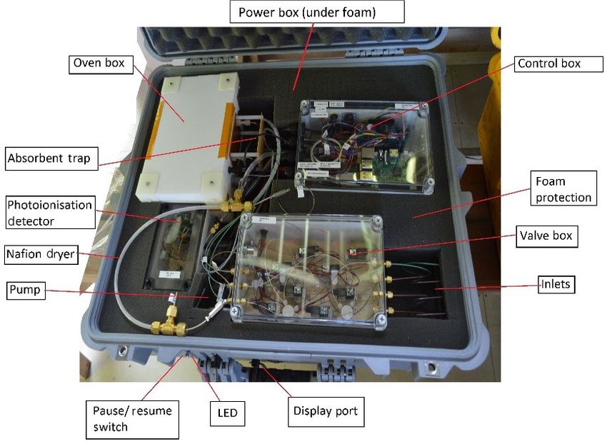
C. G. Bolas et al.: iDirac 823
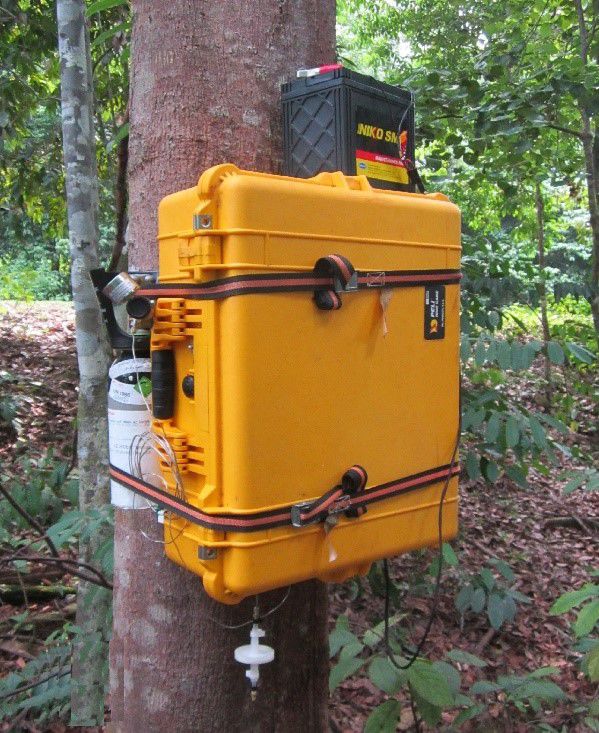
Figure 1. Interior of the iDirac showing the modular design of its component parts inside the main Peli case (22 cm × 61.6 cm × 49.3 cm)
Table 1. iDirac specifications. – a control box, containing microcontroller boards (Ar-
duino and Raspberry Pi), a number of electronic com-
Power 12 W ponents (e.g. solid state relays), the flowmeter and an
Weight 10 kg
SD card for data storage;
Voltage requirements 10–18 V – an oven box, containing the dual-column system, (pre-
Dimensions 22 cm × 61.6 cm × 49.3 cm and main columns), heating element and Valco valve;
Carrier gas High-purity nitrogen – a PID box, containing the photoionisation detector
(grade 5.0, or 99.999 %) (PID);
Calibration gas 10 nmol mol−1 (or ppb)
high-accuracy isoprene in nitrogen – a pump box, containing the pump and pressure differen-
tial sensor;
Limit of detection 38 pmol mol−1 (or ppt)
Precision 11 % – and a power box, containing power regulators and elec-
trical fuses.
On the exterior, the iDirac has a power socket and four
inlets for gas input. The inlets are for the nitrogen carrier
2.1 Core gas chromatograph physical design
gas, a calibration gas and two sample lines (samples 1 and 2)
between which the instrument can alternate.
The iDirac is built in a modular fashion, so that the vari- The general pneumatic design of the instrument is built
ous components are housed in six main plastic boxes (Pic- around two phases in the analysis cycle which are repre-
colo polycarbonate enclosures, IP67) packed in foam inside sented schematically in Fig. 2: a loading phase (load mode
a protective waterproof case (Peli 1600), as shown in Fig. 1. – pink), in which the analyte of interest is pre-concentrated
Details on the boxes and their contents are given below, and on an adsorbent trap, and an injection phase (inject mode
shown within the instrument in Fig. 1. The set-up is com- – purple), in which the analyte is desorbed from the trap
prised of the following: and directed into the oven for separation and, eventually, de-
tection. These two modes are controlled by a two-way 10-
– a valve box, containing eight solenoid valves to control port Valco valve (VIDV22-3110, mini diaphragm 10-port 2-
gas flow from the four inlets; position 1/1600 0.75 mm, Thames Valco) in the oven box,
www.atmos-meas-tech.net/13/821/2020/ Atmos. Meas. Tech., 13, 821–838, 2020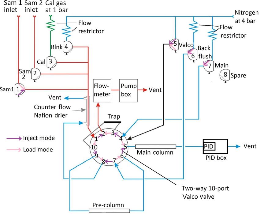
824                                                                                                               C. G. Bolas et al.: iDirac

Figure 2. Schematic representation of the iDirac operation. When in load mode (valve 5 off – pink), the contents of a gas source chosen
between valves 1, 2, 3 and 4 are pre-concentrated on the adsorbent trap. In inject mode (valve 5 on – purple), the VOCs in the trap are injected
into the dual-column system for separation and, eventually, detection. (“Sam” refers to sample, “Cal” refers to calibration and “Blnk” refers
to blank.)

which is activated by pneumatic actuation, by the set of                  and a main column, which performs the critical separation
solenoid valves in the valve box and by the pump.                         of the relevant analytes. The main column eluent is incident
   In load mode (Valco valve not activated, i.e. valve 5 off),            on the PID membrane, where the signal from the changing
one of four inlet gases (either Sample 1, Sample 2, the cal-              composition of the gas exiting the main column is detected.
ibration gas or the blank gas) is selected by switching on                   More details on the individual parts of this cycle are given
the appropriate solenoid valve (valves 1, 2, 3 or 4 respec-               below.
tively). By activating the pump, gas is drawn through the se-
lected inlet valve, dried in a Nafion counterflow system and              Inlet manifold and sample preparation
passed through an adsorbent trap where the analyte is pre-
concentrated. The sampled gas is vented into the Peli case                The inlet ports protrude from the side of the Peli case via
and then to the outside. A flowmeter is placed in series with             1/1600 bulkhead unions (Swagelok) and connect directly to
the sample flow and measures the gas flow through the trap.               the valve box, containing eight solenoid valves that act as gas
Once a pre-defined volume of gas has been sampled, the                    selectors. The Sample 1 (via valve 1), Sample 2 (via valve 2),
pump stops and the instrument enters inject mode. Labora-                 calibration gas (via valve 3) and blank nitrogen (via valve 4)
tory tests found no statistically significant difference in the           lines are all combined in a four-way SilcoNert-treated stain-
isoprene peak area between runs using the drier and runs by-              less steel Valco manifold (Z4M1, 1/1600 manifold, four in-
passing it.                                                               lets, Thames Restek). This manifold leads to the adsorbent
   In inject mode, the trap is flash-heated to 300 ± 5 ◦ C for            trap via a Nafion dryer (Nafion gas dryer 1200 , polypropy-
9 s to desorb the analyte from the adsorbent material. The                lene, Perma Pure MD-050-12P-2) which drives excess wa-
Valco valve is then pneumatically activated by switching                  ter vapour out of the gas flow by diffusion through a mem-
valve 5 on: the nitrogen carrier is flowed through the trap               brane with a counterflow of dry high-purity nitrogen. Valve
in the direction opposite to trap-loading, delivering the des-            5 is a direct line from the nitrogen inlet to the Valco valve
orbed compounds into the dual-column system where they                    for actuation, which requires a higher pressure (typically 4
undergo chromatographic separation. The oven consists of                  bar). Valves 6 and 7 control the nitrogen flow through the
a pre-column, which screens for large molecules (e.g. the                 columns: valve 7 activates the nitrogen flow through both
monoterpenes) whilst allowing smaller molecules through,                  columns in inject mode (when valve 5 is on), and through

Atmos. Meas. Tech., 13, 821–838, 2020                                                           www.atmos-meas-tech.net/13/821/2020/
C. G. Bolas et al.: iDirac                                                                                                    825

the main column only in load mode (when valve 5 is off).          is heated to 40 ◦ C using a heating element (PTC element
Valve 6 activates the nitrogen flow through the pre-column        enclosure heater, 15 W 12–24 V 40 C) which is fixed to the
for the back-flush in load mode. The nitrogen counterflow         baseplate of the oven using conductive paste. A fan mixes the
needed for the Nafion dryer is provided by valve 6 in inject      air inside the oven to ensure a uniform temperature through-
mode and by the pre-column back-flush vent in load mode.          out. The oven temperature exhibits diurnal variations (typi-
Gas lines downstream from valves 5, 6 and 7 leave the box         cally in the range of ±2 ◦ C) that appear to be driven by ambi-
via manifolds on the side of the box. Valve 8 is a spare valve    ent temperature. This introduces some variability in the iso-
with no current function.                                         prene retention time, but it is accounted for in the analysis of
   Flow restrictors upstream from valves 3, 4, 6 and 7 en-        chromatograms (see Sect. 3.3).
sure that the flow from the pressurised inlet lines does not         The sample is injected onto the pre-column (5 % RT-1200,
exceed the maximum flow through the flowmeter, and they           1.75 % BENTONE 34, SILPT-W, 100/120, 1.0 mm ID,
also reduce the gas demand of the instrument. The restrictor      1/1600 OD SILCO NOC, custom packed, Thames Restek, ∼
tubing used for the calibration line is red PEEK flow restric-    70 cm in length) via ports 9 and 10 on the Valco valve. Here,
tor (1/3200 OD, 0.00500 ID), and the one used for the nitrogen    isoprene and other small molecules travel faster through the
lines is black PEEK (1/3200 OD, 0.003500 ID). The rest of the     pre-column than bulky VOCs. After a set time (typically,
tubing is SilcoNert-treated stainless steel (Thames Restek,       30 s), once isoprene has passed through the pre-column, the
1/1600 OD, 0.0400 ID), which does not restrict the gas flow.      Valco valve is switched off, with valve 5 closing and valve 6
                                                                  opening, so that the pre-column is back-flushed. Thus, lighter
Sample adsorption/desorption system                               species, including isoprene, elute onto the main column,
                                                                  whereas larger molecules that are still in the pre-column
From the Nafion drier, the sample gas passes through ports        when valve 5 is switched off are removed from the column
1 and 10 of the Valco valve and into the adsorbent trap           system via the back-flush. This is important to avoid large,
when the instrument is in load mode. The trap consists of         less volatile species from entering the main column.
wide-bore stainless steel tubing (Hichrom, 1/1600 OD, 0.04600        The main chromatographic separation occurs on the
ID) containing one bed of adsorbent material between two          main column (OPN-RESL-C, 80/100, 1 mm ID, 1/1600 OD,
beds of glass beads, both crimped in place, with a coiled         SILCO NOC, custom packed, Thames Restek, ∼ 70 cm in
nichrome wire heating element surrounding the section of          length), based on the boiling point and polarity of the VOCs.
the tube corresponding to the adsorbent. The nichrome wire        This way, different species elute onto the detector at different
has a ceramic electrically insulating coating to prevent short-   times.
ing with the trap tubing. The adsorption of isoprene and
other VOCs takes place on a bed of approximately 10 mg
Graphsphere 2016 (formerly Carboxen 1016, Supelco, 60/80          Photoionisation detection system
mesh, 11021-U); Graphsphere 2016 is a carbon molecular
sieve that has been selected for its optimised recovery rate
of unsaturated short chain hydrocarbons upon thermal des-         The sample is directed from the outlet of the main column
orption. Different sorbent materials can be used for other        into a photoionisation detector (PID). The PID (Alphasense
species. The gas exiting the trap, now scrubbed of VOCs,          Ltd, PID-AH) operates by ionising any gas diffusing through
flows via ports 3 and 2 on the Valco valve into the flowmeter     a membrane covering a krypton lamp. Near-vacuum UV ra-
(Sensirion, ASF1430), which monitors the flow rate through        diation from the lamp ionises any molecule with an ionisa-
the trap. This is then integrated across the duration of sam-     tion potential of less than or equal to 10.6 eV. Isoprene, with
pling to calculate the total volume of gas sampled. When the      an ionisation potential of 8.85 eV (Bieri et al., 1977), is read-
desired volume (as specified by the user in the configuration     ily photolysed and, hence, detected by the PID with a sensi-
step – see Sect. 3) is reached, the valves from the sample        tivity of 140 % relative to that of isobutylene, which is used
inlet are closed and the pump is halted to stop the flow of       by the manufacturer as a reference compound in terms of PID
gas through the trap. The heating coil is flash-heated to des-    response. The ions generated by photoionisation produce a
orb the analyte from the adsorbent, while the Valco valve is      voltage change across an electrode system which is converted
switched to inject mode and valve 7 is activated, flushing the    to a digital signal by an analogue to digital converter (ADC;
desorbed VOCs onto the pre-column in the oven box with the        16 bit ADC four channel, Adafruit). The PID is turned on for
high-purity nitrogen carrier.                                     the duration of the elution from the dual-column system, and
                                                                  the data are collected at a frequency of 5 Hz. The chromatog-
Isothermal oven                                                   raphy run finishes once isoprene has eluted from the main
                                                                  column (typically 60–75 s after starting the back-flush). The
The flow containing the sample leaves the trap and enters the     data from the PID are then saved to a new file on an SD card
thermally insulated oven box. This enclosure, housed in insu-     by the Arduino Mega. A typical chromatogram showing an
lating material (lightweight display board, Kerbury Group),       isoprene peak is displayed in Fig. 3.

www.atmos-meas-tech.net/13/821/2020/                                                   Atmos. Meas. Tech., 13, 821–838, 2020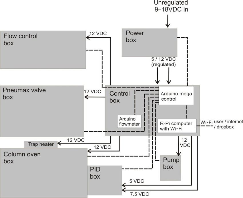
826                                                                                                        C. G. Bolas et al.: iDirac

                                                                        comparison with a primary gas standard. The calibration rou-
                                                                        tine is described in detail in Sect. 4.1.

                                                                        Power requirements for operation

                                                                        The instrument requires a power supply between 9 and 18 V.
                                                                        This can either be mains power or, alternatively, a battery.
                                                                        The incoming power is smoothed and regulated with two reg-
                                                                        ulators to stable 5 and 12 V outlets. The Arduino board mon-
                                                                        itors the supplied voltage in between runs in the case of the
                                                                        battery losing charge or power cuts. If the voltage drops, the
                                                                        iDirac switches to a power-save mode, where the oven, PID
                                                                        and valves are turned off to conserve power and the instru-
                                                                        ment waits for 20 min before again checking the input volt-
                                                                        age. Once a high enough voltage (typically 9 V) is detected,
                                                                        the various components are turned on again.
Figure 3. Typical chromatograms for (a) calibration, (c) sample and
(e) blank runs. The isoprene peak detected by the PID is around the     Flow control through the instrument
0.8 min mark. Panels (b), (d) and (f) show the combined baseline
and Gaussian fits to the observed data for each run type. Resid-        The flow through the instrument is driven by either upstream
uals are offset for clarity. All of the chromatograms are from the      pressure (in the case of the nitrogen and calibration gas
deployment in the Wytham Woods field campaign (see Sect. 5.3).          flows) or by the pump box (in the case of samples 1 and 2).
The calibration run is for 12 mL of a 11.6 ppb standard of isoprene     The pump box is an air-tight container with an inlet line and
in a nitrogen balance. The sample run is for a 150 mL ambient air       a vent. A diaphragm pump (DF-18, BOXER) withdraws air
sample (later quantified as 1.5 ppb isoprene). The blank run is for a   from the pump box and vents it outside, reducing the pressure
12 mL sample of grade 5.0 nitrogen.                                     inside the enclosure. The reduced pressure within the pump
                                                                        box causes air (from the Sample 1 and Sample 2 inlets) to
                                                                        be drawn through the system, via the trap and the flowme-
2.2   Instrument operation specifications                               ter. A pressure sensor (differential pressure sensor, Phidgets)
                                                                        monitors the pressure differential between the inside and the
Carrier gas and calibration gas                                         outside of the pump box. During a pump cycle, the pump
                                                                        is only activated when the pressure differential falls below a
Two gas cylinders are required to operate the iDirac: a pure            prespecified value (nominally 20 kPa). This method ensures
nitrogen supply and a calibration gas. Nitrogen is used as              a uniform flowrate and enables control over low flowrates
carrier gas through the dual-column system, as sample gas               (∼ 20 mL min−1 ), thus reducing the uncertainty in the vol-
for the blank runs and also to actuate the Valco valve. The             ume integration of the air sampled.
nitrogen supply is of at least grade 5 purity (correspond-
ing to ≥ 99.999 % nitrogen) to minimise interference from
impurities with the detection of isoprene. Typically, we use            3   iDirac software and hardware control and data
high-purity Nitrogen BIP (Air Products). The logistics of                   analysis
the measurement dictate the size of the nitrogen cylinder
used: for mobile deployments in the field, small portable               The iDirac is controlled using a dual Arduino system: an Ar-
cylinders (1.2 L) are ideal; whereas larger cylinders (10 L)            duino Micro board controls the gas flow components of the
are more suitable for long-term measurement, as they min-               instrument, whilst the main instrument control is achieved
imise the need for maintenance visits to replace the nitro-             with an Arduino Mega board. These two units communicate
gen cylinder. Typically, the iDirac can run continuously on a           with all of the sensors inside the instrument and read their
10 L nitrogen cylinder supplied at 200 bar for approximately            outputs. A Raspberry Pi computer acts as the interface be-
2 months. The calibration gas consists of a binary gas mix-             tween the user and the Arduino boards. A Python script is
ture of approximately 10 nmol mol−1 (or ppb) isoprene in a              run on the Raspberry Pi, allowing the user to configure the
nitrogen balance stored in a SilcoNert-treated 500 mL stain-            instrument with the desired parameters and read the sensor
less steel cylinder (Sulfinert sample cylinder, TPED, 1/400 ,           output from that of the Arduino. The Raspberry Pi desktop
Thames Restek). The use of cylinders with passivated inter-             can be accessed remotely via an ad hoc network, allowing
nal walls minimises the adsorption of isoprene on surfaces,             connection with a variety of interfaces. This control system
which would introduce biases in the measurement. The ac-                allows many of the parameters described above (e.g. sample
curate concentration of the calibration gas is determined by            volume and time spent in each column) to be changed.

Atmos. Meas. Tech., 13, 821–838, 2020                                                      www.atmos-meas-tech.net/13/821/2020/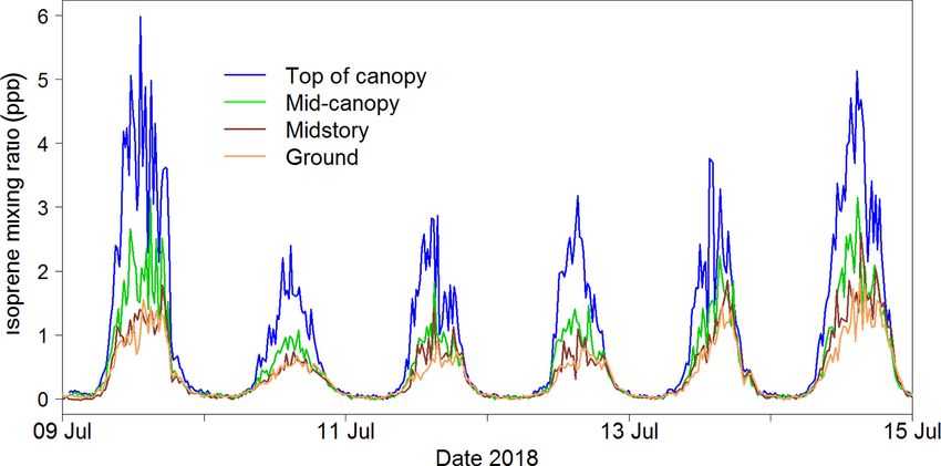
C. G. Bolas et al.: iDirac 827
Figure 4. Schematic of Arduino Mega connections.
3.1 Arduino control of internal electronics network, which can be connected to by laptops and mobile
phones in a fashion similar to a standard Wi-Fi network.
The instrument is controlled primarily using an Arduino Once connected to the network, a graphical desktop sharing
Mega 2560 board (Arduino Mega 2560, Arduino). This mi- system such as VNC viewer (VNC Viewer, RealVNC) allows
crocontroller has a number of analogue and digital ports and the user to navigate the Raspberry Pi desktop and manipulate
runs Arduino code (C and C++ commands) to control these the instrument.
ports. An SD breakout board is used (microSD card breakout Upon opening the Raspberry Pi desktop a purpose-written
board, Adafruit) to facilitate the use of an SD card to store Python script is launched automatically. A terminal win-
data in, while a real-time clock (RTC) board is used (real time dow is opened displaying the serial output from the Arduino
clock, ChronoDot ultra-precise, Adafruit) for time-keeping. Mega and transmitting data to the Arduino Mega via a se-
Figure 4 illustrates the various connections on the Arduino rial port connection. The latest version of this Python script
Mega. is freely available (https://github.com/cgb36/iDirac-scripts,
An Arduino Micro board (Arduino Micro, Arduino) last access: 5 January 2020). The Python script decodes in-
specifically reads the altimeter pressure sensor (located in the coming serial bytes from the Arduino Mega and displays
PID box) and the flowmeter, and sends these readings to the them in a user-friendly command line window. It is also pos-
Arduino Mega via a serial port. The use of the Arduino Mi- sible to restart and shutdown the instrument from the Rasp-
cro is justified as it simplifies the code on the Arduino Mega, berry Pi desktop. The Raspberry Pi requires a shutdown pro-
particularly as the flowmeter requires the use of a shifter to cedure, which can be done either physically with a switch on
convert the RS232 serial signal and several subsequent math- the side of the control box or from the virtual desktop envi-
ematical manipulations. The Arduino boards do not have a ronment.
shutdown procedure and can simply be unplugged.
3.3 Processing of chromatograms
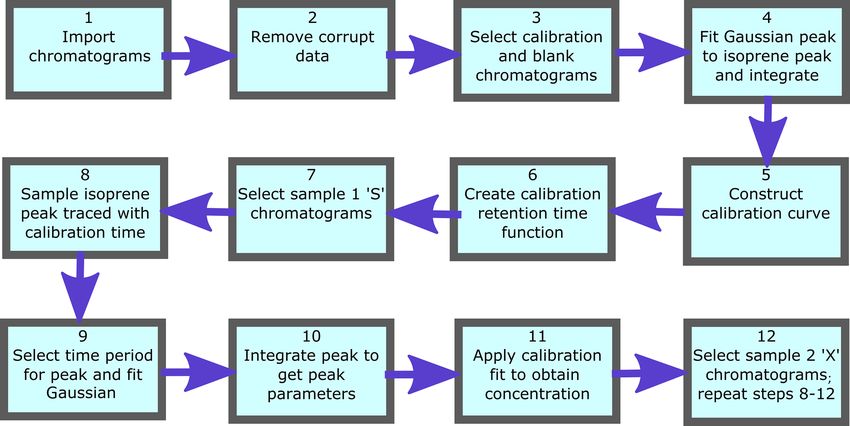
3.2 Description of Raspberry Pi user interface
To process numerous chromatograms in an automated fash-
The iDirac uses a Raspberry Pi (Raspberry Pi Model B V1.1, ion, a script was created that uses calibration runs to accu-
Raspberry Pi) as a user interface, allowing the instrument rately identify isoprene peaks in the sample runs and convert
to be controlled from a familiar desktop environment. The their integrated peak areas into mixing ratios. This script is
Raspberry Pi uses a Wi-Fi dongle to set up its own ad hoc written in Mathematica (v11.1.1). Figure 5 shows a flow dia-
www.atmos-meas-tech.net/13/821/2020/ Atmos. Meas. Tech., 13, 821–838, 2020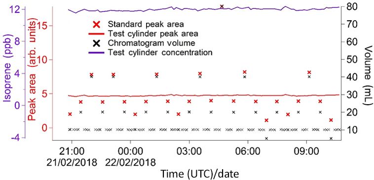
828                                                                                                   C. G. Bolas et al.: iDirac

gram for the main algorithms of the script. Firstly the data are   When there are insufficient calibration chromatograms to de-
read in, making sure that all the files are the correct size and   termine the isoprene peak retention time (e.g. less than four
do not contain any erroneous runs (e.g. corrupted or trun-         calibration runs in a day), it can be estimated using the col-
cated files) that may jeopardise the running of the script.        umn temperatures from the nearest calibration runs. If the
Each chromatogram file has an index field, either S, X, C or       spacing between calibration points is too great or the cali-
B which indicate if the chromatogram is a Sample 1, Sample         bration is carried out separately to the sampling, the interpo-
2, calibration or blank chromatogram respectively.                 lated calibration retention time values may not span the re-
    The calibration data are processed first. This involves se-    gion where the isoprene peak resides. In this case the column
lecting all calibration chromatograms (those with index “C”)       temperature and retention time of the most recent calibration
and plotting them for visual inspection. From the plot of          chromatograms are used to define a linear relationship. It is
all calibration chromatograms, the user specifies the regions      then possible to derive the isoprene retention time from the
that are used to fit to the isoprene peak and the baseline.        column temperature of the sample chromatogram.
A third-degree polynomial is fitted to the baseline over the
user-specified baseline intervals. A Gaussian curve is then
fitted to the baseline-subtracted chromatogram over the user-
specified peak interval. The peak height, width and position       4     Instrument performance
(equivalent to elution time) of the fitted Gaussian, as well
as the error in the fit (root-mean-square error, RMSE), are        4.1    Calibration of output chromatograms
logged. The elution time of the peak is retained in an in-
terpolated function over time. This function is then used to       The PID response to isoprene is calibrated using a pri-
locate the isoprene peak in the sample runs between two cal-       mary gas standard supplied by the National Physical Labo-
ibration runs. The blank runs (with index “B”) are included        ratory (NPL), certified as containing 5.01 ± 0.25 nmol mol−1
in this routine as they effectively represent calibrations with    (or ppb) isoprene in a nitrogen matrix (uncertainty provided
zero isoprene concentration. Subsequently, the peak area is        at the k = 2 level). The gas mixture is stored in a 10 L Ex-
plotted against the number of calibrant moles to obtain a re-      peris cylinder (Air Products); this type of cylinder has been
sponse curve. The number of calibrant moles, ncal , is defined     demonstrated to provide maximum stability (up to 2 years)
as                                                                 for VOC mixtures over time (Allen et al., 2018; Rhoderick
                                                                   et al., 2019). The primary standard is only used for cali-
ncal = (Vcal /Vmol ) · χcal ,                               (1)    bration in the laboratory; for field deployments, a smaller
where Vcal is the sampled volume of the standard during the        secondary gas standard is used instead. This is prepared
run, Vmol is the molar volume of an ideal gas and χcal is          manometrically by diluting a higher concentration parent
the isoprene amount fraction in the gas standard. A straight       mixture (100 nmol mol−1 isoprene in nitrogen, BOC) to ap-
line is then fitted to these data. Calibration procedures are      proximately 10 nmol mol−1 with high-purity nitrogen (BIP+,
described in depth in Sect. 4.1.                                   Air Products). This secondary gas standard is prepared in a
   The sample chromatograms are then selected as either            500 mL SilcoNert-treated stainless steel cylinder (Sulfinert
Sample 1 (runs with index “S”), or Sample 2 (runs with in-         sample cylinder, TPED, 1/400 , Thames Restek). This type of
dex “X”) and, as with the calibration runs, they are plotted       treated cylinder exhibits very good long-term stability for a
to visually inspect the data. Following this, we interpolate       number of VOCs (Allen et al., 2018; Rhoderick et al., 2019).
the retention times from adjacent calibration runs to the time     The exact isoprene amount fraction in the secondary stan-
of each sample runs, thus ensuring that the isoprene peak is       dard is determined by validating it against the NPL primary
identified correctly. This effectively takes variation in elu-     standard. This way, the measurements from the iDirac are
tion time caused by varying oven temperatures into account.        traceable to accurate primary standards. We routinely mea-
A baseline is fitted to the sample chromatograms in a simi-        sure the secondary standards against the primary standard
lar fashion to those fitted to the calibration chromatograms.      before and after field deployments to account for any degra-
Then a Gaussian function, constrained by certain boundaries        dation over time. However we have found no statistically sig-
(e.g. peak width within the average calibration peak width         nificant degradation over the time span of field deployments
±1 SD and retention time within ±4 s of the interpolated re-       (up to 5 months).
tention time), is fitted to the section of the chromatogram in-       Frequent calibration is needed not only to convert chro-
dicated by the interpolated calibration retention times. Using     matogram peaks into mixing ratios, but also to monitor
the sample peak area (Asam ), the sample volume (Vsam ), and       long-term trends in the detection system, including detector
the intercept (c) and gradient (m) of the calibration curve, the   drift and decreasing performance of the adsorbent trap. Any
isoprene mixing ratio in the sample, χsam , is calculated using    changes in isoprene elution time, which may be caused by
Eq. (2):                                                           changes in oven temperature, can affect the correct peak as-
                                                                   signment in chromatograms with multiple peaks. These ef-
χsam = (Asam − c)/m · (Vmol /Vsam ).                        (2)    fects can be easily addressed if frequent calibration chro-

Atmos. Meas. Tech., 13, 821–838, 2020                                                 www.atmos-meas-tech.net/13/821/2020/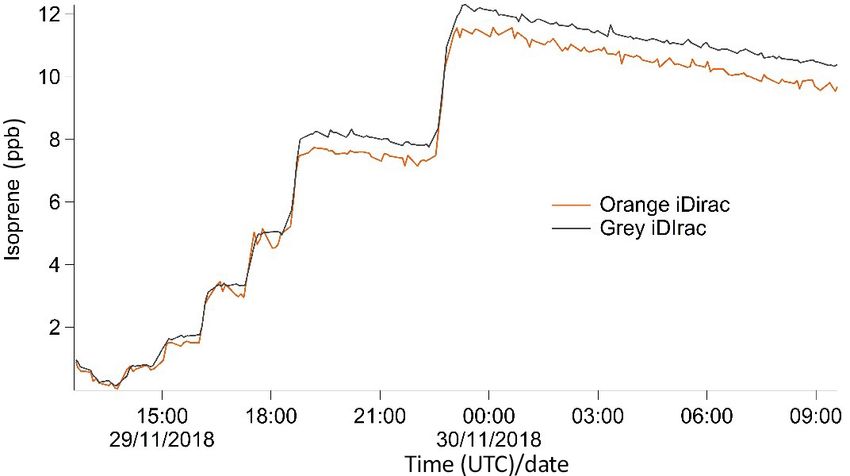
C. G. Bolas et al.: iDirac                                                                                                    829

Figure 5. Analysis script flow diagram.

matograms (which only have, by definition, one peak) are          obtained from the blank runs. A straight line is fitted to the
available.                                                        calibration data. A typical calibration plot is shown in Fig. 7.
   Calibration frequency is specified by the user in the in-      The straight line fit allows the determination of the fractional
strument set-up by selecting the number of samples to run         isoprene amount in the samples via Eq. (2) by extrapolation
between calibrations. For example, a calibration frequency        or interpolation, provided the sample volume and peak area
of “4” would correspond to a run of four sample chro-             are known. Typically, data are analysed in weekly segments,
matograms, followed by a calibration run. It is essential to      so that a calibration curve is obtained for each week.
perform a calibration run periodically to ensure that the posi-      The error in the sampled volumes is dominated by the
tion of the isoprene peak can be traced. Typically, a calibra-    dead volume in the gas lines before the trap (approximately
tion run is performed every 35 sample runs. As the mean           1.6 mL) combined with the uncertainty in the measurement
duration of a 150 mL sample run is approximately 9 min            of flow rates (1 %) and sampling times (0.05 %). The over-
(consisting of 7.5 min of sampling and 1.5 min of chromato-       all uncertainty in the volumes is estimated as 50 % for 3 mL,
graphic run), a calibration run is performed approximately        13 % for 12 mL, 3 % for 48 mL and 1 % for 200 mL.
every 5.25 h.                                                        As interpolation carries lower uncertainty than extrapola-
   The calibration cycle is programmed to be preceded and         tion, it is important to choose an appropriate value for the
followed by a blank run, in which the system samples from         user-specified calibration volume, so that the points in the
the high-purity nitrogen supply from valve 4. This allows any     calibration curve span the entire range of the sample runs
residual isoprene in the trap to be desorbed before and after     (as is the case in Fig. 6). Typically, 12 mL is suitable in an
calibration, and also allows the efficiency of desorption over    environment with relatively low (< 1 ppb) isoprene concen-
time to be monitored.                                             trations (e.g. remote oceans), whereas a higher value (20 mL)
   A calibration curve is obtained by varying the volume          is more appropriate when measuring in areas such as tropical
sampled in each calibration run. When configuring the in-         forests.
strument, the user specifies a calibration volume in millil-
itres, which is sampled every other calibration run. For the      4.2   Precision and accuracy of iDirac data
remaining calibration runs, the instrument is programmed to
sample a volume picked randomly from five possibilities: the      Precision
user-specified calibration volume, the user-specified calibra-
tion volume multiplied by 2 or 4, and the user-specified cal-     The precision of the instrument was determined as the rela-
ibration volume divided by 2 or 4. For instance, for a run        tive standard deviation in isoprene peak area from calibration
configured with a calibration volume of 12 mL, half the cali-     chromatograms with the same user-specified volume (typ-
bration runs would be of 12 mL samples and half would be a        ically, more than 50 % of the total calibration runs in any
random mixture of 3, 6, 12, 24 and 48 mL samples. A typical       given measurement sequence, as detailed in Sect. 4.1) and
time sequence of isoprene peak areas from different calibra-      from the same calibration cylinder. For instance, in the cal-
tion volumes is shown in Fig. 6. A calibration curve is then      ibration sequence shown in Fig. 7, this corresponds to the
obtained by plotting these peak areas against the number of       runs of 12 mL samples. Following analysis of the scatter of
calibrant moles (as defined in Eq. 1). The zero moles point is    these data points, the instrument precision is determined to
                                                                  be ±10.4 % in the field (compared with < 5 % in the labo-

www.atmos-meas-tech.net/13/821/2020/                                                  Atmos. Meas. Tech., 13, 821–838, 2020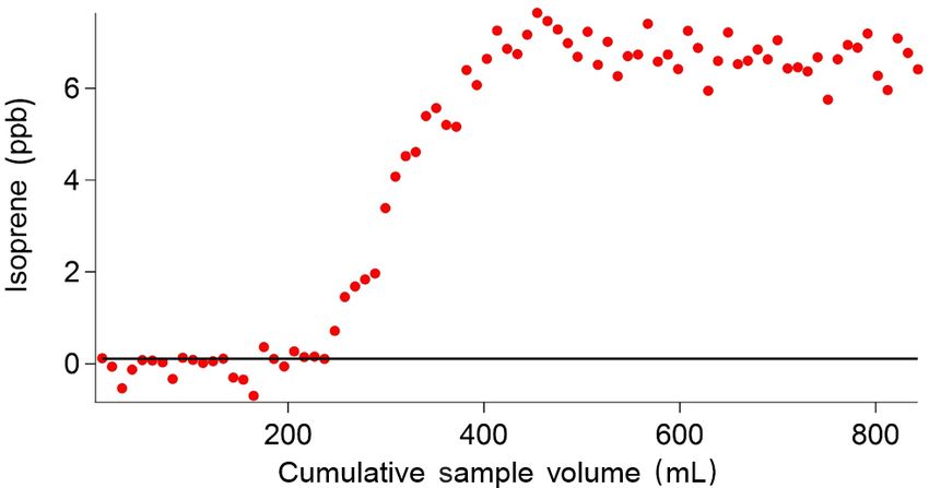
830                                                                                                            C. G. Bolas et al.: iDirac

Figure 6. Typical sequence of isoprene peak areas for runs with varying calibration volumes. These, once split into weekly segments, are
used to produce a calibration curve (see Fig. 7). The calibration runs with the standard user-specified sampled volume (red data points) are
used to calculate the instrument precision on a weekly basis (see Sect. 4.2). Peak areas from sample runs (grey data points) are also shown
to illustrate how the calibration peak areas span the entire range of sample values, minimising the need for extrapolation. This plot was
produced using data from the Wytham Woods field campaign (see Sect. 5.2).

                                                                        Accuracy

                                                                        One of the main components of the accuracy of the instru-
                                                                        ment is the uncertainty in the isoprene amount fraction in
                                                                        the NPL standard, and how this is propagated to the isoprene
                                                                        amount fraction in the secondary gas standard used in the
                                                                        field. Therefore, it is essential that the concentration of the
                                                                        secondary calibration cylinder is determined as accurately as
                                                                        possible by comparing it to the NPL primary standard. This
                                                                        is carried out in the laboratory, typically before and after each
                                                                        field deployment.
                                                                            An example of this concentration determination is shown
                                                                        in Fig. 8. XLGENLINE, a freely available generalised least-
                                                                        squares (GLS) software package for low-degree polynomial
                                                                        fitting (Smith, 2010), is used to estimate the uncertainty in the
Figure 7. Calibration plot for isoprene for the week of 2–              isoprene amount fraction in the secondary calibration cylin-
8 July 2018 from the Wytham Woods field campaign. Error bars in         der. This is carried out in two steps. First the calibration data
the area correspond to the precision of the measurement (±10.4 %).      (i.e. the peak areas and sampled volumes from the NPL pri-
Error bars in the calibrant moles are estimated from the uncertain-     mary standard) are run through XLGENLINE to produce a
ties in the secondary standard used and in the volume of gas sam-       calibration line with an associated uncertainty envelope. In
pled.                                                                   the second step, this calibration curve is used to convert the
                                                                        peak areas from the secondary standard (i.e. the “unknown”)
                                                                        into concentrations and their associated uncertainties. For
ratory). This procedure is carried out for each weekly seg-             secondary calibration cylinders, this is estimated as ∼ 3.5 %
ment of the data so that the measurement precision can be               (±1SD). A similar procedure is applied to field data to esti-
routinely monitored over time which is especially useful for            mate the uncertainty in the ambient isoprene concentrations
long deployments.                                                       (now using the secondary standard for the calibration). This
                                                                        is estimated as ∼ 10 %–12.5 % (±1SD).
                                                                            Co-elution of interfering species can also affect accuracy.
                                                                        Tests targeting specific potential interferents are described in
                                                                        Sect. 5.1 and show that these species do not overlap with
                                                                        the isoprene peak in the chromatograms. However co-elution

Atmos. Meas. Tech., 13, 821–838, 2020                                                        www.atmos-meas-tech.net/13/821/2020/
C. G. Bolas et al.: iDirac 831
Figure 8. Summary plot of a concentration determination experi-
ment. The primary reference gas mixture is used as the standard
in the calibration runs, and the secondary gas mixture under test is Figure 9. Time series plot showing isoprene mixing ratios from the
used as the sample. grey and orange iDirac instruments.
with unknown (or not tested for) species, albeit unlikely, can as the standard deviation in the PID signal in a section of the
never be fully ruled out. If these species have longer life- blank chromatogram corresponding to the isoprene elution
times than isoprene, the observed night-time abundances at- time. The instrument response factor is calculated from the
tributed to isoprene can be used as the upper limit of poten- isoprene peak height in the calibration runs and the isoprene
tial interference of unknown co-eluters (assuming they are amount fraction in the standard. This allows the calculation
trapped with the same efficiency and have the same PID re- of the minimum concentration needed to give rise to a signal
sponse as isoprene). The isoprene night-time mixing ratio is that would return a S/N of 3. This is identified as the limit
50 ppt for the data shown in both Figs. 14 and 15. There- of detection and is monitored routinely during field deploy-
fore, we estimate the instrument accuracy for field data as ments and laboratory tests. The limit of detection for two ver-
the combination of the propagated uncertainty from the stan- sions of the iDirac, the grey and the orange instruments (see
dard (10 %–12.5 %) and the potential co-elution of long-lived Sect. 5.1 for details), during their deployment in the Wytham
species (50 ppt). This correspond to an overall accuracy of Woods field campaign (See Sect. 5.2) were 108 and 38.1 ppt
±1.2 ppb for a 10 ppb isoprene sample, ±0.13 ppb for a 1 ppb respectively. These are higher than the limit of detection de-
isoprene sample and ±51 ppt for a 100 ppt isoprene sample. termined in the laboratory (46 and 19 ppt respectively). The
Deviations of peak shape from a simple Gaussian function difference between field and laboratory sensitivity is due to
also impact accuracy by introducing a bias in the reported greater noise in the field measurements, as a result of less
peak areas. However this is limited to high volume, high con- controlled environmental conditions. The difference in the
centration samples and can add ∼ 2 % to the overall accuracy limit of detection between the two instruments is attributed
budget. to differences in instrumental noise (the noise in the orange
iDirac is 10 %–20 % greater than that from the grey iDirac),
4.3 Sensitivity of the iDirac to isoprene different responses of the PIDs to isoprene, and using traps
at different stages of their life cycle (refer to Sect. 5.3.2 and
The instrument’s sensitivity can be adjusted by changing the Fig. 16).
volume of the sample being analysed. For high concentra-
tions (e.g. strong leaf emissions) a smaller volume should
be used to avoid nonideal behaviour of the adsorbent, as de- 5 Tests in the laboratory and field deployments
scribed by Peters and Bakkeren (1994). The instrument has
The iDirac has been tested in a series of laboratory evalua-
an effective upper volume limit of 250 mL (see Sect. 5.1) and
tions, during a deployment at a field station in a tropical for-
a lower limit of 3 mL. The volume integration becomes unre-
est in Sabah, Malaysia, and in a research forest in Wytham
liable below 3 mL due to the additional uncertainty brought
Woods, UK.
about by the dead volume before the trap (approximately
1.6 mL). Conversely, when ambient levels of isoprene are 5.1 Laboratory tests
low (< 500 ppt), large sample volumes (200 mL) should be
used. Sample volumes lower than or equal to 200 mL are Intercomparison of two versions of the iDirac
used in order not to exceed the trap breakthrough volume
(see Sect. 5.1). Two iDirac instruments (orange and grey) were compared
The limit of detection is determined for a specific set of against one another, with the two instruments sampling from
runs by allowing a signal-to-noise ratio (S/N) of 3. The a chamber containing a controlled isoprene concentration
blank runs are used to calculate the noise, which is defined that was varied over time. The orange and grey iDirac in-
www.atmos-meas-tech.net/13/821/2020/ Atmos. Meas. Tech., 13, 821–838, 2020832 C. G. Bolas et al.: iDirac
Figure 11. Results of the breakthrough volume tests. Each data
point is an individual sample run of 10 mL. A solid black line in-
dicates a threshold (set at a LOD of 0.108 ppb), above which the
breakthrough volume is exceeded.
Figure 10. Scatter plot with the 1 : 1 line showing the 15 min aver-
age values for the grey and orange iDirac instruments.
Breakthrough tests
The breakthrough volume for the adsorbent traps used in the
struments both had inlets inside the chamber with identi-
iDirac was determined. This is a test that evaluates the vol-
cal filters (polyethersulfone, 0.45 µm pore-size) and the same
ume of gas that causes isoprene to pass through the trap in
1.5 m length of PTFE 1/1600 tubing, and they were placed as
a single sample run, and is typically independent of the an-
close to one another as possible. The gas within the cham-
alyte concentration (Peters and Bakkeren, 1994). This test
ber was well mixed by two large fans. Gas from a 700 ppb
is performed by placing an additional adsorbent trap in the
isoprene (±5 %) in a nitrogen balance mixture (BOC) was
instrument upstream of the main trap, at the exit of valves
flow-controlled into the chamber at 80 mL min−1 for differ-
1–4 from the valve box. Each run sampled 10 mL of a mix-
ent time periods to change the concentration. The chamber
ture of 5 ppb isoprene and 5 ppb α-pinene in a nitrogen bal-
was not flushed, and the only exchange out of the chamber
ance. When the breakthrough volume of the additional trap
was slight seepage through several small holes around the in-
is exceeded, isoprene effectively ‘breaks through’ from the
lets. The concentration was varied stepwise from 0 to 12 ppb.
additional trap onto the main trap, so that it is injected onto
The instruments were calibrated using the same calibration
the dual-column system and a peak is observed in the chro-
standard (8.3±0.6 ppb isoprene in nitrogen), which was con-
matograms. The sum of all the volumes of the runs in which
nected to both instruments via a tee-piece.
isoprene was not observed (i.e. pre-breakthrough) gives the
The results from this experiment are shown in Fig. 9.
breakthrough volume. This value effectively acts as an upper
The orange iDirac under-reads by 6.6 % relative to the grey
limit of the volume of gas that the instrument can sample.
iDirac, and this is particularly evident at high concentrations
Figure 11 shows a typical example of such test, in which a
(> 8 ppb). Figure 10 shows these data as a scatter plot of the
breakthrough volume of 250 mL was determined. Thus, the
15 min average values from either instrument, and, again, it
instrument is set to sample volumes up to 200 mL so that the
can be seen that the orange iDirac under-reads slightly. This
breakthrough volume is never exceeded.
under-reading is partly attributed to the systematic underes-
timation of the peak areas from the orange runs due to peak Co-elution of interfering species
tailing. Integration of a subset of chromatograms using an ex-
ponentially modified Gaussian function showed that a simple The PID used in the iDirac is sensitive to all molecules with
Gaussian fit underestimates peak areas from the orange in- ionisation energies less than or equal to 10.6 eV, which in-
strument by up to 2 %. No significant degree of tailing was cludes the vast majority of biogenic and anthropogenic VOCs
observed in the runs from the grey instrument. Despite this with the exclusion of ethane, acetylene, propane, methanol,
slight discrepancy between the output isoprene concentration formaldehyde and a number of halogenated hydrocarbons.
from the two instruments, it should be noted that the two Therefore, it is possible that species co-eluting at the same
iDirac instruments perform within their specified accuracies time as isoprene might be detected and erroneously identified
(see Sect. 4.2). as isoprene, thus leading to reporting of spurious concentra-
tions. The stationary phase in the main column is selected to
achieve good separation of isoprene from VOCs of similar
polarity and boiling point. This is tested in a series of co-
elution experiments, in which the elution time of a number of
potentially interfering species was determined and their sep-
Atmos. Meas. Tech., 13, 821–838, 2020 www.atmos-meas-tech.net/13/821/2020/C. G. Bolas et al.: iDirac 833 Figure 12. Results of the co-elution tests on the iDirac. (a) Overlaid chromatograms of isoprene (green line) and six potential interfering species: 2-methyl-1-butene (red line), cis- and trans-2-butene (orange line), 1-pentene (yellow line), n-pentane (blue line), i-pentane (pink line) and 2-methyl-1-pentene (black line). The chromatograms of each individual species are shown in panels (b–h). The co-elution tests are summarised in panel (h), where the elution time of each species (filled circles) is plotted along with its peak width (FWHM) to assess peak separation. www.atmos-meas-tech.net/13/821/2020/ Atmos. Meas. Tech., 13, 821–838, 2020
834                                                                                                  C. G. Bolas et al.: iDirac

                                                                Figure 14. Time series for isoprene at a secondary forest site in
                                                                Sabah (Malaysian Borneo) in 2015.

                                                                a wider range of compounds, including oxygenated products
                                                                from the oxidation of isoprene.
                                                                   Co-elution and multiple peaks appearing in a chro-
                                                                matogram are also addressed in the Mathematica script de-
                                                                scribed in Sect. 3.3. To ensure that the isoprene peak is cor-
                                                                rectly assigned, the script looks for a peak in a relatively nar-
                                                                row region of the chromatogram, which is based on an in-
                                                                terpolation of the elution time from the two nearest calibra-
                                                                tion runs. This algorithm has relatively low tolerance, so that
                                                                peaks that are more than 4 s away from the predicted isoprene
                                                                elution time are not considered.
Figure 13. iDirac deployed in a tropical forest environment.       We observe a consistent discrepancy in the isoprene elu-
                                                                tion time between the calibration and sample runs. The elu-
                                                                tion time of isoprene is typically 1.7 s greater in a sample
aration from isoprene assessed. The VOCs under test were        run than in a calibration run. This is an artefact of the trap
chosen based on the column specifications reported by the       adsorption process and the resulting tailing of the peak. For
manufacturer, which identified i- and n-pentane, 1-pentene,     large volumes and low concentrations (e.g. a 150 mL field
cis- and trans-2-butene, 2-methyl-1-butene and 2-methyl-1-      sample at 0.5 ppb), the isoprene band in the adsorbent trap is
pentene as potentially co-eluting with isoprene. Gas samples    very broad and resides in the trap for a longer time, so it tails
containing 10–20 ppb of each interfering VOC are prepared       very strongly. For a high-concentration low-volume sample
in 3 L Tedlar bags by two-step dilutions from the “pure”        (e.g. a 12 mL calibration run at 10 ppb), the isoprene band
substance (Sigma Aldrich, purity typically > 98 %) using        in the trap adsorbent is very sharp, it desorbs quickly and,
grade 5.0 nitrogen (purity > 99.999 %). For each interfer-      hence, it tails less. This difference in elution times is much
ing species, the iDirac alternated between sampling from one    smaller than the distance to the nearest interfering species
of the Tedlar bags and sampling from a gas cylinder con-        (2-methyl-1-pentene, which elutes ∼ 7 s before isoprene).
taining only isoprene in nitrogen. The results of these mea-       The peak width and the RMSE from the Gaussian fit, re-
surements are summarised in Fig. 12. Figure 12a illustrates     trieved from the fitting routine described in Sect. 3.3, can
overlaid chromatograms for each species, and the individual     also be used to evaluate the presence of co-eluting species.
chromatograms are shown in Fig. 12b–h. Figure 12i sum-          An additional peak overlapping to some degree with the tar-
marises the different elution times taking the width of each    get isoprene peak in a sample run would cause a change in
peak (full-width at half maximum – FWHM) into account to        the peak shape. This would result in values for the fitted peak
better assess separation. The isoprene peak is well separated   width and RMSE that are different from those from the cal-
from all interfering VOCs, whereas we observe poor sepa-        ibration runs. For this reason, we use the width and RMSE
ration between cis- and trans-2-butene (which are not sepa-     from the calibration runs to define a range of acceptable peak
rated at all and appear as a single peak in Fig. 12d) and 2-    widths and RMSE values (equal to the mean value ±1SD).
methyl-1-butene, as well as between i- and n-pentane. Sim-      Any peaks from sample runs exceeding this range are flagged
ilar tests were carried out for acetone and ethanol, and we     for further analysis.
found that they eluted outside of the chromatographic win-
dow considered here. These results lend confidence to the
unequivocal assignment of the isoprene peak in each chro-
matogram. Work is ongoing to determine the elution time of

Atmos. Meas. Tech., 13, 821–838, 2020                                               www.atmos-meas-tech.net/13/821/2020/
C. G. Bolas et al.: iDirac 835
ibration routine) and several issues with instrument function
(e.g. warm-up time) that have been addressed in subsequent
versions.
5.3 Deployment of the iDirac during the Wytham
Woods field campaign (University of Oxford)
5.3.1 Experiment description
The instrument was deployed in Wytham Woods (Oxford-
shire, UK), a temperate mixed deciduous forest owned and
Figure 15. Portion of the isoprene mixing ratio time series mea- managed by the University of Oxford. A large fraction of
sured during the Wytham Woods field campaign (UK) at four trees at this site are pedunculate oaks (Quercus robur), which
heights within a forest canopy in the summer of 2018. are known strong isoprene emitters (Lehning et al., 1999).
One iDirac was deployed on the canopy walkway facility, a
platform ∼ 15 m above ground resting on a scaffolding sup-
Long-term tests port that allowed access to crown-level measurements, while
another iDirac was installed at ground level. As each instru-
The performance of the instrument in the field for long pe- ment has two inlets, this allowed sampling at four heights
riods of time has been assessed during several deployments. across the canopy with a view to investigating the isoprene
These are described in detail in Sect. 5.2 concentration gradient within the canopy. Both iDirac instru-
ments were run off-grid, powered only by solar-powered bat-
5.2 Deployment of the iDirac in Sabah, 2015 teries. The experiment and results are described in detail by
Ferracci et al. (2020a) and Otu-Larbi et al. (2019). Data were
Following laboratory development and testing, the iDirac had collected from May to October 2018; here, the performance
its first field deployment at the Bukit Atur Global Atmo- of the instruments is assessed for more than 5 months of con-
sphere Watch (GAW) station in the Danum Valley Conserva- tinuous use in a forest environment.
tion Area in Sabah (Malaysian Borneo) as part of the “Biodi-
versity and land-use impacts on tropical ecosystem function” 5.3.2 Results and discussion
(BALI) plant traits campaign. This campaign ran from May
to December 2015. The instrument was principally used to The iDirac captured isoprene concentrations from 25 May
carry out individual leaf measurements in the field. The re- to 29 October 2018. Gaps in the data were generally due to
sults from the individual leaf measurements are being written power issues arising from insufficient solar charging of the
up for publication elsewhere. batteries. A section of the isoprene time series is shown in
The other type of measurements taken in Sabah during this Fig. 15. The diurnal pattern of isoprene is clearly visible, and
timeframe were longer duration runs, in which the instrument the vertical concentration gradient is also apparent.
took autonomous measurements of ambient air at the field The iDirac proved capable of measuring isoprene abun-
site continuously. These measurements consisted of attach- dances continuously through the day, spanning from concen-
ing the iDirac to a tree at a height of approximately 1 m, with trations as high as 8 ppb in the height of the summer to effec-
a battery and a 1.2 L N2 cylinder attached to it, and running tively zero at night-time.
repeat samples until either the battery ran flat or the gas sup- The lifetime of the absorbent trap can be assessed by
ply was exhausted. The aim of these measurements was to examining the calibration curves over time. The dataset is
obtain an isoprene diurnal profile and observe how this var- analysed in weekly segments, with a calibration curve con-
ied with different types of forest. These tests also allowed us structed for each week. This allows for the calibrated data to
to test the feasibility of leaving the instrument running for account for any drift in sensitivity. The calibration plots ex-
long periods of time. A picture of the iDirac measuring am- hibit a clear drift as time progresses, as shown in Fig. 16, with
bient air in the rainforest in Borneo is shown in Fig. 13. calibration chromatograms later in the time series showing a
The ambient air measurements demonstrated that the in- lower peak area for the same concentration. Once the trap is
strument could easily measure the changes in isoprene con- replaced, higher sensitivity is recovered (shown as the green
centration in the ambient air and that the inlet drying sys- dashed line in Fig. 16a and the green square in Fig. 16b).
tem could cope with the high humidity of the rainforest. An This drift is attributed to the gradual degradation of the
example from a secondary forest site is shown in Fig. 14. trap as a result of repeated absorption/desorption cycles, with
This was the first deployment for the iDirac, and it proved to exposure to high concentrations of VOCs and oxygen. As
be a success with respect to taking reliable measurements. It each week of data represents approximately 1000 absorp-
also highlighted areas for instrument development (e.g. cal- tion/desorption cycles, it is likely that the absorbent in the
www.atmos-meas-tech.net/13/821/2020/ Atmos. Meas. Tech., 13, 821–838, 2020You can also read