Impact of node count on energy-optimal control of stratified vertical water heaters in smart grid applications
←
→
Page content transcription
If your browser does not render page correctly, please read the page content below
Impact of node count on energy-optimal control of stratified vertical water
                    heaters in smart grid applications

                                 M. Ritchie a , J.A.A. Engelbrecht a , M.J. Booysen       a,∗

                          a Department   of E&E Engineering, Stellenbosch University, South Africa

Abstract
   The energy requirements for an Electric Water Heater (EWH) accounts for 40% of a household’s total
energy consumption and 30 % of greenhouse gases emissions. The flexibility of the device to store thermal
energy for long periods highlights how the intensity of the grid demand can be alleviated by implementing
demand-side management (DSM) strategies. In this paper, we evaluate energy savings that can be achieved
by modelling the EWH as a variable number of multiple nodes and providing it with optimal control with
perfect foreknowledge of the hot water usage profile. We simulated 77 household’s for all four seasons and
determined that an average daily energy saving of 6.24% for temperature-matching and 16.3% for energy-
matching can be achieved for a 20-node EWH. We also evaluated how increasing the number of nodes of the
EWH when determining the optimal planning affects energy savings. It was concluded that using more than
four nodes produced diminishing returns.
Keywords: Smart grid; optimal control; electric water heaters

1. Introduction
    Demand-side management (DSM) focuses on reducing the demand on the energy grid by implementing
strategies that shift energy consumption during peak to off-peak hours or by decreasing the overall energy
usage. The EWH accounts for as much 40 % of a household’s total energy consumption and 30 % of its green-
house gases emissions (Skinner et al., 2012; Nejat et al., 2015; Hohne et al., 2019; Mabina et al., 2021). This
makes the thermal storage device convenient for reducing a household’s energy demand because it provides
the flexibility of storing energy for long periods with small energy losses (Ericson, 2009). The implementation
of advanced control strategies can greatly improve the energy efficiency of EWHs by minimising energy loss,
enhancing user comfort, and preventing the risk of Legionella (Pomianowski et al., 2020). Legionella pneu-
mophila is a bacteria that is potentially harmful to humans and grows inside water tanks if the temperature
remains low for long periods. The bacteria can be sterilised if the tank is sufficiently heated at least once a
day (Armstrong et al., 2014; Stone et al., 2019; Stout et al., 1986).
    Taking South Africa as an example, the country has suffered from loadshedding, a term that refers to
scheduled regional power interruptions, because of the incapability of the electricity supply to meet the
country’s growing demand, and is expected to continue for another five years (ESKOM, 2021; Jamie McKane,
2021). Since the country’s primary energy source is coal, contributing to approximately 88 % of the electricity
generation, reducing the overall energy demand can lessen the impact of carbon emissions (Mathu, 2017).
    Determining the effective energy savings of control strategies requires accurate modelling of tanked water
heaters and is significantly influenced by the accuracy of the hot water usage data (Dongellini et al., 2015;
Spur et al., 2006). Fernández-Seara et al. (2007) performed an experimental analysis of a vertically-orientated
EWH with 11 temperature sensors to determine the thermal behaviour during static operation. The results
indicated that stratification occurs inside the tank due to varying water temperature at each layer and the
temperature differences were most significant at the lower parts of the tank.
    Most related studies have been found to utilise one of the following four EWH models: A one-node
model assumes that the temperature of the tank is at a uniform temperature. A two-mass composite model

  ∗ Corresponding author
    Email address: mjbooysen@sun.ac.za ()

Preprint submitted to Elsevier                                                                       July 19, 2021
Nomenclature
∆t Sampling period Thys Hysteresis
c Specific heat capacity of water Tinlet Inlet water temperature
Etank Thermal energy of EWH TLegionella Legionella prevention temperature
Etank,n Thermal energy of node n Tmax Maximum EWH temperature
J Cost function Tmin Minimum EWH temperature
ρ Density of water Toutlet Outlet water temperature
Pelec Power supplied by heating element Tset Set-point temperature
Prated Rated power of heating element Tstart Initial temperature boundary condition
Qdraw Outlet volumetric flow rate Ttank Water temperature of EWH
RT Thermal resistance of EWH Ttank, n Water temperature of node n
RTH Thermal resistance of thermocline Vtank Tank volume of EWH
tf Final time instant Vtank,n Tank volume of node n
ti Initial time instant Tusage Minimum usage temperature
Tamb Ambient temperature u Control input
Tend Final temperature boundary condition x System state vector
represents the body of water inside the tank as an upper and lower layer. The upper node is either at a higher
or equal temperature to the lower node and water stratification in the layers is not accounted for. A two-node
model, similar to the previous model, does not neglect the transfer of heat that occurs at the thermocline of
the two bodies of water. The volume of each node also varies: hot water drawing depletes the volume of the
upper node and cold water entering the tank is mixed with the lower node. The multi-node model models
the tank as a finite number of nodes stacked on top of each other. Each node has a constant volume and
distinct temperature and stratification occurs at the boundary of adjacent nodes. More information on these
models can be found in (Kepplinger et al., 2019).
This paper determines the energy savings achieved by optimal control of an EWH with perfect foreknowl-
edge of the hot water usage profile, by evaluating the impact of the number of nodes by which the natural
stratificatio is modelled. The EWH simulator and optimisation algorithm were developed in Jupyter Notebook
and using the Python programming language. The paper is structured as follows: Section II reviews work
related to the optimal control of EWHs. Section III describes the hot water data and simulation setup for
obtaining the results. Section IV presents the development of the multi-node EWH model and optimisation
algorithm. Section V and VI show the results and conclusion of this study.
1.1. Contributions
A control strategy is developed for the EWH optimal control problem which is formulated to determine
the optimal switching schedule of the heating element to minimise the electrical energy usage while satisfying
the comfort of the user. The novelty of the developed optimisation algorithm is contributed by its capability
to model an EWH with N nodes in the optimal planning. The novel results produced in this study determines
the theoretical optimal energy savings that are achieved by a multi-node EWH with perfect foreknowledge
of the hot water usage profile. This study also determines the maximum number of EWH nodes required for
optimal planning before the results show diminishing returns.
2. Related Work
Gholizadeh and Aravinthan (2016) evaluated the cost benefits of managing the set-point temperature and
heating scheduling of residential EWH’s. They reported that the savings were 5.9 % to 6.4 %. However, their
study used random variations of the ASHRAE standard to represent typical water profiles instead of using
real data. The shortcoming of using this water usage model is that the hot water profiles are generalised and
predicted.
Booysen and Cloete (2016) determined energy savings using a two-node EWH model developed by Nel
et al. (2016). Their aim was to understand the energy impact of non-optimal manual schedule control on
EWH’s and they performed field trials of four water heaters and a controlled laboratory experiment of a single
2water heater to validate their results. They confirmed that the simulated results accurately described the
measured results. They obtained energy savings of 29 % but did not consider temperature or energy-matching
the EWH to a baseline scenario during water usages.
Booysen et al. (2019a) determine how much energy can theoretically be saved by providing the optimal
control of an EWH for known water usage profiles, using only a single node to model the water as a lumped
mass. Their study used hot water draw data that was measured over 20 days for 30 EWH’s installed in South
African household’s. They used dynamic programming to determine the optimal heating schedule for the
heating element to achieve the best savings. They performed simulations for cases where the temperature
and energy are matched to the baseline condition during water usages, and the average energy savings were
8 % and 18 %. They also modified the energy-matched strategy to prevent the growth of Legionella and
achieved 13 % energy savings.
Engelbrecht et al. (2021) follow on this research by using the two-node EWH model developed by Nel
et al. (2016) to improve the accuracy of the results. They also expanded the database of water usage profiles
to one month for 77 households. The increased complexity of the two-node EWH thermodynamics motivated
the development of an A* search algorithm to determine the optimal control. They obtained energy savings of
6.3 % for temperature-matching, 21.9 % for energy-matching, and 16.2 % for energy-matching with Legionella
prevention.
Ritchie et al. (2021a) developed a hot water usage model that predicted the hot water usage demand of a
household based on historical data. This was used in a more recent study to determine the practical energy
savings when water usages are forecasted. The energy savings achieved were 2.2 % for temperature-matching
and 9.6 % for energy-matching with Legionella prevention (Ritchie et al., 2021b).
Kepplinger et al. (2015) built an auto-scheduling method that provides hourly control of EWHs to min-
imise the overall cost and energy usage. The optimisation problem was formulated using a binary integer
program for a one-node EWH model and simulated for a multi-node EWH. They predicted future water
demand by using a nearest-neighbour data-mining algorithm on historically measured data. Their strategy
ensured that the delivered energy was matched to the baseline method but didn’t consider temperature
matching. They achieved cost and energy savings of 12 % and 4 %.
Xiang et al. (2019) designed a novel direct load control of EWH’s strategy that produced a Customer
Satisfaction Prediction Index (CSPI) based on a weight matrix. This matrix was calculated from hot water
usage patterns and determined the EWH’s comfort levels. The proposed strategy produced a peak shifting
service that ensured user comfort.
Siegel et al. (2020) developed a system that is capable of predicting hot water usage demand and achieved
safe energy savings while minimising Legionella growth. They accomplished their goal by combining an
auto-aggressive convolutional neural network with a Cognitive Supervisor. They suggested that the results
of their model would perform similarly to the energy matching strategy developed by Booysen et al. (2019a).
3. Experimental Setup
This section presents the various components that describe the experimental setup. The acquisition of
data is first described, followed by the setup of the simulator and the implementation of a temperature
feedback controller and water mixer.
3.1. Hot Water Usage Profiles
The hot water usage data that is used to determine the optimal control schedule is obtained from 77
household’s in South Africa using Smart EWH Controller devices Bridgiot. The hot water profile for each
household consists of minutely recorded water flow-rate data that spans over four weeks, one week for each
season. Since a household’s hot water usage behaviour varies with season, the results should reflect simulations
of the water profiles for all seasons (Zhou et al., 2002; Gato et al., 2007; Gerin et al., 2014; Roux and Booysen,
2017; Booysen et al., 2019b).
3.2. Simulator Setup
The results are obtained by simulating EWHs for all of the hot water usage profiles. Each EWH’s
heating element is controlled by an optimal control schedule, predetermined with perfect foreknowledge of
water usages, to determine the results. The energy savings are calculated by comparing the results of optimal
3control with a baseline strategy (defined in Section IV). The thermodynamics of a multi-node EWH is defined
in the following section and is used for simulations as well as for solving the optimal control problem.
The optimal planning and simulation execution uses a M and N -node EWH model, respectively. We use
20 nodes for N when simulating EWH’s for all of the optimal schedules. We vary the number of nodes for M ,
where M ∈ 1, 2...20, and simulate the optimal planning on the N -node EWH. EWH feedback which handles
discrepancies that can occur between planning and execution is described in the following subsection. Table
1 lists the parameters and constraints used for the EWH model and optimisation algorithm.
Table 1: Table of EWH parameters and optimisation constraints.
Parameter Value Unit
J
c 4184 kg·K
kg
ρ 1000 m3
Prated 3 kW
K·day
RT 0.4807 kW h
Tamb 20 °C
Thys ±1.5 °C
Tinlet 20 °C
Tset 68.5 °C
Ttank 150 L
Constraint Value Unit
∆t 1 min
Tend 68.5 °C
TLegionella 60 °C
Tmax 70 °C
Tmin 20 °C
Tstart 68.5 °C
Tusage 40 °C
3.3. Temperature feedback controller and user water mixer
The simulator uses a temperature feedback mechanism to override the optimal input for the EWH when
the measured temperature strays from the desired temperature. This ensures that the EWH temperature
does not deviate from the optimal plan as a result of unexpected water usages or model inaccuracies.
The user and water mixer is simulated to account for the user’s behaviour when they react to an initial
water temperature that is lower than expected. The user will adjust the mixing of hot and cold water to
achieve the same delivery of thermal energy as the baseline strategy, despite the lower temperature. This is
a model of reality and is used to perform and evaluate simulation tests.
4. Development
4.1. EWH Model Development
We use a lumped-mass model to describe the dynamics of the EWH model. We first describe the modelling
of an EWH that consists of a single node, and then further expand it into the multi-node EWH model. The
modelling of the one-node was originally presented by Nel (2015). Figure 1a shows a diagram of a vertical
one-node EWH model.
The temperature of the water inside the tank is assumed to be a single, uniform temperature. When
a positive flow rate occurs at the outlet pipe at the top of the tank, Qdraw , the outlet water temperature,
Toutlet , is equal to that of the whole tank, Ttank . The water leaving the tank is replaced with water at a cold
temperature, Tinlet , through the inlet pipe at the bottom of the tank. A heating element is also situated at
the bottom of the tank and provides electrical energy, Eelec , to increase the overall energy of the tank, Etank .
Thermal energy Eloss is lost from the tank to the surrounding environment due to standing losses. The rate
of energy loss is dependant on the ambient temperature, Tamb , and the thermal resistance of the tank wall,
RT .
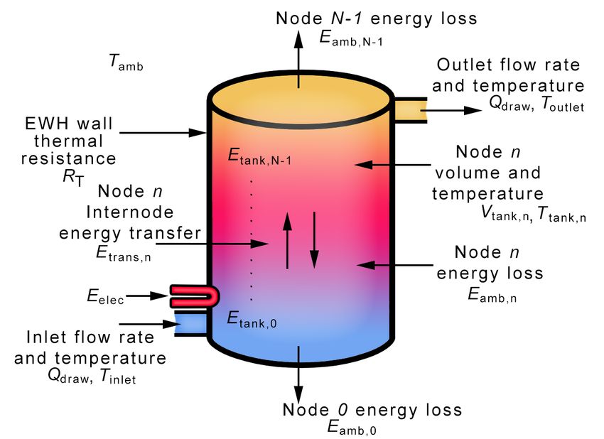
Figure 1b shows a diagram of the multi-node EWH model. The significant change from the one-node
model is that the temperature of the tank is modelled as a vertical gradient. The body of water is split into
N nodes stacked on top of each other. At node n, the temperature of the water is always higher or equal to
4(a) (b)
Figure 1: Energy flow, thermal resistance, flow rate, temperature and volume in a) a single node and b) multi-node EWH.
that of the lower node at n − 1. Water drawn from the tank is at the temperature of the top node, N − 1 and
cold water enters the bottom node 0. The heating element also supplies electrical energy to this node. For
each node, the standing losses occur at the segment of the tank that surrounds that node and is dependent
on the water temperature of the node, Ttank, n . Water stratification occurs at every boundary of two adjacent
nodes due to the temperature difference. The internode energy transfer at a node, Etrans,n , occurs at a rate
determined by the thermal resistance of the thermocline.
The thermal dynamics for each node of the multi-node EWH model is described as follows:
Pelec (t) + Pinlet (t) − Pflow,n-1 (t) + Pinv,n+1 (t) − Ploss,n (t) if n = 0
Ėtank,n (t) = −Pflow,n-1 (t) − Ploss,n (t) − Pinv,n-1 (t) if n = N − 1 (1)
−Pflow,n-1 (t) − Ploss,n (t) − Pinv,n-1 (t) − Pinv,n+1 (t) otherwise
where Etank,n (t) is the thermal energy in node n, Pelec is the electrical energy supplied by the heating element,
Pflow,n-1 is the power transfer of mass flow due to buoyancy, Pinv,n-1 and Pinv,n+1 is the water stratification
that occurs between the adjacent nodes, Ploss,n (t) is the power leaving node n due to losses to the environment,
and n = 0 and n = N − 1 refers to the top and bottom nodes.
The thermal energy of the tank is calculated as the sum of energy in each node, and is calculated as
follows:
N
X −1
Etank (t) = Etank,n (t) (2)
n=0
When water is drawn from the top of the tank and replaced with cold water at the bottom, a mass flow
occurs due to buoyancy and the transfer of thermal energy in each node is calculated as follows:
Pflow,n (t) ≈ cρQdraw (t)Ttank,n-1 (t) (3)
where c is the constant volume-specific heat capacity, ρ is the density of water, and Ttank,n-1 is the temperature
of the water inside the lower adjacent node. The power loss from each node to the environment is calculated
as follows:
1
Ploss,n (t) = [T tank,n (t) − Tamb (t)] (4)
RT,n
5where RT,n is the thermal resistance of the wall that is occupied by node n, and Ttank,n is the temperature of
the water in node n. If there is a temperature difference between node n and any adjacent node, the power
transfer from node n to the adjacent nodes is calculated as follows:
1
Pinv,n-1 (t) = [T tank,n (t) − Ttank,n-1 (t)] (5)
RTH
1
Pinv,n+1 (t) = [T tank,n (t) − Ttank,n+1 (t)] (6)
RTH
The relationship between the node energy, Etank,n , and the node water temperature relative to a reference
temperature, where we define energy to be zero, is given as follows:
E tank,n (t)
T tank,n (t) ≈ (7)
cρVtank,n
where Vtank,n is the volume of node n.
4.2. Optimisation Algorithm
The optimal temperature and heating planning for the multi-node EWH are produced by an A* search
algorithm. The algorithm was previously formulated for a stratified two-node EWH model by Engelbrecht
et al. (2021) and is modified in this study to produce the optimal planning for a multi-node EWH.
Optimal control problem
The optimal control problem is to determine the optimal switching sequence of the heating element to
minimise the total electrical energy supplied to the EWH while satisfying a given hot water usage profile.
The profile is satisfied if the user never experiences a temperature below the minimum usage temperature,
Tusage , when hot water is drawn from the tank.
The system dynamics are defined by the differential equations that describe the thermodynamics of the
multi-node EWH, specified by equations (1), (2), (3), (4), (6) and (7). The system states is represented by
x(t) and is defined by the thermal energy in each node. The state vector is defined as follows:
T
x(t) = Etank,0 (t) Etank,1 (t) ... Etank,N-1 (t) (8)
The state constraints are defined by the physical limitations of the thermal energy of the tank. For node
n, the lower and upper bounds are represented by Emin,n and Emax,n . These correspond to the minimum
and maximum admissible temperatures, Tmin,n and Tmax,n , with a constant volume of Vtank,n .
The control input is represented by u(t) and is defined as Pelec , the electrical power supplied by the
heating element. The control input is constrained to supply power equal to either zero or Prated , the power
rating of the heating element.
The cost function has the objective of minimising the electrical energy and is defined as follows:
Z tf
J= Pelec (t)dt (9)
ti
where ti and tf is the initial and final time instant. Temperature profile constraints are defined for each node
to ensure that the hot water usage profile is satisfied. The following inequality represents the objective of
the temperature of each node to satisfy the hot water usage profile:
Ttank,n (t) ≥ Tprofile,n (t) (10)
where Tprofile,n are the constraints imposed on node n and is expressed as follows:
6
Tusage if Qdraw (t) > 0
Tprofile,n (t) = TLegionella once per day (11)
Tmin,n otherwise
where TLegionella is the temperature required to prevent the growth of Legionella. These constraints show that
the outlet water temperature cannot fall below Tusage during water usage, the entire tank must be sufficiently
heated to ensure Legionella prevention, and the temperature of the tank cannot exceed the minimum EWH
temperature, Tmin .
A* search algorithm
The A* search algorithm is a shortest path search algorithm that is popular and widely used. The
algorithm can solve non-linear optimal control problems by creating multiple node-based paths that originate
at a starting position, and each one navigates towards a desired final position. The algorithm performs
efficiently as heuristics are introduced to help optimise the decision making of the process.
Before the A* search algorithm can be applied to the optimal control problem, it is required that the
problem is discretised into discrete time instants and states to represent the decision stages and choices,
respectively. Since the hot water usage data is presented with one-minute resolution, equations (1), (2), (3),
(4), (6) and (7) are discretised with a minutely sampling period ∆t.
The purpose of the algorithm is to find the shortest path from an initial state at time instant ti to a
goal state at time instant tf . At the initial state, the temperature of the entire tank is assumed to be at
the starting temperature Tstart . At the goal state, the temperature of the entire tank must greater than or
equal to the final temperature Tend . Tstart and Tend are the boundary conditions for the optimal path and
are specified for the algorithm.
A binary search tree (BST) data structure is defined to aid the navigation of the search process (more
information on the BST data structure can be found in Nagaraj (1997)). The BST comprises multiple search
paths that extend from the initial state and navigate to the final state. The paths are made up of nodes
connecting states in the previous time instants to the calculated state in the next time instant as a result of
the scenarios where the control input u = 0 and u = 1.
Each search path ending calculates a cost that is the sum of two components: the amount of electrical
energy that was required to reach its current position and the estimated amount of electrical energy that is
still required to reach the final state at the last time instant. A priority queue keeps track of the cost of every
path ending, prioritises them from lowest to highest cost, determines which path end is currently the closest
(and most optimal path) from the desired final state, and instructs that path to extend further.
The first path that reaches the desired state at the last time instant is also the optimal path and the
algorithm finishes executing. With the optimal path acquired, the optimal temperature trajectory and heating
schedule is produced for the given hot water usage profile.
4.3. Heating control strategies
Three heating control strategies are presented in this study:
Thermostat Control (TC): This is the baseline strategy that is used to evaluate the energy savings achieved
by the following two methods. This strategy represents how the EWH typically operates and is vastly ineffi-
cient. The water temperature is maintained at the set-point temperature of the thermostat. Therefore, high
standing losses are expected as the tank is always hot, even when water is not drawn for long periods.
Temperature-matched optimal control (TM): This strategy is produced by the A* search algorithm and de-
termines the optimal control of the EWH for a given hot water usage profile. However, the temperature
profile constraints are modified such that the temperature of the tank at the start of water usage is exactly
matched to the temperature that is expected in the scenario where the same water usage occurs for TC. This
strategy ensures that the temperature and energy of the water drawn from the EWH is not compromised by
the reduction in electrical energy that is supplied.
7Energy-matched optimal control with Legionella prevention (EML): This strategy is similar to the previous
strategy, except that the temperature is only constrained to Tusage during water usages. However, the hot
water flow rate is increased during water usages to ensure that an equivalent amount of energy is delivered,
despite the lower temperature experienced by the user. A lower temperature profile can cause the growth of
Legionella inside the tank and introduce a health risk. This problem is mitigated by ensuring that the EWH
is heated to TLegionella at least once a day to prevent the growth of Legionella.
5. Simulation Results
The simulations results for the TM and EML heating control strategies are summarised in Table 2 and
3, respectively.
Figure 2 shows the 4-node EWH simulation results for the temperature-matching and energy-matching
with Legionella prevention heating control strategies for the same 24-hour hot water profile (shown in blue).
The plot shows the temperature profile for all four nodes, the state of the heating element Pelec (shown in
red), and the minimum usage temperature Tusage of 40°C (shown in black). The temperature profile of the
highest node for TC is also shown. All simulations started with the temperature of the whole tank at the
set-point temperature (68.5°C) at the beginning of the first day. However, the observed day in the figures is
not the first day of the simulation and the state of the EWH at the start of day may vary.
(a) Temperature-matching (b) Energy-matching with Legionella prevention
Figure 2: Simulation results of a 4-node EWH for optimal temperature matching and energy matching with Legionella prevention.
The plots show the temperature of each node, the outlet flow rate, and the heating element state (either a value of zero or
the rated power of 3 kW). The temperature profile of the highest node for thermostat control is repeated on each plot with a
segmented black line. The minimum usage temperature of (40°C) is shown by with a solid black line on each plot.
Thermostat Control (TC): The thermostat keeps the temperature of the tank at the set-point temperature
of 68.5°C and allowing for 1.5°C hysteresis. The heating element switches on when the temperature falls below
67°C and switches off again once the temperature has risen to 70°C. The electrical energy used for TC was
8.7 kWh.
Optimal temperature matching (TM): As shown in Figure 2a, this strategy ensures that the temperature
of the whole tank is equal to that of TC at the start of each water usage. This means that the heating element
only switches on just before the start of a water usage and won’t turn on again until the next usage. This
results in the temperature being lower than TC during the period between usages. By observing the water
usage at 7am, the heating element increases the water temperature until the temperature reaches that of TC
right before the usage occurred. During the usage, cold water mixes with the lowest node and the dropped to
44°C. Following this, the temperature of all the nodes exponentially converge to a single temperature until
8the heating element is switched on again in preparation for the next water usage that occurs at 6pm. The
electrical energy used for TM was 6.25 kWh.
Optimal energy matching with Legionella prevention (EML): As shown in Figure 2b, this strategy ensures
that the temperature of the whole tank remains above 40°C during water usage. Despite a outlet temperature
lower than TC, the flow rate is increased during usage to ensure that the equivalent amount of thermal energy
is delivered. This simulates the fact that the user will adjust the mixing of hot and cold water to allow for
more hot water to leave the tank. By observing the water usage at 7am, it can be seen that the maximum
flow rate increased form 5 to 19 L/min. This strategy also ensures the prevention of Legionella by heating
the whole tank to 60°C for at least 11 minutes. By observing the water usage at 6pm, it can be seen that
this occurred right before the usage. The electrical energy used for EML was 5.25 kWh.
Figure 3 shows the temperature planning for TC of the bottom node for a 24-hour hot water usage profile
(shown in dark blue) for M = 2, 4, 10 and 20. The inlet water temperature, Tinlet , is marked with a black
segmented line on each figure.
Figure 3: Plots of the temperature profile for the bottom node for TC when the EWH is modelled with M = 2, 4, 10 and 20.
The 24-hour hot water usage profile (dark blue) is repeated on each plot and Tinlet is marked with a black segmented line.
Comparing these sub-figures, the water temperature of the node decreases to a lower temperature during
water usage when the number of nodes M is increased. This is because a bigger portion of the lower nodes
is mixed with the cold inlet water because the volume of each node is smaller. For M = 20, it can be seen
that the bottom nodes temperature does not drop below Tinlet . This figure is important for understanding
the optimal planning of the EWH for more nodes and aids the analysis of the simulation results presented
next.
Looking at the results for TM in Table 2, the control strategy for all values of M was successful in
matching the temperature during water usages and delivering the same amount of energy as the baseline
strategy. The key difference in the results for the different number of nodes is observed in the daily energy
losses. The daily standing losses decreased as M increased. As seen from Figure 3, the optimal temperature
plan for M nodes will expect the temperature of the bottom node to decrease less when M is lower than
N . Therefore, the temperature feedback controller will ensure that the 20-node EWH follows a temperature
plan that is higher between water usages and resulting in higher standing losses. For M = 20, the achieved
energy savings, given as [25th percentile, median, 75th percentile], of [3.14, 6.24, 11.51 ] % (or [0.30, 0.44,
0.60 ] kWh/day) was obtained for TM. The results for M = 20 showed the best performance because the
temperature feedback controller is not required for the simulated EWH temperature to follow the optimal
trajectory.
Looking at the results for EML in Table 3, the same trend occurs as M increases. The difference is that
the daily average usage temperature decreased to 56°C. This is because the temperature does not need to
match the temperature of the baseline condition during water usages, and must only remain about Tusage .
The best energy savings of [11.21, 16.30, 21.02 ] % (or [0.82, 1.05, 1.34 ] kWh/day) was achieved by the
9Figure 4: Daily energy reduction reduction in electrical energy for various values of M for TM (green) and EML (orange). The
solid lines represent the median savings achieved by an EWH for a day. The segmented lines represent the corresponding 25th
and 75th percentiles for each strategy.
20-node EWH model for EML.
Figure 4 shows the daily reduction in electrical energy for the median energy savings (solid line) and the
25th and 75th percentiles (segmented lines) for using different values of M for TM (green) and EML (orange).
The energy-saving plots for both TM and EML show that the energy savings significantly decrease for using
lower values of M , and the gradient flattens after M = 4. This suggests that determining the optimal control
of a multi-node EWH can obtain sufficiently accurate results by using four nodes and anything more than
this produces diminishing returns.
Table 2: Daily temperature-matched simulation results for increasing the nodes of the EWH during the planning and simulating
on a 20-node EWH.
No. of Tusage Electricity Energy Energy Energy Savings Energy Savings (%)
nodes Used Used Loss (kW h/day)
(M ) (kW h/day) (kW h/day) (kW h/day)
1 68.6 7.12 4.68 2.18 0.01, 0.06, 0.13 0.15, 0.93, 2.01
2 68.3 6.98 4.68 2.03 0.02, 0.15, 0.34 0.31, 2.31, 5.25
3 68.1 6.89 4.68 1.97 0.14, 0.23, 0.39 2.16, 3.55, 6.02
4 68.2 6.85 4.68 1.96 0.18, 0.31, 0.45 2.78, 4.78, 6.94
5 68.2 6.80 4.68 1.94 0.19, 0.32, 0.48 2.93, 4.94, 7.41
6 68.2 6.75 4.68 1.94 0.20, 0.33, 0.48 3.09, 5.09, 7.41
8 68.2 6.75 4.68 1.93 0.21, 0.34, 0.49 3.24, 5.25, 7.56
10 68.2 6.75 4.68 1.93 0.21, 0.34, 0.49 3.24, 5.25, 7.56
14 68.1 6.80 4.68 1.92 0.21, 0.35, 0.49 3.24, 5.40, 7.56
20 68.7 6.65 4.68 1.83 0.30, 0.44, 0.60 4.63, 6.79, 9.26
Note: The distributions are reported as 25th percentile, median, 75th percentile
6. Conclusion
In this paper, we determine the best energy savings that can be achieved by modelling the EWH as
multi-nodal and providing it with optimal control with perfect foreknowledge of the hot water usage profile.
The average daily energy savings achieved for 77 household’s over one month was 6.24 % (0.44 kWh/day)
for temperature-matched and 16.30 % (1.05 kWh/day) for energy-matched optimal control of the heating
element.
Furthermore, we also evaluated how increasing the number of nodes of the EWH when calculating the
optimal heating schedule affected the energy savings. It was determined that increasing the nodes resulted
10Table 3: Daily energy-matched simulation results for increasing the nodes of the EWH during the planning and simulating on
a 20-node EWH.
No. of Tusage Electricity Energy Energy Energy Savings Energy Savings (%)
nodes Used Used Loss (kW h/day)
(M ) (kW h/day) (kW h/day) (kW h/day)
1 56.5 6.20 4.65 1.43 0.74, 0.86, 0.99 11.42, 13.27, 15.27
2 56.1 6.15 4.64 1.38 0.80, 0.91, 1.05 12.34, 14.04, 16.20
3 56.0 6.10 4.64 1.34 0.80, 0.94, 1.11 12.34, 14.50, 17.13
4 56.0 6.05 4.64 1.33 0.81, 0.98, 1.17 12.50, 15.12, 18.05
5 56.0 6.05 4.64 1.32 0.81, 0.98, 1.18 12.50, 15.12, 18.21
6 55.9 6.05 4.64 1.32 0.81, 0.99, 1.21 12.50, 15.27, 18.67
8 56.0 5.95 4.62 1.32 0.81, 0.99, 1.23 12.50, 15.27, 18.98
10 56.0 5.93 4.63 1.32 0.81, 0.99, 1.24 12.50, 15.27, 19.13
14 56.3 5.95 4.63 1.32 0.79, 1.01, 1.26 12.19, 15.58, 19.44
20 56.0 5.78 4.64 1.26 0.82, 1.05, 1.34 12.65, 16.20, 20.67
Note: The distributions are reported as 25th percentile, median, 75th percentile
in smaller standing losses between water usages and improving the savings. We concluded that the extent of
improvement is negligible if more than four nodes are used.
In future work, the computational complexity of simulations and algorithms for producing accurate out-
comes can be greatly reduced if a 4-node EWH model is used.
Acknowledgment
We thank the following organisations for funding: MTN (S003061) and the WRC (K1-7163), and Eskom
(TESP-2019).
References
Armstrong, P.M., Uapipatanakul, M., Thompson, I., Ager, D., McCulloch, M., 2014. Thermal and sanitary
performance of domestic hot water cylinders: Conflicting requirements. Applied Energy 131, 171 – 179.
doi:10.1016/j.apenergy.2014.06.021.
Booysen, M., Engelbrecht, J., Ritchie, M., Apperley, M., Cloete, A., 2019a. How much energy can optimal
control of domestic water heating save? Energy for Sustainable Development 51, 73–85.
Booysen, M.J., Cloete, A.H., 2016. Sustainability through intelligent scheduling of electric water heaters in
a smart grid, in: 2016 IEEE 2nd Intl Conf on Big Data Intelligence and Computing and Cyber Science
and Technology Congress, pp. 848–855. doi:10.1109/DASC-PICom-DataCom-CyberSciTec.2016.145.
Booysen, M.J., Visser, M., Burger, R., 2019b. Temporal case study of household behavioural response to
Cape Town’s “Day Zero” using smart meter data. Water Research 149, 414–420.
Bridgiot, . Geasy - a smart geasy controller by bridgiot. https://www.bridgiot.co.za/solutions/
geasy-2/. Accessed: 2019-09-17.
Dongellini, M., Falcioni, S., Morini, G.L., 2015. Dynamic simulation of solar thermal collectors for domestic
hot water production. Energy Procedia 82, 630–636. doi:10.1016/j.egypro.2015.12.012.
Engelbrecht, J., Ritchie, M.J., Booysen, M., 2021. Optimal schedule and temperature control of stratified
water heaters. Energy for Sustainable Development 62, 67–81.
Ericson, T., 2009. Direct load control of residential water heaters. Energy Policy 27, 3502–3512. doi:DOI:
10.1016/j.enpol.2009.03.063.
ESKOM, 2021. URL: https://loadshedding.eskom.co.za/loadshedding/description.
11Fernández-Seara, J., Uhı́a, F.J., Sieres, J., 2007. Experimental analysis of a domestic electric hot water
storage tank. part i: Static mode of operation. Applied Thermal Engineering 27, 129–136. URL: https:
//doi.org/10.1016/j.applthermaleng.2006.05.006, doi:10.1016/j.applthermaleng.2006.05.006.
Gato, S., Jayasuriya, N., Roberts, P., 2007. Forecasting residential water demand: Case study. Journal of
Water Resources Planning and Management 133, 309–319.
Gerin, O., Bleys, B., De Cuyper, K., 2014. Seasonal variation of hot and cold water consumption in apartment
buildings, in: Proceedings of CIB W062, 40th International Symposium on Water Supply and Drainage
for Building (Sao Paulo, Brazil,), pp. 1–9.
Gholizadeh, A., Aravinthan, V., 2016. Benefit assessment of water-heater management on residential demand
response: An event driven approach, in: 2016 North American Power Symposium (NAPS), pp. 1–6.
doi:10.1109/NAPS.2016.7747831.
Hohne, P., Kusakana, K., Numbi, B., 2019. A review of water heating technologies: An application to the
South African context. Energy Reports 5, 1–19. doi:10.1016/j.egyr.2018.10.013.
Jamie McKane, 2021. Ramaphosa announces plan to save Eskom and
stop load-shedding. URL: https://mybroadband.co.za/news/energy/
386264-ramaphosa-announces-plan-to-save-eskom-and-stop-load-shedding.html.
Kepplinger, P., Huber, G., Petrasch, J., 2015. Autonomous optimal control for demand side management
with resistive domestic hot water heaters using linear optimization. Energy and Buildings 100, 50 – 55.
doi:https://doi.org/10.1016/j.enbuild.2014.12.016.
Kepplinger, P., Huber, G., Preißinger, M., Petrasch, J., 2019. State estimation of resistive domestic hot water
heaters in arbitrary operation modes for demand side management. Thermal Science and Engineering
Progress 9, 94–109.
Mabina, P., Mukoma, P., Booysen, M., 2021. Sustainability matchmaking: Linking renewable sources to
electric water heating through machine learning .
Mathu, K., 2017. Cleaning South Africa’s coal supply chain. Journal of Business Diversity 17. doi:10.33423/
jbd.v17i3.1236.
Nagaraj, S., 1997. Optimal binary search trees. Theoretical Computer Science 188, 1–44.
Nejat, P., Jomehzadeh, F., Taheri, M.M., Gohari, M., Majid, M.Z.A., 2015. A global review of energy
consumption, co2 emissions and policy in the residential sector (with an overview of the top ten co2
emitting countries). Renewable and sustainable energy reviews 43, 843–862.
Nel, P.J.C., 2015. Rethinking electrical water heaters. Master’s thesis. Stellenbosch: Stellenbosch University.
Nel, P.J.C., Booysen, M.J., van der Merwe, A.B., 2016. A computationally inexpensive energy model for
horizontal electric water heaters with scheduling. IEEE Transactions on Smartgrid doi:10.1109/TSG.2016.
2544882.
Pomianowski, M.Z., Johra, H., Marszal-Pomianowska, A., Zhang, C., 2020. Sustainable and energy-efficient
domestic hot water systems: A review. Renewable and Sustainable Energy Reviews 128, 109900.
Ritchie, M., Engelbrecht, J., Booysen, M., 2021a. A probabilistic hot water usage model and simulator for
use in residential energy management. Energy and Buildings 235, 110727.
Ritchie, M.J., Engelbrecht, J.A., Booysen, M.J., 2021b. Practically-achievable energy savings with the optimal
control of stratified water heaters with predicted usage. Energies 14, 1963.
Roux, M., Booysen, M.J., 2017. Use of smart grid technology to compare regions and days of the week in
household water heating, in: 2017 International Conference on the Domestic Use of Energy (DUE), IEEE.
pp. 276–283. doi:10.23919/DUE.2017.7931855.
12Siegel, J.E., Das, A., Sun, Y., Pratt, S.R., 2020. Safe energy savings through context-aware hot water demand
prediction. Engineering Applications of Artificial Intelligence 90, 103481.
Skinner, T., et al., 2012. An overview of energy efficiency and demand side management in South Africa, in:
Presentation to the world bank/IFC workshop on appropriate incentives to deploy renewable energy and
energy efficiency, Washington, DC. Available online: www. eskom. co. za.
Spur, R., Fiala, D., Nevrala, D., Probert, D., 2006. Influence of the domestic hot-water daily draw-off profile
on the performance of a hot-water store. Applied Energy 83, 749–773. doi:10.1016/j.apenergy.2005.
07.001.
Stone, W., Louw, T.M., Gakingo, G.K., Nieuwoudt, M.J., Booysen, M.J., 2019. A potential source of
undiagnosed legionellosis: Legionella growth in domestic water heating systems in south africa. Energy for
Sustainable Development 48, 130–138. doi:10.1016/j.esd.2018.12.001.
Stout, J.E., Best, M.G., Yu, V.L., 1986. Susceptibility of members of the family legionellaceae to thermal
stress: implications for heat eradication methods in water distribution systems. Applied and environmental
microbiology 52, 396–399. doi:10.1016/j.semcdb.2010.11.003.
Xiang, S., Chang, L., Cao, B., He, Y., Zhang, C., 2019. A novel domestic electric water heater control
method. IEEE Transactions on Smart Grid .
Zhou, S., McMahon, T., Walton, A., Lewis, J., 2002. Forecasting operational demand for an urban water
supply zone. Journal of hydrology 259, 189–202.
13You can also read