LECTURE 12: LOCOMOTION - GITHUB
←
→
Page content transcription
If your browser does not render page correctly, please read the page content below
EE 290-005 Integrated Perception, Learning, and Control                                     Spring 2021

                                     Lecture 12: Locomotion
                                                Scribes: Ayush Agrawal, Fernando Castañeda, Jason Choi

12.1      State Estimation

12.1.1     Introduction

State estimation is an important complement to the control problem because once we get an accurate and
reliable estimation of the robot’s state, the control gets much easier.
Two recent papers [1, 2] are introduced that tackle mobile robot state estimation for legged robots, or more
specifically all robots that may involve contact with the environment.
Although there have been many recent advancements in visual–inertial odometry and simultaneous local-
ization and mapping, these algorithms often rely on visual data for pose estimation. This means that the
observer (and ultimately the feedback controller) can be adversely affected by rapid changes in lighting as
well as the operating environment. It is therefore beneficial to develop a low-level state estimator that fuses
data only from proprioceptive sensors to form accurate high-frequency state estimates.
Nearly all ground mobile robots contact with the ground, from wheel-based vehicles whose wheels touch the
ground almost all the time to all kinds of legged robots.
One of the motivations of these two papers is that these robots make periodic contact with the ground, and
in the meantime, slip is ideally excluded for the agent to have more reliable locomotion. The contact points
can largely be assumed to be fixed on the ground.

12.1.2     Invariant Extended Kalman Filter (InEKF)

Invariant observer: observer whose estimation error being invariant under the action of a matrix Lie group
[3, 4].

   • State defined on a Lie group and dynamics satisfying a particular group-affine property
   • Symmetry leads to the estimation error satisfying a log-linear autonomous differential equation on the
     Lie algebra
   • In the deterministic case, this linear system can be used to exactly recover the estimated state of the
     nonlinear system as it evolves on the group.
   • Log-linear property, therefore, allows the design of a nonlinear observer or state estimator with strong
     convergence properties.
Invariant EKF: The author derived an invariant extended Kalman filter (InEKF) for a system containing
IMU and contact sensor dynamics, with forward kinematic correction measurements.

   • IMU (gyroscope and accelerometer)
   • Contact (force sensor, or estimated from motor torque)
   • Kinematics (joint encoder)

                                                     12-1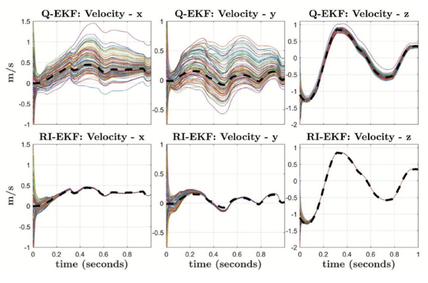
12-2                                                                               Lecture 12: Locomotion

Figure 12.1: Invariant EKF (InEKF) versus Quaternion EKF (QEKF). The choice of error variables is the
main difference between the InEKF and the QEKF. Instead of the right-invariant error, QEKF typically
uses decoupled error states. Video link: https://youtu.be/pNyXsZ5zVZk

12.1.3    Contact-aided state estimation combined with vision
In the second paper [2], the authors combine contact-aided state estimation and vision into a factor-graph
optimization framework. In the factor graph, the states are the nodes and the measurements are the factors.
Nodes are added to the graph every time a contact is made or removed. The authors introduce Hybrid
Contact Pre-integration which allows contacts to be integrated through an arbitrary number of contact
switches. This leads to the reduction in the number of variables in the nonlinear optimization problem.

Figure 12.2: Contact switches (left): when the foot is on the ground, the contact frame remains fixed on
the ground with respect to the world frame. The estimator returns SE(3) pose of the base frame. Factor
graph framework (right): The robot’s state along a discretized trajectory is denoted by red circles. Each
independent sensor measurement is a factor denoted by lines that constraints the state at separate time-
steps. The proposed hybrid contact factor (shown on top) allows pre-integration of high-frequency contact
data through an arbitrary number of contact switches. In this example, there are two contact switches,
where the robot moves from left-stance (L) to right-stance (R), then back to left stance. The pink factor
indicates constraints brought by the camera measurements. The depth image from the camera makes sure
the consistency of the landmarks. The forward kinematic constraints are indicated in purple.
Lecture 12: Locomotion 12-3
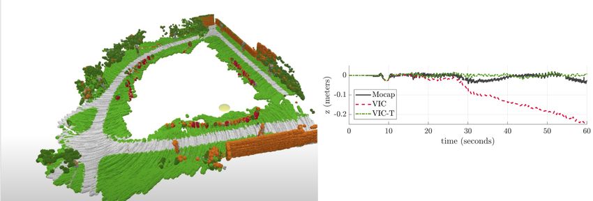
Figure 12.3: Experiment of contact-aided vision-based state estimation and mapping. Snapshot of the video
(left, link: https://youtu.be/uFyT8zCg1Kk): In the video, image defects such as motion blur are caused by
the vibration of the robot. In the scene, the author assumed that there are no moving objects like humans.
The plot on the right shows how a locked axis can help with the state estimation. The red dashed line shows
the estimated trajectory without locking the z-axis, thus, it drifts. When the robot is reliably attached to
the ground and the z-direction placement is never negative, by trusting the z-axis kinematics of the robot,
a more accurate estimate can be generated (green line).
12.2 Model-based Control For Locomotion
There have been several model-based control strategies developed for legged locomotion, including Model-
Predictive Control, controllers based on simple inverted pendulum models, as well as controllers based on
the full nonlinear dynamics of the robot such as hybrid zero dynamics based control.
12.2.1 Model-based Control for Quadrupeds
Model Predictive Control (MPC)-based Method [5]
In [5], the authors propose an MPC-based method for controlling the MIT Cheetah 3, a quadrupedal robot
that weighs about 45kg with three torque controlled joints at each leg - one each for hip abduction/adduction,
hip pitch and knee pitch. The mass of the legs for the Cheetah 3 accounts for only 10% of the robot’s total
mass, this allows the authors to ignore the leg dynamics for the purpose of control design. As illustrated in
Fig. 12.4, the robot is modelled as a single rigid body with control inputs as the ground reaction forces fi
at the foot. The rigid body dynamics is given by
Σni=1 fi
p̈ = − g, (12.1)
m
d
(Iω) = Σni=1 ri × fi , (12.2)
dt
Ṙ = [ω]× R, (12.3)
where p is the robot’s center-of-mass position, fi are the reaction forces between the ith foot and the ground,
ri is the location of the ith foot from the robot’s center-of-mass position, R ∈ SO(3) is the rotation matrix
representation of the orientation of the robot, and ω is the body angular velocity of the robot. In addition to
simplifying the dynamics of the robot, the rigid-body model captures the necessary inputs to the system - the
only external forces acting on the robot (and thus affecting its acceleration) are the ground reaction forces at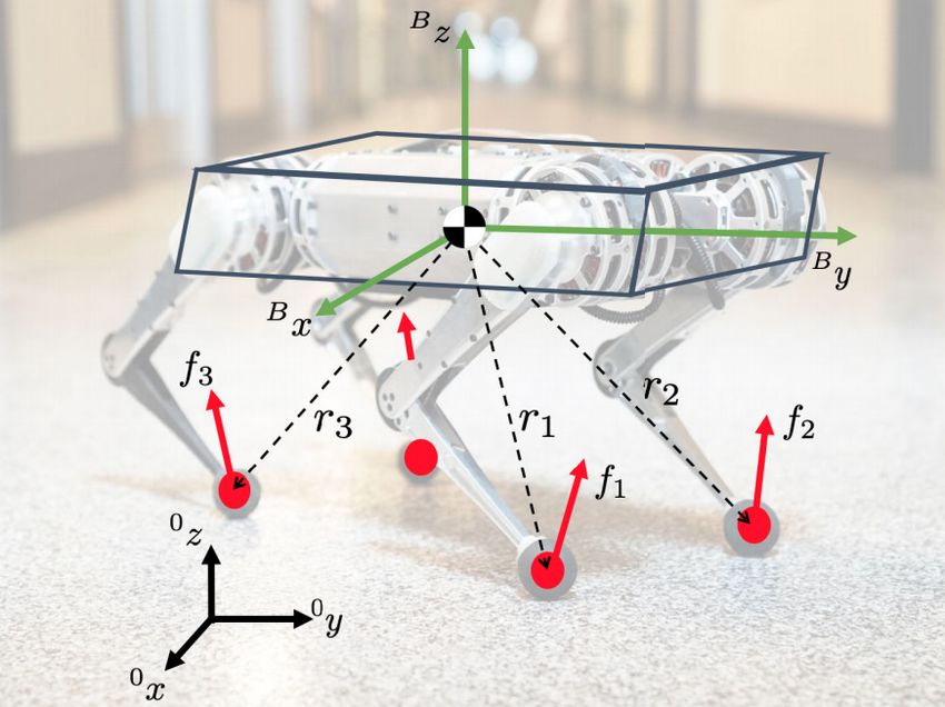
12-4 Lecture 12: Locomotion
Figure 12.4: Rigid-body model of the minicheetah robot. The only source of external forces acting on the
robot are the ground reaction forces at the feet.
the feet contacting the ground. However, as seen in (12.2) and (12.3), rigid-body dynamics corresponding to
the orientation of the robot are nonlinear, which would make the resulting model-predictive control problem
non-convex. In order to further simplify the problem, the authors make an assumption of small roll and
T
pitch angles which enables them to linearize the orientation dynamics. In particular, if [φ θ ψ] denotes the
Z − Y − X euler angle representation of the orientation of the robot, then the relationship between the euler
angle rates and the body angular velocities is given by
φ̇ cos(ψ)/ cos(θ) sin(ψ)/ cos(θ) 0
θ̇ = − sin(ψ) cos(ψ) 0 ω, (12.4)
ψ̇ cos(ψ) tan(θ) sin(ψ) tan(θ) 1
which is nonlinear in the pitch φ and roll θ. However, with the assumption of small roll and pitch angles,
the following relationship between the euler angle rates and body angular velocity is obtained,
φ̇ cos(ψ) sin(ψ) 0
θ̇ = − sin(ψ) cos(ψ) 0 ω, (12.5)
ψ̇ 0 0 1
| {z }
RzT (ψ)
which allows the orientation dynamics in (12.2) to be approximated as
d
(Iω) ≈ I ω̇. (12.6)
dt
The robot dynamics can then be written as,
ẋ(t) = Ac (ψ)x(t) + Bc (r1 , r2 , r3 , r4 , ψ)u(t), (12.7)
h iT
where the state vector x = Θ p Θ̇ ṗ denotes the orientation and center-of-mass position and velocities of
the robot and the control inputs u(t) denote the ground contact forces fi . This form of the dynamics only
depends on the foot-step locations ri and the yaw of the robot ψ, which can be computed ahead of time and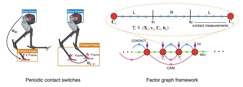
Lecture 12: Locomotion                                                                                     12-5

the resulting dynamics become time-varying and linear. This allows for the implementation of the MPC as
a quadratic program (12.8) that can be implemented on hardware at 30Hz,
                                         Pk−1
                                   minx,u i=0 kxi+1 − xi+1,ref kQi + kui kRi
                             subject to xi+1 = Ai xi + Bi ui , i = 0 . . . k − 1                  (12.8)
                                              ci ≤ Ci ui ≤ ci , i = 0 . . . k − 1
                                                   Di ui = 0, i = 0 . . . k − 1,

where xi,ref denotes the reference state-trajectory which is obtained from user input commands. In addition
to the desired state-trajectory xi , The MPC outputs desired contact forces ui for the feet that are in contact
with the ground. The constraints in the MPC includes friction constraints and unilateral ground reaction
force constraints (i.e. the ground cannot pull the robot’s feet) as in (12.9), in addition to the dynamics
constraints.
                                                fmin ≤ fz ≤ fmax
                                              −µfz ≤ ±fx ≤ µfz                                           (12.9)
                                              −µfz ≤ ±fy ≤ µfz

To obtain the resulting joint-torques of the leg in contact with the ground, the following static map is used,
                                                    τi = JTi fi ,                                       (12.10)

where Ji ∈ R3×3 is the body-jacobian of the ith contacting foot and τi ∈ R3 are the joint torques.
To obtain the joint torques of the legs that are not in contact with the ground, a heuristic foot-placement
controller is implemented that aims to stabilize the robot’s velocity. The reference swing feet positions pi,ref
and velocities vvi,ref are tracked using an impedence controller (12.11),
                             τi = J>
                                   i [Kp (pi,ref − pi ) + Kd (vi,ref − vi )] + τ i,ff ,                 (12.11)

where τ i,ff denotes the feedforward torques computed using the desired acceleration of the feet as,


                                  τ i,ff = J> Λi ai,ref − J̇i q̇i + Ci q̇i + Gi ,                       (12.12)

where Λi is the operational space inertial matrix, ai,ref is the reference acceleration of the foot, qi is the
vector of joint positions, and Ci + Gi is the torque due to gravity and Coriolis forces for the leg. The overall
control architecture is illustrated in Fig. 12.5.
MPC using Variation-Based Linearization [6]
The method presented in the previous section made use of a small-angle approximation to obtain a linear
time-varying dynamics. This, however, limits the capabilities of the robot and prevents it from achieving
more dynamics tasks where the small-angle approximation assumption breaks. However, by noting the fact
that the orientation of the robot R belongs to the special orthogonal group SO(3), one can take the variation
with respect to a desired trajectory Rbd on the SO(3) manifold, as
                                             d
                                                        Rbd exp B ηb = RbdB ηb,

                                     δRb =                                                              (12.13)
                                             d   =0

where B η ∈ R3 is an approximation of the angle-axis error describing the rotation necessary to achieve
the desired orientation and the exponential map maps a skew-symmetric matrix to a rotation matrix. The
variation can be thought of as a local approximation of the displacement between two points on a manifold.
The variation in angular velocity can be obtained as,
                                              δB ω = B ω
                                                       b dB η + B η̇.                                   (12.14)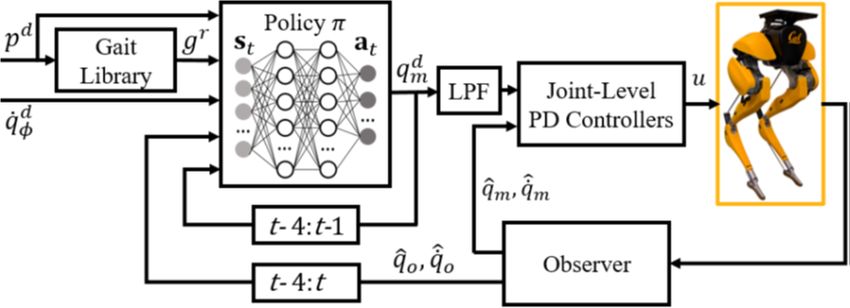
12-6 Lecture 12: Locomotion
Figure 12.5: Control diagram of the Cheetah 3 MPC-based control. The MPC controller takes as inputs
the user reference trajectories in the form of desired velocities and contact sequence c and outputs desired
contact forces fi for the stance foot. A heuristic foot-placement controller outputs the desired swing-feet
positions, velocities and accelerations to stabilize the robot. Blocks shaded blue run at 30 Hz, blocks shaded
red run at 1 kHz, and blocks shaded green run at 4.5 kHz.
Using the following formulas for taking variations,
δ(x + y) = δx + δy (12.15)
δ(x × y) = δx × yd + xd × δy
δ(x · y) = δx · yd + xd · δy
δ (R1 x) = δR1 xd + R1,d δx
δ (R1 R2 ) = (δR1 ) R2,d + R1,d (δR2 )
the linear variation dynamics of the rigid-body (12.1)-(12.3) can be obtains as
pc − pdc
Pδ ṗ
δp δpc ep
d
1
δfi − g ṗc − ṗdc
Bδ ṗ =
m
δ ṗc ev
∨
η ≈
, s :=
=
−B ω dB η + δ B ω
T
Rbd Rb − RbT Rbd
1
dt η eR
T P 2
B −1
δRbT δB ω
P d
B
δ ω I τi + Rbd δτi − c eω B
ω−
B
RbT Rbd ω d
(12.16)
which results in the linear system of equations for the error-dynamics,
···
03 I3 03 03 03 03
1 1
03 03 03 03 m I3 ··· m I3
A= b d
,B =
03 ··· 03
(12.17)
03 03 −Bω I3
T T
A4,1 03 A4,3 A4,4 B −1
I Rbd rb1 d ... B −1
I Rbd rb4d
T X
A4.1 = B I −1 Rbd fbid
T X d
A4.3 = B I −1 Rbd τi (12.18)
A4,4 = B I −1 B\I B ω d − B\ω dB I),
which can then be used in an MPC controller. The resulting controller has a larger region of attraction
compared to the linearization based on the small-angle approximation and is able to stabilize more aggressive
behaviors such as balancing on two diametrically opposite legs and backflips.Lecture 12: Locomotion 12-7
12.2.2 Model-based Control for Bipeds
Some of the popular approaches for the control of bipeds include linear inverted pendulum (LIP) [7, 8],
Hybrid Zero Dynamics (HZD) [9], central pattern generator (introduced by Prof. Malik in the first lecture),
and MPC-based approaches [10].
Reduced-Order Model-based Methods [8]
One of the state-of-the-art controllers for the bipedal robot Cassie is developed by Prof. Grizzle’s group at
the University of Michigan recently [8]. The key idea behind this work is utilizing angular momentum about
the contact point instead of linear velocity of the center of mass (a common LIP-based approach) as the
primary variable for the reduced-order state representation of the robot.
The angular momentum about the contact point of the stance leg is given as
L = Lcom + p × mvcom , (12.19)
where Lcom is the angular momentum about the center of mass, p is the vector from the contact point to
the center of mass, m is the robot mass, vcom is the linear velocity of the center of mass. The main intuition
behind equation (12.19) is that the difference between L and p × mvcom , which is Lcom , must oscillate
around 0. Therefore, by regulating L to be constant, we can indirectly regulate the linear velocity v tracking
a desired velocity.
The main benefits of using L instead of vcom for the representation of the LIP model of the robot and
regulating it for the footstep planning are threefold. First, L has relative degree three with respect to motor
torques if the ankle torque is zero. It means L is very weakly affected by peaks in the motor torques or
disturbances to the swing leg. The second benefit is that L̇ is a function of only the center of mass position.
Therefore, it is easy to predict its trajectory during one step. Finally, L is invariant under impacts at that
the contact point.
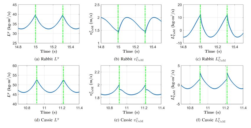
Figure 12.6: Angular momentum-based LIP-based controllers applied to two different robots: Rabbit and
Cassie. Rabbit is a 2D biped with five links, four actuated joints. Cassie is a 3D biped robot with 7 degrees
of freedom on each leg and five of them are actuated by motors. A floating-base model of Cassie has 20
degrees of freedom. The plot shows the comparison of L, Lcom , and vcom for Rabbit and Cassie. The results
of Rabbit are shown in the first row and the results of Cassie are shown in the second row. You can observe
that L (left column) is continuous at the impacts.12-8 Lecture 12: Locomotion Strategies of Boston Dynamics The references for this subsection are some of the talks given by Boston Dynamics’s employees [11, 12] (a disclaimer that the actual controllers behind the Boston Dynamics’ robots are veiled). The followings are the four layers of the overall framework of Spot, a quadrubed robot, from the lowest layer to the highest layer. 1. Servos and kinematics 2. Dynamics and balance via sequential composition [13] 3. Quadratic Program (QP)-based foot placement and obstacle avoidance 4. Navigation and autonomy Spot is stable and very robust. The technology behind it is the sequential composition of the funnels. The goal point of each local controller lies within the domain of attraction induced by the next local controller. Recently, this approach is also implemented on Cassie biped robot [14]. For the foot placement and the obstacle avoidance, it is likely that MPC that is linearized as a quadratic program is used at each time step, so that it can be solved in real-time. Atlas, a humanoid robot, has a very different framework from Spot. It uses momentum dynamics and kinematics, which has a trade-off between approximately capturing robot behavior and a light computation online. Its framework has four layers as bellow: 1. Offline trajectory optimization 2. Online model predictive control 3. Trajectory morphing 4. Behavior sequencing & blending First, in offline, a trajectory optimization using both moment dynamics and kinematics iteratively is done. This is a dense long-horizon optimization. When deploying it on the real robot, an online model predictive control will be executed which is a sparse short-horizon optimization. Both the offline and online optimiza- tions tackles the same problem so that the offline solution can be used for warm-starting the online MPC. This online MPC will also take care of the trajectory morphing if the environment have slight changes as well as behavior sequencing and blending. Discussion Prof. Tomlin: How is the robustness of such hierarchical methods compared to more intergrated planning and control methods? Zhongyu: The main concern of dividing decision variables into these different hierarchies is the computational cost. In the higher-level, reduced-order model is used for fast decision making and in the lower-level, a more sophisticated model can be used for low-level control. Prof. Sastry: There are different kinds of learning problems. For instance, learning strategies (for instance, jumping from one box to the next box) can use simplified models. There are also other problems like learning the dynamics model of foot placement and learning the terrain. What is interesting is that learning strategies and the dynamics model can happen offline, whereas adapting to new terrain can happen online (like in Prof. Malik’s work). Putting this all together, separating the time-scale adequately seems important like the sequential decomposition method depicts. Prof. Malik: Foot placement is one thing that learning can do a very good job. If there is a lot of obstacles in the environment. This is also related to Somil Bansal’s talk on learning-based visual navigation. This is
Lecture 12: Locomotion                                                                                   12-9

something that visual learning can do a very good job. Right now, model-based control for legged robots
is mainly about not falling off, and we know that this can be achieved without the vision because blind
people can walk well. When vision is more important is under trickier terrains like stepping stone scenario.
This has to be totally vision-driven. Vision will also provide forward anticipation (for instance, planning
multiple steps ahead). On the other hand, a critique to neural-network based approaches is that currently
there is no robustness analysis possible. It will be important to show capability of neural-network to achieve
high-performance dynamic motions. Why do specific gaits emerge from each type of animals? For instance,
walking and running emerge as human gaits whereas for horses, different gaits emerge such as galloping
and trotting. Such gaits should emerge, not programmed. Complex heavily-designed systems can often be
defeated by simpler systems.
Prof. Tomlin: Hybrid Zero Dynamics is a principled methodology, and has a control law that flattens out
everything into a simple low-dimensional manifold. This paradigm seems very principled and at the same
time, simple enough. What happens if you incorporate learning in this paradigm?

12.3      Learning-based Control for Locomotion
How to integrate learning in the control of legged robots?

   • There have been several attempts using supervised learning to design gaits that can be tracked by
     HZD-based controllers, as well as the gait transition policy. Prof. Grizzle’s group at University of
     Michigan have several works using this approach [15].

   • However, the most popular approach of integrating learning in the control of legged robots has been
     through reinforcement learning (RL). This started in the automated animation field of computer sci-
     ence. There have been works using imitation learning to obtain locomotion policies [16]. Also, some
     recent works use learning to learn the uncertainty in model-based controllers [17]. However, these
     works generally show results only in simulation, motivating the fact that it is necessary to develop
     good sim-to-real strategies to achieve real-world experimental results.
In the RL category, Prof. Marco Hutter’s group at ETH Zurich have presented some impressive results in
terms of robustness in experiments on their quadrupedal robot, ANYMAL [18]. Figure 12.7 shows their
control architecture. For training their policy, they use a teacher-student learning scheme. This consists
on having a teacher policy that is trained in simulation and has access to privileged information about the
environment, such as contact forces or terrain profile. Then, they train a student policy that does not have
access to the privileged information. This student policy takes a sequence of the history of the state of
the robot as input, feeding a TCN network. This TCN network is taught using imitation learning with
data aggregation (DAgger), trying to imitate the teacher policy. During training, they gradually increase
the difficulty (roughness) of the terrain by the use of curriculum learning. They deployed the robot in the
DARPA Subterranean Challenge and showed good performance.

Figure 12.7: Control architecture presented in [18]. A nominal foot trajectory generator produces a trajectory
for every foot. A neural network policy generates foot residuals and also the leg frequencies. Afterwards,
an inverse kinematics module and a joint-level PD controller are used. Note that no information from the
outside world is used.
12-10 Lecture 12: Locomotion
Figure 12.8: Control architecture presented in [20]. The RL policy directly outputs motor positions. The
input to the policy consists of four parts: i) the desired walking height, forward and turning velocities; ii)
the gait library reference motions; iii) a short history of the actions taken by the policy in the past; iv) a
short history of the states of the robot.
In a similar work [19], imitation learning is used to train locomotion policies for quadrupedal robots based
on the motions of real animals. Again, they use a latent space representation of the environmental dynamics.
Bipedal robots are, however, more challenging to control than the quadrupeds due to the fact that they are
statically unstable. In recent work [20], RL is used to control the Cassie bipedal robot. A single neural
network is used to let the robot track different velocities and walking heights. This RL framework builds on
top of the HZD controller that is normally used for Cassie. This HZD controller uses a gait library obtained
offline, from which a specific gait is tracked online using PD gait regulators and PD joint-level controllers.
There is a gain scheduling module for the PD controllers. It is clear that a lot of parameter tuning needs to
be carried out in order for this controller to work in experiments.
The RL framework of [20], that builds on top of the HZD controller that has just been explained, is presented
in Figure 12.8. PPO is used for the learning. Also, a curriculum is used during training in order to get
a faster learning progress. The resulting controller has been tested on both simulations and experiments,
showing robustness to obstacles, and recovery from severe disturbances.
This RL-based policy shows clear improvement over the baseline HZD controller. The feasible command set
(that includes desired walking height, forward and turning velocities) is four times bigger when using the RL
framework instead of the HZD controller. Basically, this means that the robot can walk faster, turn faster,
and walk higher and lower, by using RL than by using the HZD controller.
Remark: Model-based vs Learning-based Locomotion Control
Getting a model-based controller to work in simulation is very hard. Using learning, it becomes easier.
However, getting the learning-based controllers to work in experiments is harder than using model-based
controllers. This is because if something goes wrong in experiments using a model-based controller, there is
always some explanation to why this is happening, and we can improve the controller accordingly. However,
using a learning-based policy, if something goes wrong in experiments, there is no possible explanation to
that behavior, and a new policy needs to be trained.
12.4 Some Applications of Legged Robots
• Environment exploration for disaster response. Legged robots can traverse harsh terrains and cluttered
environments.
• Human-robot dynamic interaction. Recent work explores how to make Cassie express emotive behaviors
[21]. Also, there is a recent work on how to use quadrupedal robots to guide a blindfolded person using
a leash [22].
• A challenging problem that will be explored in the future is how to achieve bipedal robot running.
Learning-based methods seem very promising for this.Lecture 12: Locomotion 12-11
References
[1] R. Hartley, M. Ghaffari, R. M. Eustice, and J. W. Grizzle, “Contact-aided invariant extended kalman
filtering for robot state estimation,” The International Journal of Robotics Research, vol. 39, no. 4, pp.
402–430, 2020.
[2] R. Hartley, M. G. Jadidi, L. Gan, J. Huang, J. W. Grizzle, and R. M. Eustice, “Hybrid contact preinte-
gration for visual-inertial-contact state estimation using factor graphs,” in 2018 IEEE/RSJ International
Conference on Intelligent Robots and Systems (IROS), 2018, pp. 3783–3790.
[3] N. Aghannan and P. Rouchon, “On invariant asymptotic observers,” in Proceedings of the 41st IEEE
Conference on Decision and Control, 2002., vol. 2, 2002, pp. 1479–1484 vol.2.
[4] S. Bonnabel, P. Martin, and P. Rouchon, “Non-linear symmetry-preserving observers on lie groups,”
IEEE Transactions on Automatic Control, vol. 54, no. 7, pp. 1709–1713, 2009.
[5] J. Di Carlo, P. M. Wensing, B. Katz, G. Bledt, and S. Kim, “Dynamic locomotion in the mit cheetah 3
through convex model-predictive control,” in 2018 IEEE/RSJ International Conference on Intelligent
Robots and Systems (IROS), 2018, pp. 1–9.
[6] M. Chignoli and P. M. Wensing, “Variational-based optimal control of underactuated balancing for
dynamic quadrupeds,” IEEE Access, vol. 8, pp. 49 785–49 797, 2020.
[7] X. Xiong and A. Ames, “3d underactuated bipedal walking via h-lip based gait synthesis and stepping
stabilization,” arXiv preprint arXiv:2101.09588, 2021.
[8] Y. Gong and J. Grizzle, “Angular momentum about the contact point for control of bipedal locomotion:
Validation in a lip-based controller,” arXiv preprint arXiv:2008.10763, 2020.
[9] Y. Gong, R. Hartley, X. Da, A. Hereid, O. Harib, J. Huang, and J. Grizzle, “Feedback control of a
cassie bipedal robot: Walking, standing, and riding a segway,” in 2019 American Control Conference
(ACC), 2019, pp. 4559–4566.
[10] E. Daneshmand, M. Khadiv, F. Grimminger, and L. Righetti, “Variable horizon mpc with swing foot
dynamics for bipedal walking control,” IEEE Robotics and Automation Letters, vol. 6, no. 2, pp. 2349–
2356, 2021.
[11] M. Raibert, “Building dynamic robots, boston dynamics,” Turing Lecture. [Online]. Available:
https://youtu.be/yLtdzJ6mVMk
[12] S. Kuindersma, “Recent progress on atlas, the world’s most dynamic humanoid robot,” Robotics
Today. [Online]. Available: https://youtu.be/EGABAx52GKI
[13] R. R. Burridge, A. A. Rizzi, and D. E. Koditschek, “Sequential composition of dynamically dexterous
robot behaviors,” The International Journal of Robotics Research, vol. 18, no. 6, pp. 534–555, 1999.
[Online]. Available: https://doi.org/10.1177/02783649922066385
[14] Y. Zhao, “Robust planning and decision-making for safe legged locomotion,” USC Viterbi CPS
Webinar. [Online]. Available: https://youtu.be/ayD1m6wK2iY
[15] X. Da, R. Hartley, and J. W. Grizzle, “Supervised learning for stabilizing underactuated bipedal robot
locomotion, with outdoor experiments on the wave field,” in 2017 IEEE International Conference on
Robotics and Automation (ICRA), 2017, pp. 3476–3483.
[16] X. B. Peng, P. Abbeel, S. Levine, and M. van de Panne, “Deepmimic: Example-guided deep reinforce-
ment learning of physics-based character skills,” ACM Transactions on Graphics (TOG), vol. 37, no. 4,
pp. 1–14, 2018.12-12 Lecture 12: Locomotion
[17] J. Choi, F. Castaneda, C. J. Tomlin, and K. Sreenath, “Reinforcement learning for safety-critical control
under model uncertainty, using control lyapunov functions and control barrier functions,” arXiv preprint
arXiv:2004.07584, 2020.
[18] J. Lee, J. Hwangbo, L. Wellhausen, V. Koltun, and M. Hutter, “Learning quadrupedal
locomotion over challenging terrain,” Science Robotics, vol. 5, no. 47, 2020. [Online]. Available:
https://robotics.sciencemag.org/content/5/47/eabc5986
[19] X. B. Peng, E. Coumans, T. Zhang, T.-W. Lee, J. Tan, and S. Levine, “Learning agile robotic locomotion
skills by imitating animals,” arXiv preprint arXiv:2004.00784, 2020.
[20] Z. Li, X. Cheng, X. B. Peng, P. Abbeel, S. Levine, G. Berseth, and K. Sreenath, “Reinforcement learning
for robust parameterized locomotion control of bipedal robots,” arXiv preprint arXiv:2103.14295, 2021.
[21] Z. Li, C. Cummings, and K. Sreenath, “Animated cassie: A dynamic relatable robotic character,” arXiv
preprint arXiv:2009.02846, 2020.
[22] A. Xiao, W. Tong, L. Yang, J. Zeng, Z. Li, and K. Sreenath, “Robotic guide dog: Leading a human
with leash-guided hybrid physical interaction,” arXiv preprint arXiv:2103.14300, 2021.You can also read