Impact of user density increase on 802.11ax based Network Optimization

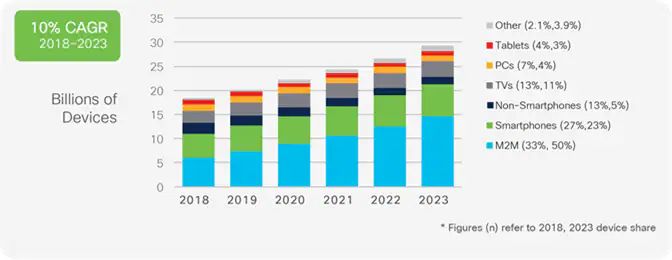
Impact of user density increase on 802.11ax based Network Optimization
SIETZE VAN DER VINNE, University of Twente, The Netherlands

The number of networked devices is increasing rapidly with numbers reach-
ing 29.3 billion by 2023, up from 18.4 billion in 2018. This increasing user
density requires new technologies to provide reliable connectivity. 5G and
IEEE 802.11ax are among these technologies. Deployment of Artificial Intel-
ligence (AI) in wireless networks has been proven useful in optimizing dense
networks, however optimization frameworks proposed in literature lack
analysis of user density variation over optimization time and performance
improvements. In this paper, Contention Window (CW) optimization in
802.11ax networks has been analysed because it has been shown to improve
network performance significantly. The analysis shows that throughput
varies from 33.9 Mbits/s with 5 users in the network to 32.7 Mbit/s with 50 Fig. 1. Global device and connection growth. Source: [5]
users in the network while delay and jitter variations remain within 45 and
14 milliseconds, respectively. The analysis reveals CW optimization can help
improve performance in dense networks and this analysis can help network
 researchers are trying to find ways for Access Points (AP) and edge
administrators to deploy cost-optimized networks.
 devices to work more and more efficient. Internet standard IEEE
Additional Key Words and Phrases: Deep Reinforcement Learning, IEEE 802.11ax is a result of such research and released in 2020. This new
802.11ax, Throughput, Wireless LAN, Contention Window, DRL based Opti- standard is more efficient than its predecessors, especially when it
mizations, User density in WLANs comes to higher user density. It employs OFDMA to support high
 user density however, it still follows the Contention-based channel
1 INTRODUCTION access mechanism.
As can be seen from figure 1, the number of connected devices grows When user density grows channel access becomes very complex
by billions every year [5]. One of the biggest growing categories and induces a lot of collisions. To get access to the channel the
is Machine-to-Machine (also called IoT) devices. It is forecasted station checks if the channel is idle and then transmits its data
that 50 per cent of total connected devices will be M2M devices frame. The station waits for an acknowledgement to see if there
by the end of 2023, of which around half is wireless. That is why was no collision before it proceeds with the next frame. If there
 was no acknowledgement there was most likely a collision and it
TScIT 37, July 8, 2022, Enschede, The Netherlands waits a random number of time slots between 0 and the Contention
© 2022 University of Twente, Faculty of Electrical Engineering, Mathematics and
Computer Science.
 Window (CW) to avoid another collision. When the channel does
Permission to make digital or hard copies of all or part of this work for personal or not get an acknowledgement it doubles the CW and this continues
classroom use is granted without fee provided that copies are not made or distributed until the station gets an acknowledgement and it will then send the
for profit or commercial advantage and that copies bear this notice and the full citation
on the first page. To copy otherwise, or republish, to post on servers or to redistribute rest of the frames. This way of choosing CW can be very inefficient
to lists, requires prior specific permission and/or a fee. in networks with a high user density and setting the right CW is

 1

TScIT 37, July 8, 2022, Enschede, The Netherlands Sietze van der Vinne

very important to the performance of a WiFi network [3]. That is Delays, Jitter and CW values are monitored and collected for the
why researchers are trying to find techniques to optimize the CW DRL algorithm to perform CW optimization.
value.
 Optimization of CW can be efficiently done with the help of 3.1 Ns-3 and Ns3-gym
Machine learning-based algorithms like DRL [11] or supervised For the simulations, a combination of Ns-3 and ns3-gym is used.
learning (SL) [8] and throughput improvements have been achieved Ns-3 is an open-source network simulator developed in C++ using
compared to conventional optimization techniques. Now with the object orienting programming model and is widely used in network
increase of devices, it is important to understand all the conse- research. Ns-3 can simulate the latest 802.11ax network models
quences of user density increase in such optimized networks like and allows sophisticated tracing and monitoring of the network.
latency or the convergence speed of the DRL. This can help network Ns3-gym uses the OpenAI Gym[2] RL toolkit. Given numerical data
administrators decide on the employment of CW optimization solu- of observations, actions and rewards OpenAI Gym can train a RL
tions and design more robust and efficient networks while reducing agent. Ns3-gym is a framework that uses this toolkit specifically for
infrastructure costs. RL research in networking.
 The objective of this research is to find out how user increase af- In this paper, an open-source framework [11] has been used which
fects CW optimization time and overall network performance. This already has a DRL algorithm for CW optimization.
analysis will help design WiFi networks keeping in view anticipated
user density. The analysis can also be used to design cost-effective 3.2 Data
networks with minimal infrastructure to support a given user den- In these simulations, user density has been increased and the effects
sity. In order to perform this analysis, network simulations were on DRL and certain aspects of the network have been analyzed.
carried out in NS3 with the CW optimization framework used in All simulations have been run twice, once with CW optimization
[11]. and once with standard 802.11ax. Later the results are analyzed and
 compared for improvement. So in this quantitative research, the
2 RELATED WORK following data on networks with varying number of stations from
A lot of research has been done on network optimization with ML. 5,10,....,N has been collected:
The articles in the introduction [11](using ML and neural networks) • Optimization time (the time it takes for the DRL algorithm to
and [8](using ML without neural networks) are examples of CW learn the optimal CW value).
optimization. But there are other parameters that can be optimized • Throughput of the network (successfully transferred data in
using ML. Like frame length optimization using Supervised Learn- Mbits/second).
ing [7], they were able to achieve an improvement of 18.36% in • Latency (Time it takes for a packet to be received).
throughput by optimizing the length of the packet frames using • Jitter (delay variation in seconds).
Supervised Learning. Applying RL to optimize the data transmis- The gathered data will be presented in graphs. From these graphs,
sion rate [4] is another example, here the data sending rates of conclusions will be drawn and a real-life environment will be sketched
nodes is controlled with a DRL agent and higher throughput was to see if network costs can be reduced.
achieved. Or this research [1], where DRL is used to solve time and
resource allocation problems in OFDMA wireless networks. Higher 3.3 Network and study model
throughput was achieved here as well. ML research in other wireless The simulated network consists of one AP and varying number of
networks like Long-Term Evolution (LTE) has also been done [9], stations from 5,10,....,N. These stations will constantly send UDP
this research also achieved higher throughput. packets with a fixed size of 1500B to the AP. The CW-value is calcu-
 Some of these papers have an analysis of how varying user density lated with the DRL algorithm and then broadcasted to all stations
affects throughput, but other effects are left out. This paper will in the neighbourhood. After receiving these broadcasts all stations
show how CW optimization in 802.11ax networks ... update their CW accordingly. The network topology is shown in fig-
 ure 2 and while network parameters used in simulations are given
 • affects jitter with varying user density.
 in Table 1. Around 20% of the connected stations are stationary,
 • affects delay with varying user density.
 and the rest of the stations are mobile. All stations are connected
 • affects throughput with varying user density.
 wirelessly.
 • can best be deployed.
 • can reduce network costs. 3.4 DRL Framework
 The DRL framework used in [11] has been used in this study. In RL
3 METHODOLOGY there is an agent who can perform certain actions in an environment.
To study the effects of increasing user density on CW optimization In this framework, the RL agent is centralized at the Access Point
networks simulations have been used. IOT sensors and M2M devices (AP). The environment is the wireless network and the action the
are represented as nodes with varying traffic requirements. Traffic agent can take is to broadcast a certain CW.
generation is done from nodes towards AP and from AP towards The goal of the agent is to optimize its parameters, in this case, the
nodes. Parameters like bandwidth, packet size and CW are set up CW. The agent learns how to reach this goal by means of rewards and
as per IEEE 802.11ax standard. Network statistics like throughput, punishments. Throughput is a good measure of the performance of

 2

Impact of user density increase on 802.11ax based Network Optimization TABLE
 TScIT 37, July 8,I2022, Enschede, The Netherlands
 CCOD’ S DRL SETTINGS
 # AP 1
ast # Stations 5 up to N
W IEEE 802.11ax Parameter Value
 Modulation 1024-QAM
 Channel width 20 MHz Interaction period 10 ms
 Packet protocol UDP
 Sent frames
 Packet size 1500B History length ℎ 300
 Table 1. Network settings DQN’s learning rate 4 × 10−4
 DDPG’s actor learning rate 4 × 10−4
 DDPG’s critic learning rate 4 × 10−3
 Batch size 32
 Reward discount 0.7
 UDP UDP Replay buffer size 18,000
 Smart IoT Soft update coefficient 4 × 10−3
 Phone sensor
ce 64 CW-value
 CW-value Table 2. DRL settings

 CW 42
 UDP UDP
 Wireless Access
 40
 Network throughput [Mb/s]

 CW-value CW-value algorithm to work optimally. They have been chosen like this by
 Point
s transmit data to the AP) and process means of trial and error after many simulations.
 38 To help the agent explore more possible actions a certain random-
 andard deviation).
 ization factor is added to the decision of the agent. This so-called
 36 noise makes sure the agent does not get stuck on the first decision
 Laptop PC it gets rewarded on. The noise decreases every step. When the noise
 ON M ODEL is zero the agent will always make the best-known decision.
 Improvement
 34 over 802.11
 ns3-gym [20], which is a 4 RESULTS
 32 Jitter (variation in time delay), Throughput (received bits by the AP
 (a network simulator) with per second) and Delay (the time it takes for a packet to reach its
 Standard 802.11
nalysis).Fig.The neural
 2. Network networks
 topology: stations
 30
 sent UDP packets, AP broadcasts CW. destination) are measured because it gives a good representation of
 Look-upof table
 the performance the network. DRL optimization time has been
emented in Pytorch and Ten- measured to give an insight on how long it would take before the
 CCOD w/ DQN
 28 network can perform optimally. In the simulations all devices stay
strate independence of agent
 the network and is therefore used as a reward factor. The algorithm
 works in steps, in every step, a CW is chosen and the throughput is
 CCOD w/ DDPG
 connected and are constantly sending data, this is different from real-
 world networks. This means that the results may also be different
 measured. If the throughput has increased or decreased since 26the from real-world networks. A few extra connected devices that send
 0
 last step the agent is rewarded or punished respectively. The frame- 10data would however
 little to no 20 have comparable
 50 30 effects on 40 standard
 e topology of Fig. 1 and the
 work’s algorithm uses Neural Networks to learn from its experience
 Number of stations
 802.11ax as to an optimized network. This is because they would
 and determine the CW, which makes this a DRL algorithm. The rarely request channel access.
dio channels, IEEE 802.11ax,
 framework has two options for the algorithms: discrete (DQN) and
 continuous (DDPG). In this paper, only the DDPG method is used, Fig. 2. Network throughput for the static topology.
ng scheme (1024-QAM with a
 since the research from this paper[11] shows that this method has 4.1 Throughput
 higher throughput than the discrete method. The settings of the DRL As you can see figure 3 shows the network throughput for three
 smissions, a 20 MHz channel,
 algorithm are shown in table 2 [11]. DDPG has two neural networks, different situations. Throughput (no optimization), which is the
d constant bit-rate UDP uplink networks was determined in the same way as the
 one for the actor who gives an action directly from a state and one average throughput of the standard 802.11ax. Then Throughput
 for the critic who takes the state and action as input and outputs (total), which is the average throughput during and after training.
 B packets and equal offered hyperparameters. Using a recurrent layer with a wide h
 the expected reward. Both the critic and the actor network had the And Throughput (after training) which is the average throughput
 following layers structure: 8 × 128 × 64. The hyper-parameters in after the training is done. At 50 stations the throughput is 23% higher
 network. Also, we assumed window allowed the algorithms to take previous observ
 table 2 and the network configuration are all important for the DRL in the network with optimization after training.

 sfer of state information to into account.
 3
 The preprocessing window length was se
 es of and are known with a stride of ℎ4 , where ℎ is the history length.
e immediate setting of Randomness was incorporated into both agent behavi
axing the former assumption network simulation. Each experiment was run for 15 r

TScIT 37, July 8, 2022, Enschede, The Netherlands Sietze van der Vinne

 25

 20
 39

 Jitter (ms)
 15
 37
 10
 35
 Throughput [Mb/s]

 5
 33
 0
 6 10 20 30 40 50
 31
 Number of stations
 29
 Average Jitter (ms) Average Jitter (no optmization)(ms)

 27

 Fig. 5. Jitter in milliseconds
 25
 5 10 15 20 25 30 35 40 50

 Number of stations

 Throughput (total) 60
 Througput (after training) 50
 Throughput (No Optimization) 40
 Delay (ms)
 30

 Fig. 3. Throughput in Mb/s 20
 10
 0
 6 10 20 30 40 50
 Number of stations
 200
 180
 End-to-end Delay (ms) End-to-end Delay (no optimization)(ms)

 160
 optimization time (m)

 140
 120
 Fig. 6. Delay in milliseconds
 100
 80
 4.3 Jitter and Delay
 60
 40 And figure 5 shows the average jitter in he network in milliseconds.
 20 The jitter is approximately the same for 6 up to 40 stations. At 50
 0 stations the optimized network has 45% less jitter.
 0 10 20 30 40 50 60
 Lastly, figure 6 shows the average of all end-to-end delays of the
 Number of Stations
 received packets. As with jitter the delay is approximately the same
 for 6 up to 40 stations. At 50 stations the delay is 30% less for the
 optimized network.
 Fig. 4. optimization time in minutes
 5 ANALYSIS AND DISCUSSION
 In this section, an example will be given of how a network admin-
 istrator can reduce the cost of a network using CW optimization.
4.2 Optimization Time An example of a network with a lot of wirelessly connected sensors
Figure 4 shows how long it takes for the DRL agent to optimize the and devices is the network of a hospital.
CW in minutes. The training was done with a i7-9750H CPU at 2.60
GHz. The training time increases from 25 minutes for 5 stations to 5.1 throughput
173 minutes for 50 stations. These optimization times are high, but Table 3 shows some data rates of typical devices in such a network
once an agent is trained it does not need to be retrained until the according to [10]. Now as an example suppose a hospital floor uses 5
network topology changes a lot. This is because the neural network EMGs, 10 digital audio stethoscopes and 10 ECGs for their patients.
is already optimal for that network topology. This would need only 4.35 Mb/s of throughput. If 5 physicians are

 4

Impact of user density increase on 802.11ax based Network Optimization TScIT 37, July 8, 2022, Enschede, The Netherlands

 Digital device Data rate 6 CONCLUSION
 Digital audio stethoscope (heart sound) ∼120kbps The IEEE 802.11ax network standard was designed to cope with
 Electromyogram EMG ∼600kbps high-density networks. From this research, it may be concluded that
 Electrocardiogram ECG ∼15kbps this network standard can be improved when it comes to through-
 Medical video for teleconsultation put, delay and jitter. This can be done with the help of Contention
 ∼1.544Mb/s Window optimization. Because of this improvement, the cost of
 (e.g.,ophthalmoscope, proctoscope, etc.)
 Voice/video/chat communication of high-density networks can be reduced by 33%.
 384kbps to 1.544Mb/s
 commuting physicians
 Digital radiography (DICOM) 6MB (image size) REFERENCES
 [1] Ravikumar Balakrishnan, Kunal Sankhe, V. Srinivasa Somayazulu, Rath Van-
 Mammogram (DICOM) 24MB (image size) nithamby, and Jerry Sydir. 2019. Deep Reinforcement Learning Based Traffic- and
 Table 3. Typical medical data rates Channel-Aware OFDMA Resource Allocation. In 2019 IEEE Global Communica-
 tions Conference (GLOBECOM). 1–6. https://doi.org/10.1109/GLOBECOM38437.
 2019.9014270
 [2] Greg Brockman, Vicki Cheung, Ludwig Pettersson, Jonas Schneider, John Schul-
 man, Jie Tang, and Wojciech Zaremba. 2016. OpenAI Gym. CoRR abs/1606.01540
 (2016). arXiv:1606.01540 http://arxiv.org/abs/1606.01540
 [3] Yunli Chen and Dharma Agrawal. 2004. Effect of Contention Window on the
having a teleconsultation and 5 communicating over video, this performance of IEEE 802.11 WLANs. (01 2004).
would need 15.44 Mb/s of throughput. Now suppose one of those [4] Soohyun Cho. 2020. Rate Adaptation with Q-Learning in CSMA/CA Wireless
physicians wants to download a digital radiography (6 MB = 48 Networks. Journal of Information Processing Systems 16 (10 2020), 1048–1063.
 https://doi.org/10.3745/JIPS.03.0148
Mbits) at the same time within 4 seconds, this would need another [5] Cisco. 2018, updated 2020. Cisco Annual Internet Report (2018–2023) White Paper.
12 Mb/s of throughput. In total 31.79 Mb/s of throughput is needed Technical Report. Cisco.
 [6] Giulia Cisotto, Edoardo Casarin, and Stefano Tomasin. 2020. Requirements and
for 30 devices. From 3 we can conclude that this would need either Enablers of Advanced Healthcare Services over Future Cellular Systems. IEEE
2 APs without CW optimization or one AP with CW optimization. Communications Magazine 58, 3 (mar 2020), 76–81. https://doi.org/10.1109/mcom.
 If instead of two physicians having a teleconsultation there would 001.1900349
 [7] Estefanía Coronado, Abin Thomas, and Roberto Riggio. 2020. Adaptive ML-Based
be 22 extra ECGs, then the required throughput would be 30.601 Frame Length Optimisation in Enterprise SD-WLANs. J. Netw. Syst. Manage. 28, 4
Mb/s. This would be even less throughput, but because the user (oct 2020), 850–881. https://doi.org/10.1007/s10922-020-09527-y
density now has increased to 50 stations an AP without CW opti- [8] Yalda Edalat and Katia Obraczka. 2019. Dynamically Tuning IEEE 802.11’s Con-
 tention Window Using Machine Learning. In Proceedings of the 22nd International
mization would have even more problems handling the data. ACM Conference on Modeling, Analysis and Simulation of Wireless and Mobile Sys-
 Given that the AP has the same bandwidth (maximum rate of tems (Miami Beach, FL, USA) (MSWIM ’19). Association for Computing Machinery,
 New York, NY, USA, 19–26. https://doi.org/10.1145/3345768.3355920
data transfer) as the AP from the simulation. This is of course a very [9] Ahmed M. El-Shal, Badiaa Gabr, Laila H. Afify, Amr El-Sherif, Karim G. Seddik,
specific example but it does show how, if the CW optimization was and Mustafa Elattar. 2021. Machine Learning-based Module for Monitoring
free, the cost of a network can be halved. LTE/WiFi Coexistence Networks Dynamics. In 2021 IEEE International Conference
 on Communications Workshops (ICC Workshops). 1–6. https://doi.org/10.1109/
 ICCWorkshops50388.2021.9473865
5.2 Jitter and delay [10] Dimitris Komnakos, Demosthenes Vouyioukas, Ilias Maglogiannis, and Philip
 Constantinou. 2008. Performance evaluation of an enhanced uplink 3.5G system
In this article [6], requirements for future healthcare applications for mobile healthcare applications. Int. J. Telemed. Appl. 2008 (Dec. 2008), 417870.
are given. Examples are "remote pervasive monitoring" and "Mobile- [11] Witold Wydmański and Szymon Szott. 2021. Contention Window Optimization in
 IEEE 802.11ax Networks with Deep Reinforcement Learning. In 2021 IEEE Wireless
health wearables" which both allow for a maximum jitter of 25 Communications and Networking Conference (WCNC). 1–6. https://doi.org/10.
ms. The average jitter of an AP without CW optimization with 50 1109/WCNC49053.2021.9417575
connected stations is 20.1 ms, but in some connections, jitter did [12] Song Xu, Manuela Perez, Kun Yang, Cyril Perrenot, Jacques Felblinger, and Jacques
 Hubert. 2014. Determination of the latency effects on surgical performance and
exceed 25 ms. For the optimized network, this was not the case the acceptable latency levels in telesurgery using the dV-Trainer(®) simulator.
and the average jitter was 45% less. For 40 stations or less CW Surg. Endosc. 28, 9 (Sept. 2014), 2569–2576.
optimization can not make a difference, but when the user density
grows and too much jitter is becoming a problem, CW optimization
can be considered as a solution.
 The same goes for delay (30% improvement at 50 stations) which
could be of importance when it comes to telesurgery [12].

5.3 Cost reduction
From the example, it can be concluded that the number of APs can
be halved in some situations. Assume a network administrator has
to provide the wireless network of a hospital with three floors. He
could either choose two standard 802.11ax routers per floor which
are around €60 or one with a bit more computing power to better
handle the DRL training which would be around €80 at the time of
writing. For three floors this would give a cost reduction of €120
which is 33%

 5