Information and Market Efficiency: Evidence From the Major League Baseball Betting Market

Information and Market Efficiency:
 Evidence From the Major
 League Baseball Betting Market
 The Harvard community has made this
 article openly available. Please share how
 this access benefits you. Your story matters

Citation Bouchard, Matthew. 2019. Information and Market Efficiency:
 Evidence From the Major League Baseball Betting Market.
 Bachelor's thesis, Harvard College.

Citable link https://nrs.harvard.edu/URN-3:HUL.INSTREPOS:37364609

Terms of Use This article was downloaded from Harvard University’s DASH
 repository, and is made available under the terms and conditions
 applicable to Other Posted Material, as set forth at http://
 nrs.harvard.edu/urn-3:HUL.InstRepos:dash.current.terms-of-
 use#LAA

Information and Market Efficiency: Evidence from the Major League
 Baseball Betting Market

 A thesis presented

 by

 Matthew Bouchard

 To

 Applied Mathematics

 In partial fulfillment of the honors requirement

 For the degree of

 Bachelor of Arts

 Harvard College

 Cambridge, Massachusetts

 March 29, 2019

Abstract

 Evaluating market response to information is difficult in traditional financial

markets due to their complex pricing problem. Sports betting markets greatly simplify this

process. Therefore, I use moneyline data from over 88,000 Major League Baseball (MLB)

games to explore the evolution of efficiency in the MLB betting market from 1977 to 2018,

analyzing the manner in which it assimilates information. By comparing forecasting

accuracy across years, I find that improving precision is driving a convergence between

forecasts and outcomes over time, spurred specifically by changes occurring from the late

1990s to early 2000s. This period corresponds to improvements in information quality,

quantity, and accessibility in the market. I then show that information assimilation within

each season, through the incorporation of current-season performance, leads to an increase

in accuracy. By comparing daily opening and closing lines, I find that larger relative line

movements are on average less accurate, suggesting exaggerated market reactions to new

information and highlighting the importance of information processing time on efficiency.

In addition, I offer suggestive evidence of informed bettor presence but am unable to fully

disentangle the relationships between betting volume, better composition, and accuracy.

 ii

Acknowledgements

 I would like to express my sincere gratitude to all those who helped and supported

me throughout this research process. I am indebted to Dr. Judd Cramer and Dr. Andrés

Maggi, who have been tremendous advisers and mentors, providing invaluable insight and

guidance. Without them, this thesis could not have been possible. I thank Professors Matt

Ryan, Andrew Weinbach, and Bill Dare, along with my roommate Niklas Boström, for

their help acquiring data. I very much appreciate Ryan Davis and Rana Bansal for reading

drafts and suggesting helpful edits. I am fortunate to have the support of friends like them,

whom I can always rely on. Finally, I thank my family – Mom, Dad, Luke, and Bella – for

their endless love and support in anything that I do.

 iii

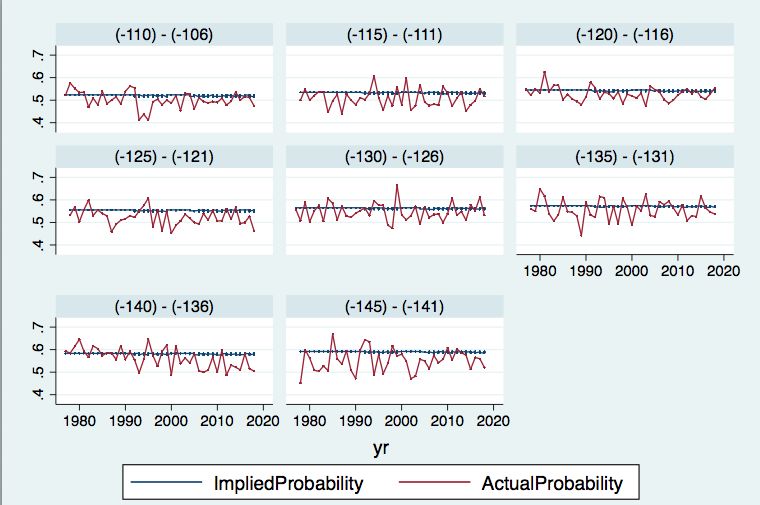
Table of Contents
I. Introduction ........................................................................................................ 5
II. Literature Review ............................................................................................ 8
III. Data................................................................................................................12
IV. Methodology ...................................................................................................14
 Overall Market Dynamics................................................................................................. 15
 Information Assimilation .................................................................................................. 18
 Line Movements................................................................................................................ 21
V. Results................................................................................................................22
 Overall Market Dynamics................................................................................................. 22
 Information Assimilation: Learning Rates Within Season ............................................... 24
 Information Assimilation: Learning Rates Over Time ..................................................... 25
 Information Assimilation: Impact of the NFL Season by Day of the Week...................... 25
 Line Movements................................................................................................................ 27
VI. Discussion ......................................................................................................28
VII. Conclusion .....................................................................................................32
References .................................................................................................................34
Tables and Figures ....................................................................................................38
Appendix....................................................................................................................54
 A.1 Terminology ............................................................................................................... 54
 A.2 Data ............................................................................................................................ 55
 I. Adjustments ............................................................................................................ 55
 II. Comparison of Data Sources ................................................................................. 56
 A.3 Test of Line Group Efficiency .................................................................................... 57
 A.4 Line Movement Deciles .............................................................................................. 59
 A.5 Line Movement Sensitivity Check .............................................................................. 60

 iv

I. Introduction
 As proposed by Fama (1970), the efficient market hypothesis (EMH) states that the

price of an asset fully reflects all available information related to its intrinsic value. This

implies that participants are not able to use publicly available information to consistently

generate excess returns relative to the market. While Fama (1970) finds that the EMH

performs exceptionally well in the vast majority of securities markets, research in

subsequent decades reveals anomalous, profitable trading strategies and criticizes the

assumption of market efficiency (Rozeff and Kinney 1976, French 1980, Banz 1981).

However, following the publication of such strategies like the January or Small Firm

Effects, their profitability gradually vanishes from the market, arbitraged away by informed

investors (Horowitz et al. 2000, Malkiel 2003, Szakmary and Keifer 2004). These findings 1

highlight a fundamental assumption of efficient markets – that prices not only reflect

existing information but also respond to new information. The new information of

potentially profitable trading strategies diffuses throughout the market, and prices adjust to

eliminate them. As a result, there is considerable economic interest to better understand

how markets incorporate information. In this paper, I use the Major League Baseball

(MLB) betting market as a testing grounds to study the impact of information, in regard to

its assimilation, quality, and quantity, on efficiency.

 Study of the MLB betting market has distinct advantages, especially relative to

capital markets. Not only does it represent a simplified financial market with a vastly

simplified pricing problem, but also the true, underlying value of the asset (the bet) is

1
 The January Effect is the tendency for the price of stocks to rise more in January than in other months, while
the Small Firm Effect is the tendency for smaller firms to have higher risk adjusted returns, on average, than
large firms (Rozeff and Kinney 1976, Banz 1981).

 5

known with certainty after the conclusion of a game (Sauer 1998, Levitt 2004).

Furthermore, it is a major source of economic activity, generating an annual $55 billion in

both legal and illegal bets (Purdum 2016). Although half the size of the NFL betting

market, the MLB betting market has a vast edge in regard to its volume of events. Whereas

the NFL regular season consists of only 256 games, the MLB regular season has a total of

2,430 games, yielding far larger sample sizes for analysis. The final research advantage of

the MLB betting market concerns its relationship with information – more so than any

other sport, MLB has seen an explosion in the amount and quality of information available

to it. Online databases contain statistics going back to the 1800s, and there is even a

dedicated field of research, known as sabermetrics, that empirically analyzes statistics to

predict performance. Newer developments like Statcast quantify more aspects of the game

than ever before, enabling novel insights and analyses that are publicly available. 2

 In this context, I exploit a dataset of over 88,000 MLB games’ gambling lines to

study the evolution of the baseball betting market’s efficiency from 1977 to 2018,

particularly as it relates to information responses. I first compare the market’s forecasts

against actual outcomes across years, using a series of weighted least squares regressions

in order to test their accuracy and precision and identify periods of substantial shifts in

market dynamics. I proceed to adopt a more granular view, looking at within-season

dynamics of information assimilation by examining forecasting errors on a weekly basis.

Lastly, I consider information assimilation on an even more granular scale, estimating the

information content of daily line changes by studying their impact on prediction error.

2
 Statcast, released in 2015, records vast amounts of data related to every aspect of baseball performance,
including pitching, hitting, fielding, and baserunning, for every pitch and play of every game. The public can
access all of these data.

 6

I find that the dominant market dynamic is increasing forecast precision, enabling

consistent prediction accuracy. I show that this trend is driven by changes in the late 1990s

to early 2000s, and I proceed to offer plausible explanations in terms of both the quality

and quantity of information available to the market. I also find that market forecasting

accuracy significantly improves over the course of a season - out of 80 similarly priced

games, the market correctly predicts game outcomes toward the end of the season on

average 4.29 more times compared to the start of the season. The beginning of the National

Football League (NFL) season alters this trend and decreases overall accuracy. The market

correctly predicts the favorite 2.66 more times on average in an 80-game week if the week

occurs just prior to the start of the NFL season compared to after. However, the rate at

which this information assimilation occurs has not accelerated over time. Finally, I find

that, on average, larger line movements lead to larger prediction errors: a 1% increase in

magnitude of the percent change of a line leads to incorrectly predicting the favorite 2.53

more times on average out of 1000 games. While the results suggest that oddsmakers bias

their lines and informed bettors take advantage of these biases, I am unable to arrive at

conclusive results.

 The remainder of the paper proceeds as follows. Section II discusses the related

literature, while Section III presents the data. Section IV describes the empirical strategy.

Sections V and VI report the results and their implications, respectively. Section VII

concludes.

 7

II. Literature Review
 Information is crucial for market functionality. The EMH assumes that prices

reflect all current information, but prices also must respond to incorporate the release of

new information. Several studies analyze this concept in the stock market, demonstrating

that prices respond in the expected direction after news events such as stock splits, though

the speed of response varies (Fama et al. 1969, De Bondt and Thaler 1995, Campbell et al.

1997). However, it is the study of commodity markets that provides the most substantive

analyses showing the impact of information, particularly in terms of its accessibility, on

market functionality. Jensen (2007) finds that the introduction of mobile phones to the

Indian fisheries sector lowered barriers to information access and led to near perfect market

efficiency, the elimination of waste, and overall consumer and producer welfare increases.

Studying the cotton industry, Steinwender (2018) demonstrates similar efficiency

improvements due to enhanced access to information. She finds that the introduction of the

telegraph reduced data acquisition barriers in the market to such an extent that there was a

welfare gain equivalent to the abolishment of a 6% ad valorem tariff. In addition, the grain

and livestock markets saw gains in efficiency with the release of information via production

and breeding reports (Larson 1960, Miller 1979).

 The literature has also studied the relationship between information and efficiency

through the lens of betting markets. The reason is that betting markets have the distinct

advantage that the true, underlying value of the asset (the bet) is much easier to ascertain.

In fact, it is known with certainty after the outcome of the event of interest. Overall, betting

markets represent simplified financial markets with a vastly simplified pricing problem

(Sauer 1998, Levitt 2004). Uncertainty initially surrounds the outcomes, and the large

 8

number of participants have extensive, yet incomplete, information that they utilize to

determine the market clearing prices, or odds. Additionally, while the market is primarily

composed of individual bettors and price information is widely available, there are

professional gamblers who try to exploit mispricing or sell their picks, much like traders

and fund managers (Avery and Chevalier 1999). Comparisons between ex ante measures,

represented by odds, and ex post measures, known with certainty after the gambling event

occurs, provide insight into efficiency and enable analysis of market response to

information.

 To date, the majority of economic research in wagering markets focuses on race-

track, American football, and European football betting due to the size and popularity of

these sports (Snyder 1978, Asch et al. 1984, Gray and Gray 1997, Gil and Levitt 2007).

For instance, over $100 billion is legally bet on horse-racing every year, while the

American and European football betting markets take in over $300 billion annually, legally

and illegally (Keogh and Rose 2013, Purdum 2016, The Jockey Club 2016). These markets

are major sources of economic activity, with large amounts of money at stake (Levitt 2004).

Although small relative to other sports, valued at approximately $55 billion, the use of the

MLB betting market provides distinct research advantages, particularly in regard to its

large volume of events (Purdum 2016). Additionally, the study of the MLB betting market

provides nuance to existing NFL literature, especially in terms of the rate and effectiveness

of information incorporation since the time frame for market adjustments is very different.

Specifically, NFL opening odds come out one week before the game, whereas sportsbooks

release MLB opening odds the day before a game.

 9

Similar to other sports wagering research, prevailing literature related to the MLB

betting market has sought to test efficiency by searching for profitable betting strategies

that depend only on publicly available information at the time of the wager. The primary

focus of these studies is the closing line, which is the final value of the betting line at game

time and is regarded as the most accurate forecast of actual outcomes, as it reflects broader

market sentiments and contains more information (Gandar et al. 1988, Norheim 2017).

Woodland and Woodland (1994) find that the market is highly efficient in the sense that

objective win proportions correspond closely to subjective win probabilities (proxied by

closing lines), with a slight, but not exploitable, reverse favorite longshot bias. While later
 3

studies contest the existence of this bias, they nevertheless also find a high degree of market

efficiency (Gandar et al. 2002, Gandar and Zuber 2004, Paul et al. 2009, Ryan et al. 2012).

A limitation to these studies, however, is that they only consider efficiency cross-

sectionally, aggregating and evaluating prediction accuracy in one time period. In this

paper, I expand on this literature by examining the evolution of accuracy and efficiency in

the market across time. This enables a better understanding of how the market achieves

and maintains efficiency.

 Just as market efficiency can change across years, it can also change within a year.

This is especially relevant for sports betting markets, because as the season progresses team

performance reveals more and more information about underlying ability. Thus, individual

seasons are natural testing grounds for information incorporation: at the beginning of a

season, the market has limited information on a team’s true ability in the current season

3
 The favorite longshot bias is the tendency of bettors to overbet underdogs (longshots) and underbet
favorites. It is most common in horseracing, but the reverse of the bias has been documented in both the MLB
and NHL betting markets (Woodland and Woodland 2010).

 10

and relies on previous seasons’ information in its forecasts. As teams play more games,

current season information resolves the uncertainty concerning team performance, and as

a result, teams originally expected to perform poorly may become very successful or vice

versa. To the best of my knowledge, the only paper that explores this is Ryan et al. (2012),

which considers the timing within the season when bets are placed and finds that betting

on underdogs in April would have generated positive profits from 2001-2010. As with the

revelation of profitable trading strategies in the stock market, Ryan and Celestin (2018)

show that the profitability of this strategy disappears in the years following its release,

providing evidence of market response to information between seasons. Whereas these

studies only consider wagering strategies dependent on month of the season, I provide a

more nuanced view by studying the relationship between weekly prediction accuracy and

the number of games played in a season up to that week. This enables an estimate of the

rate at which the market incorporates in-season performance information and allows for a

comparison of these rates over time.

 The market can also incorporate information on a more granular scale – on a daily

basis for each game throughout the betting window. Bookmakers release their opening

lines up to a day before a game and can change the lines prior to game time due to betting

imbalances or the release of new information such as line-up changes, injury reports, or

weather forecasts. Most line movement research uses the NBA and NFL point spread
 4

markets as their testing grounds, finding that line changes carry information that improves

4
 See the Appendix for a slightly more in-depth description of lines, including definitions of the opening and
closing lines. By “line,” I am referring to the moneyline. I use the terms interchangeably throughout the
paper.

 11

accuracy and demonstrate the presence of informed, influential traders in the market

(Gandar et al. 1998, Gandar et al. 2000).

 On the other hand, analysis of MLB line movements is far more limited and

inconclusive, with only Paul and Weinbach (2008) examining line movements in the MLB

moneyline market. They find offshore sportsbooks to be highly efficient in the sense that

no profitable wagering strategies exist based off of general line movements. Interestingly,

they find betting against first movements to favorites is profitable for a smaller Las Vegas

sportsbook. However, they only use one year’s worth of data, so their conclusions might

not be externally valid. Rather than search for the existence of profitable wagering

strategies, I instead expand the MLB line movement literature by estimating the impact of

line movement direction and magnitude on prediction accuracy.

 III. Data
 This paper relies on two datasets - the first includes the closing moneylines and

outcomes for 88,306 Major League Baseball games from the years 1977 – 2018, and the

second consists of opening and closing moneylines and outcomes for 11,863 games from

the 2013 – 2018 seasons. The first dataset comes from two sources: the 1977 – 2000

seasons are from Computer Sports World (CSW) and the 2001 – 2018 seasons are from

Covers.com, an established offshore sports betting site.5 These sources are consistent with

prior literature (Woodland and Woodland 1994, Gandar et al. 2002, Paul and Weinbach

2008, Ryan et al. 2012). The combination of these two sources provides the largest MLB

moneyline dataset analyzed to date, spanning 42 seasons. While the use of two distinct

5
 Vegas Insider acquired Computer Sports World in the early 2000s and has since stopped providing archived
odds information. I am thankful to Professor Bill Dare at Oklahoma State University and Professor Andrew
Weinbach at Coastal Carolina University for providing me with their 1977 – 1999 CSW data.

 12

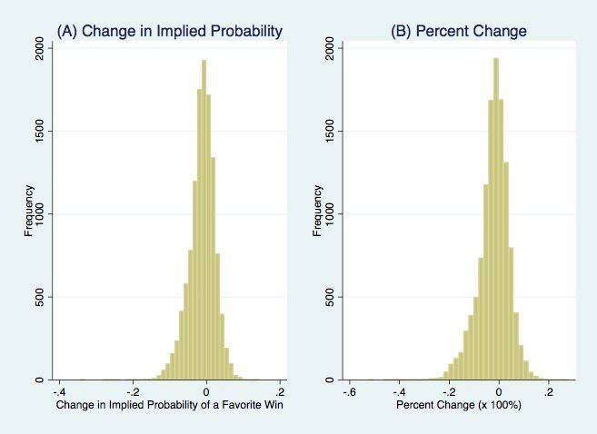
sources could confound results, since moneylines and forecasting ability vary by

oddsmakers, a comparison of two seasons of overlap reveals that the two sources are

extremely similar, with a mean difference between lines of just 0.03 points. Appendix A.2

contains further figures and descriptions that compare these two sources.

 Across all games in the aggregate dataset, there are 148 distinct lines represented.

Figure 1 displays their frequency of occurrence. The average implied probability of a

favorite win is 0.584, while the median value is 0.576. The 25th percentile is 0.545, the 75th

percentile is 0.615, and the standard deviation is 0.046. Overall, the minimum and

maximum implied probabilities of a favorite win are 0.515 and 0.737, corresponding to

moneylines of -106 and -280, respectively.

 In the sample, favorites have a 55.92% winning percentage. In over two-thirds of all

games, the favorite is the home team, with a winning percentage of 57.04%. In games

where the away team is the favorite, this value drops to 53.30%. Table 1 features an

additional breakdown of probabilities by month of the season, showing a general tendency

of the favorites to win more often as the season progresses. 6

 I use the second dataset to analyze line movements from the 2013 – 2018 seasons.

The data comes from donsbest.com, a gambling site that archives MLB game information

from 2013 onwards. While the closing line comes explicitly from the sportsbook Pinnacle,

the opening line source is not stated, but a comparison of a large number of the opening

lines shows that they do in fact come from Pinnacle as well. However, a main limitation to

using donsbest.com is the incompleteness of its data: 2,717 games had some form of

missing data and therefore were dropped. Of the dropped games, a disproportionate amount

6
 Appendix A.2 describes adjustments that I make to the dataset prior to analysis.

 13

– 986 (36%) – are from the 2015 season. In order to try to minimize the potential bias this

would introduce to results, analysis of line movement accuracy focuses on aggregate

performance rather than year to year performance. After the dropping of these data, 11,863

games remain in the sample.

 Among these games, the average shift from opening to closing line for the favorite’s

implied win percentage is -0.0124, while the average percent change in the line is -2.17%.

This means that on average the favorite became slightly less favored, which suggests larger

betting volumes on the underdogs. Overall, there are 4,242 games where the favorite

became more favored, 332 where there was no line change, and 7,289 games where the

favorite became less favored. In 1,325 of these latter games, the line shifted enough that

the opening favorite became the closing underdog. Closing line favorites have a winning

percentage of 57.19%, which equates to an average opening line error of 0.0211 and an

average closing line error of 0.0163. This provides evidence supporting the traditional view

that closing lines are better forecasters of performance. Table 2 contains further summary

statistics, and Figure 2 provides a visualization of the distribution of line movements.

 IV. Methodology
 Using the aggregate 1977 – 2018 dataset, I run several sets of weighted least squares

regressions to explore various market dynamics. The first three regressions focus on

identifying the evolution of market accuracy and precision over time, with the goal of

discerning periods of substantial shift. After analyzing these general trends in the market,

I perform additional analyses to measure information assimilation in the market and test

for drivers of accuracy, such as betting volume and bettor composition. Lastly, I use the

 14

2013 – 2018 line movement dataset to estimate the information content of these movements

as they relate to forecasting accuracy.

Overall Market Dynamics

 In a perfectly efficient market with no transaction costs, a moneyline’s implied

probability of a favorite win would be identical to the actual proportion of games won by

favorites who are listed at that price.7 But the outcomes of sports games inherently have a

degree of stochasticity, such that even the most robust model will not be perfectly accurate.

This paper investigates how well the accuracy of moneylines improves over time and seeks

to identify driving mechanisms. To do so, the data had to be narrowed to moneylines that

had sufficiently large samples in each year from 1977 to 2018. Games with “similar”

moneylines were grouped together to bolster sample sizes for analysis. In this paper, I

group games that have closing lines within 4 points of one another, starting from -106.

Thus, the first “Line Group” is -106 to -110, the next is -111 to -115, and so on. This

corresponds to a maximum difference of 0.009 between the implied probabilities of a

favorite win, with this difference shrinking with subsequent groupings.8 The data set

originally had 148 distinct lines, but these were combined into 29 separate Line Groups.

 The motivation for performing the analysis by moneyline, rather than simply

aggregating across all lines, is to be able to control for differences between lines. Games

7
 This holds in theory, but in practice bookmakers charge a commission on bets called the “vigorish” or
“juice”. The presence of the vigorish can introduce a slight bias to the lines, meaning perfect market
efficiency might not be equivalent to perfect accuracy. For simplicity, I treat 100% accuracy as 100%
efficient, since this phenomena should bias all lines equally and to the same degree. There is also no reason
for this bias to be different across years, and so conditional on this, cross year results should be valid.
8
 The 4-point threshold yields the maximum number of Line Groups that have enough observations to satisfy
the inequality np > 5 in each period, consistent with prior literature (Woodland and Woodland 1994, Gandar
et al. 2002, Ryan et al. 2012). This enables a normal approximation to the binomial distribution, increasing
the precision of the estimated difference between observed proportions of favorite wins at line l and the
implied probability of a favorite win at line l.

 15

where a team is favorited to win at 70% are likely fundamentally different from games

where a team is favorited at only 51%. For example, in the former a Cy Young caliber

pitcher could be starting for the favorite, whereas in the latter replacement level pitchers

could be on the mound.9 The market views these as two distinct scenarios and should have

different responses in each. Therefore, focusing our analysis by moneyline lets us consider

dynamics driven primarily by changes within lines, where the observations are more

similar, and assists in controlling for unobserved heterogeneity that could arise between

lines.

 To convert from the favorite closing line (FCL) to the implied probability of a

favorite win, P, I use the formula: P = (-FCL) / (-FCL + 100). I then calculate the yearly

absolute error of each Line Group’s prediction by taking the absolute value of the

difference between the average implied probability and actual proportion of games won by

the favorite team.10

 I first measure the change in absolute error over time, using the regression equation

 #,% = ( + * % + ∑23
 #4* # Ι# + e#,% , (1)

where Ei,t is the average absolute error of Line Group i in year t, Yeart is an index for year

group t, Ii is an indicator for Line Group i, and ei,t is the error term. The time increment

varies from 1 year to up to 5 years, with the average absolute error being recalculated

accordingly in order to see if the market adjusts over a period of several years rather than

9
 “Cy Young” refers to the recipient of the Cy Young Award, awarded annually to the top pitcher in the
American and National Leagues. Replacement level players are those with skills that are league-average.
10
 As in Woodland and Woodland (1994), I use a standardized test statistic in every year to test the efficiency
of each Line Group, testing against the null hypothesis that for each Line Group P = r where r is the actual
 ,

proportion of games won by the favorite team. I find at most two inefficient Line Groups in a given year,
significant at the 5% level. This occurs in only 2 years in the sample. Overall, the findings are consistent with
prior literature. Appendix A.3 describes the test statistic used and presents the results.

 16

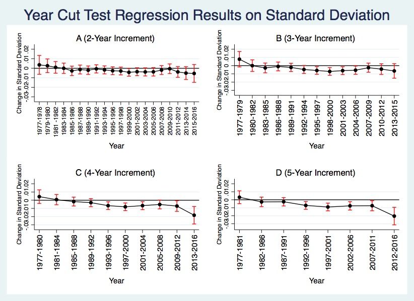
every year. Table 3 presents these groupings. In this regression and subsequent ones, Line

Group serves as the fixed effect, and I cluster standard errors at the Line Group level. Thus,

I am able to identify changes from variation within each line over time rather than the

variation across all lines in order to mitigate omitted variable biases. The specification uses

analytic weights, corresponding to the Line Group’s frequency of occurrence in each time

period.

 While the first set of regressions tests accuracy, the second set tests precision by

capturing the change in the standard deviation of the absolute error over time. The standard

deviation of each Line Group’s prediction error is calculated over 2 to 5-year increments.

Observations are again weighted by the number of games in each Line Group over the

appropriate time interval. The regression equation is

 #,% = ( + * % + ∑23
 #4* # Ι# + e#,% , (2)

where si,t is the standard deviation of the absolute error of Line Group i during year group

t, and Yeart, Ii, ei,t. are the same as in Equation 1.

 The third set of regressions uses a period by period “cut test” to identify periods

after which the standard deviation significantly differs from the prior periods. This test is

performed over 2, 3, 4, and 5-year periods for robustness. The resulting regression equation

is

 #,% = ( + ∑23 23
 #4* # Ι# ∗ Y% + ∑#4* # Ι# + e#,% , (3)

where Yt is a dummy variable that equals 1 if the observation occurs during or after year

group t and 0 otherwise. For instance, let period j represent the 1989 – 1991 seasons when

considering the 3-year increment sample. Pre-1989 games are assigned a value of 0, while

1989 games and afterwards are assigned a value of 1. Standard deviations are calculated

 17

accordingly and regressed on the dummy variable, using Line Group again as the fixed

effect and weighting according to number of games. The remaining variables are defined

as in the previous equations.

Information Assimilation

 As more games are played over the course of a season, market participants have

more information concerning true team ability, and, therefore, performance forecasts

should align more closely with the results of actual performance. The subsequent

regressions give insight into the rate at which the market incorporates such information

into its forecasts of performance by regressing prediction error on the total number of

regular season MLB games that have been played up to that point in time. In these analyses,

I do not use Line Groups; rather, I consider each week’s prediction accuracy in aggregate.

Concern about sample size is the primary motivation behind this decision. Many Line

Groups do not have games in every week of the season, and in the weeks that they are

represented they suffer from small sample sizes - typically fewer than 6 games per week.

Therefore, relying on the assumption that in-season learning occurs across all moneylines

at similar rates, I focus on the week’s predictions in aggregate, using a sample size of 79

games per week on average.

 For every week, I average the implied probability of a favorite win for all games

occurring during that week and compare that to the actual proportion of games won by the

favorite, taking the absolute value of the difference between the two values to calculate

each week’s absolute prediction error. The primary regression equation is

 #,% = ( + * N#,% + ∑92
 %4* % % + e#,% , (4)

 18

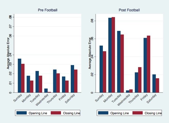
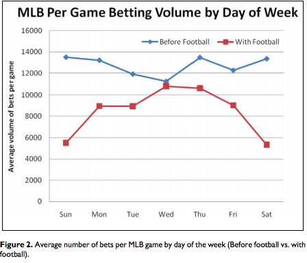
where Ei,t is the absolute error of week i in year t, Ni,t is the total number of games that have

been played before week i of year t, It is an indicator for year t, and ei,t is the error term. I

use year fixed effects in order to control for factors that vary across year, minimizing

potential biases in the estimates that could arise from certain seasons being largely

mispriced. The number of games per week serves as the weight.

 The next two regressions follow Paul and Weinbach (2011), who find that MLB

betting volume decreases substantially after the arrival of the National Football League

(NFL) season, especially on popular NFL game days (Saturday, Sunday, Monday).11

Figure 3 displays the average number of bets per MLB game by day of the week for the

2009 season, both pre- and post-football.12 Betting volume falls in every day of the week

post-football, with the most drastic falls occurring on the weekends. I attempt to exploit

this finding to disentangle the impacts of betting volume and the presence of informed or

“skilled” bettors on line accuracy. It is assumed that a higher volume of bets means that

lines become representative of more people’s beliefs, thereby incorporating more

information. However, if there are a large number of recreational or “uninformed” bettors,

this information could actually be noise. Therefore, studying accuracy post-football can

yield insights into the composition of the betting market, as those still participating are far

likelier to be informed, professional gamblers who are more adept at incorporating

information into their predictions. These bettors remain in the market because they perceive

11
 Paul and Weinbach (2011) show this trend in betting volume only in the 2009 season. I assume that such
trends persist in each season, which is a potential limitation, as it could decrease the meaningfulness of my
findings if the 2009 season was an anomaly.
12
 Pre-football refers to MLB games that occur before the start of NFL season, and post-football refers to
games that occur after the start of the NFL season.

 19

themselves to have an edge and do not change markets due to relatively high switching

costs.

 I perform two additional analyses to capture the impact of the NFL season on

forecasting accuracy and information assimilation in the MLB betting market. The goal of

these analyses is to provide quantitative evidence that can help describe the composition

of bettors and whether it is the informed bettors who drive information incorporation into

the market. The first analysis simply adds a dummy variable to Equation 4 to capture the

difference in accuracy pre- and post-football season. This gives the regression equation

 #,% = ( + * N#,% + 2 #,% + ∑92
 %4* % Ι% + e#,% , (5)

where the additional Fi,t is a dummy variable that equals 1 if week i of year t occurs after

the start of that year’s NFL season and 0 otherwise.13 All other variables are the same as in

Equation 4. I then analyze time trends of these learning rates to see if the rate of information

assimilation has changed over time.

 Next, I analyze prediction at a more granular level: by day of the week. I calculate

the absolute prediction error for every day of the season using the same process as in

Equation 5, but at the daily level instead of weekly. This leads to an average sample size

of 11 games per day. The resulting regression equation is
 *9
 #,% = ( + * N#,% + 2 #,% + ∑92
 %4* % % + ∑#4* # #,% + e#,% , (6)

where Ei,t is now the absolute error of day i in year t, Ni,t is the total number of games that

have been played before day i of year t, It is an indicator for year t (serving as the fixed

effect), and w*F is a series of interaction terms between dummy variables for day of the

13
 For simplicity, if week i of the MLB season begins before the start of the NFL season but still includes the
NFL opening day, I label that week as occurring post-football.

 20

week and a dummy variable for post-football. I repeat this analysis on both the opening

lines and closing lines from the 2013 – 2018 seasons to attempt to determine whether

changes in the market due to football’s arrival are driven by oddsmakers or bettors.

Line Movements

 Lastly, I explore the relationship between line movements and accuracy, focusing

on the impact of overall line movements from opening to closing. After a line opens,

oddsmakers can move it either in response to new information or to imbalances of betting

action, which can be due either to noise generated by uninformed bettors or bettors

responding to their own information. Examples of new information could include line-up

and schedule changes, weather conditions, and injury reports, among many others. I

hypothesize that larger line movements correspond to shifts associated with more

information, thus leading to a higher degree of accuracy. To test this, I calculate the percent

change associated from opening to closing lines, sort games into deciles based on their

percent change, and find the absolute errors associated with both the opening and closing

lines, aggregated by decile.14 To consider the information content of these movements, I

estimate the effect of both their direction and their magnitude on accuracy using the

regression equation

 #,% = ( + * ∆#,% + 2 #,% + > #,% ∗ ∆#,% + 0 #,% + ∑A%4* % % + e#,% , (7)

14
 I choose to focus on percent change instead of other metrics like absolute change in the line because a line
movement of +5 has a far greater impact when the opening line is -130 relative to when the opening line is -
200 (changing the implied probability of a favorite win by -1% and -0.5%, respectively). I therefore assume
that information is likelier to be proportional to percent change in the line rather than absolute shift. Existing
literature only explores the relationship between absolute shifts, market efficiency, and information through
the possible existence of profitable wagering strategies, not through the lens of forecasting accuracy.
Appendix A.4 contains further statistics and information about each decile.

 21

where Ei,t is absolute error associated with the opening line for ith percent change decile in

year t, calculated both pre- and post-football. ∆#,% is the magnitude of the average percent

change of the ith decile in year t, and #,% is a dummy variable equal to 1 if the line moved

towards the favorite or stayed the same and 0 otherwise. ∗ ∆#,% is an interaction term

between magnitude and direction of the line shift. The remaining variables are defined as

above, again using year fixed effects. I repeat the analysis for the closing line as well.

 V. Results

Overall Market Dynamics

 In Table 4, I present results from regressing absolute prediction error on various

time intervals (Equation 1). The coefficient of interest is Year, and its associated coefficient

in the 1-Year column is -0.000823, implying that there is a decline in absolute error over

time, although it is not statistically significant. This estimate suggests that relative to 1977,

out of 100 games valued at a particular Line Group, the favorite would be correctly

predicted 3.45 more times on average in 2018. When aggregating over 2 and 3-year

intervals, the coefficient becomes more negative at -0.00164 and -0.00272, respectively,

with both significant at the 10% level. These estimates are consistent with the favorite

winning 3 to 4 more games on average at a certain Line Group in 2018 compared to 1977.

While the Year coefficients are still negative for the 4 and 5-year intervals, they are no

longer statistically significant, potentially driven in part by the smaller sample size.

 Tables 5 through 9 contain the results from various regressions of standard

deviation of prediction error on time. Firstly, Table 5 displays results from regressing

standard deviation over 2, 3, 4, and 5-year periods (Equation 2). The negative coefficients

signify that the standard deviation of prediction error is decreasing over time, and thus

 22

prediction precision is increasing. As the year increment increases, so does the size of this

effect. For instance, a 4-year increment in time corresponds to a decrease of .00093 in the

standard deviation of prediction error, while a 5-year increment in time corresponds to a

larger decline of .0014, significant at the 1% level. The loss of statistical significance in

the 2-year increment is not surprising, as calculating standard deviation over a sample of

just two observations yields imprecise estimates. Nevertheless, the additional year

increments serve as robustness checks for the downward trend. A possible explanation is

that the market is able to better integrate information over longer periods, increasing

forecasting precision.

 Figure 4 seeks to identify time periods that led to significant changes in the standard

deviation of prediction error over the course of the 42 seasons. The subfigures provide a

visualization of the regression coefficient of interest, Year, and its 95% confidence interval

from the cut tests described in Equation 3. Subplot D of Figure 4 displays the results when

analyzing changes in standard deviation over 5-year periods and shows statistically

significant declines after 1992-1996, 1997-2001, 2002-2006, and 2012-2016 at the 1%

significance level. Comparisons with the results from the 2, 3, and 4-year increment

regressions show that the findings for 1997-2001 and 2002-2006 are robust to the year

increment size and remain significant at least at the 10% level. Table 6 shows that the effect

of decline in standard deviation after 1997-2001 is larger in magnitude (-9.018e-3) than the

decline associated with 2002-2006 (-7.58e-3), signifying a more substantial market shift in

the former period. This finding is again robust to the year increment, as evidenced in Tables

7 through 9.

 23

Overall, these results suggest that there has been a convergence over time between

the market forecasts and actual outcomes. This convergence is primarily due to substantial

improvements in prediction precision rather than prediction accuracy. Marked

improvements in precision occur in the late 1990s and early 2000s, implying that changes

in market dynamics during this time period drive the aggregate trend.

Information Assimilation: Learning Rates Within Season

 The results from regressing weekly absolute error on the running total of games

provide insight into the market’s incorporation of information and are located in Table 10.

The coefficient for running total is -0.0000289 and significant at the 1% level, implying

that the accuracy of lines improves within season. Compared to the first week of a season

(running total = 0), a week towards the end of the season (running total ~ 2200) would have

a prediction error .05358 points smaller, which translates to correctly predicting the

favorite win 4.29 more times on average if the two weeks both have 80 games with the

same distribution of lines. When the dummy variable Post Football is added to the equation,

the coefficient for running total increases slightly in magnitude to -0.0000445 and remains

significant at the 1% level. The coefficient of Post Football is 0.033312, statistically

significant at the 1% level as well, implying that prediction error in the MLB betting market

increases once the NFL season kicks off. This suggests that an 80-game week with games

at the same line just prior the start of the NFL season would correctly predict the favorite

win 2.66 more times on average compared to an 80-game week just after the start of the

NFL season.

 24

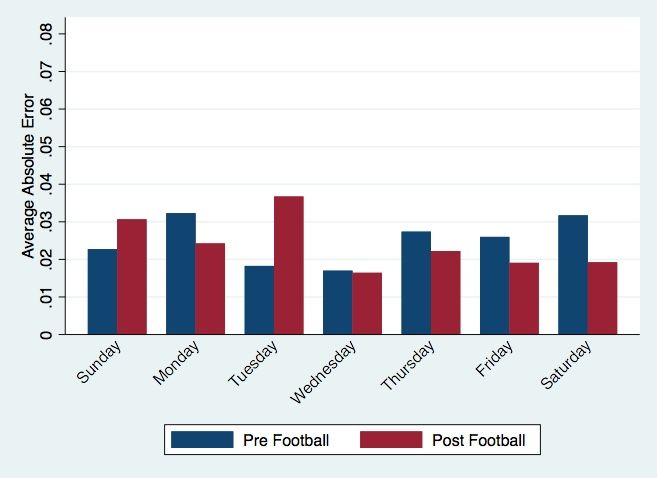
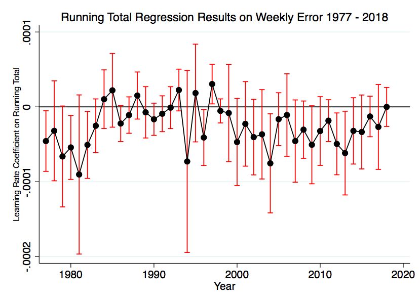
Information Assimilation: Learning Rates Over Time

 Figure 5 displays a plot of the learning rate coefficients, calculated by regressing

weekly error on the running total of games played up to that week for each season from

1977 – 2018, controlling for the start of the football season in each year. When looking at

the sample as a whole, there is no statistically significant downward trend over time, though

in every year from 1998 onwards the coefficient of the running total is negative. The line

of best fit first becomes negative and significant at the 5% level when considering the

period 1982 through 2018.15 Negative values of the learning rate imply that learning does

indeed occur over the course of a season. An overall downward trend in learning rates

would signify that the market incorporates within-season information on performance

faster over time, improving accuracy and leading to a higher degree of efficiency.

However, the evidence is not statistically significant and does not allow us to reject the

hypothesis that learning rates have not changed over time across the period of study.

Information Assimilation: Impact of the NFL Season by Day of the Week

 Graphical analysis of Figures 6 and 7 provides suggestive evidence in support of

the hypothesis that an increase in betting volume alone does not lead to improved accuracy,

with a more important driver being bettor composition.

 Figure 6 displays the average closing line error, aggregated by day of the week,

across the entire 1977 – 2018 sample, while Figure 7 shows the daily opening and closing

line errors from 2013 – 2018. Pre-Football, I consider Saturday, Sunday, Monday, and

Thursday as high-volume, as shown previously in Figure 3. It appears that Pre-Football

high-volume betting days are not the most accurate days in either sample. Rather,

15
 The slope of this best fit line is -8.25 E-7, with a standard error of 3.859 E-7 and R-squared of 0.1156.

 25

Wednesdays, which correspond to the lowest volume days, are. Therefore, it is not simply

the case that more bets lead to better predictions. A possible explanation is that on days

with more bets, there are more recreational gamblers who add noise to the lines and

decrease accuracy. It is also worth noting in these figures that absolute error of lines

increases substantially more after the start of the football season in the years 2013 – 2018

than it does across all seasons. It is possible that sample size is driving this difference, as

relatively few MLB games occur after the start of the football season in each year.

 Further considering the change in volume resulting from the NFL season,

specifically on Saturday and Sunday, appears to show a positive relationship between

informed bettor presence and accuracy improvements. Saturday and Sunday have the

largest decrease in betting volume from Pre-Football to Post-Football, and they, therefore,

likely have the largest concentration of informed bettors Post-Football. Although Saturday

and Sunday do not have the smallest opening and closing line errors Post-Football, they

experience the largest improvements in error reduction from opening to closing lines. This

could suggest that oddsmakers bias their lines Post-Football, especially on Saturdays and

Sundays, in an effort to attract more bettors, and the informed bettors in the market partially

take advantage of this mispricing.

 I test the above hypotheses more rigorously with a regression of error on day of the

week, and Table 11 presents the results. The estimated coefficients do not support the

hypotheses at a statistically significant level. Relative to Saturday in all regressions, the

only days that have worse predictions are Monday and Thursday, significant at the 5%

level. These days have similar betting volumes to Saturdays Pre-Football, and there are no

days with statistically significant improvements in error relative to Saturday. Thus, it does

 26

not appear to be the case that larger betting volumes introduce more noise to lines. In

addition, the coefficient for the change in error on Saturdays Post-Football is positive for

the 2013 – 2018 opening and closing line regressions, and the estimate is not the smallest

for the 1977 – 2018 regression. For instance, the change in error relative to Saturday for

Friday Post-Football is -0.0005422, whereas the change in error for Saturday PostFootball

is -0.000492. However, none of these results are statistically significant. Overall, these tests

are inconclusive at establishing a relationship between betting volume and accuracy and

giving insight into the market composition of bettors.

Line Movements

 Table 12 presents the results from regressing opening and closing absolute error on

line movements. For the opening error results, the point estimate for the magnitude of

percent change is 0.3629, significant at the 1% level. This implies that for games where the

favorite became less favorited, a 1% increase in percent change in the line leads to an

absolute error increase of 0.003629. This estimate is quite small, as it suggests that the

favorite is correctly predicted to win 3.63 more times on average out of 1000 games with

a 4% line change relative to a 5% line change. The effect becomes smaller when

considering closing error, as the point estimate decreases to 0.2526 and remains significant

at the 1% level. This translates to the closing line correctly predicting the favorite win 2.53

more times on average out of 1000 games with a 4% line change relative to a 5% line

change.

 For games where the favorite became more favored, the effect of a 1% magnitude

increase of percent change of the line movement is an increase in opening line error of

0.00163 and a decrease in closing line error of 0.00217. The former result is not statistically

 27

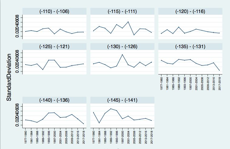
significant, while the latter is significant at the 1% level. Overall, it appears that the

magnitude of the percent change from opening line to closing line has heterogeneous

effects on prediction error, depending on the direction of the shift. If the favorite becomes

more (less) favored, larger shifts are associated with greater (lower) accuracy. It appears

that bettors in the market are able to identify and bet more heavily on favorites undervalued

at the opening line, driving the line to adjust in the appropriate direction in this case.

 Lastly, the coefficient for Post Football is positive for both the opening and closing

error analyses, implying that line error increases after the start of football season. These

results are significant at the 1% level and consistent with the findings in the prior

analyses.16

 VI. Discussion
 Overall, the dominant market dynamic is not improved accuracy of closing lines

over time – there is no statistically significant and robust trend when considering absolute

prediction error. Rather, a decrease in the volatility of the error appears to be driving the

convergence between prediction and actual outcomes. Figures 8 and 9 help demonstrate

this trend among eight of the most frequently occurring moneylines. Substantial

improvements in precision appear to occur after 1997-2001, which provides suggestive

evidence that the increasing quality and quantity of information available for every game

has helped spur this trend. This period corresponds to the takeoff of the internet and the

establishment of free historical databases like Baseball Prospectus and Baseball Reference.

These sites could have served to decrease the cost of data acquisition and processing,

16
 Appendix A.5 provides a sensitivity check to these results, using the line shift as the regressor of interest
instead of percent change. Line shift is the change in implied probability of a favorite win from opening line
to closing line.

 28

thereby mitigating potential inefficiencies that result from data acquisition and processing

barriers (Stigler 1961, Ho and Michaely 1988). For instance, large representative samples

of player performance could be established, providing a more precise view of how players

and teams would fare in certain matchups.

 Additionally, after the 2002 season, the use of sabermetrics proliferated in Major

League Baseball, popularized by the Oakland Athletics’ “Moneyball” strategy. This led 17

to the development of statistics that more accurately predicted player performance and

identified underlying talent levels, enhancing the quality of information in the market

(Passan 2011). In fact, one of the largest and most statistically significant learning rates

corresponds to the 2003 season, implying that the market was able to better incorporate

performance information and thus evaluate team skill more accurately earlier in the season,

making the moneylines better forecasts of actual outcomes. The negative learning

coefficients provide evidence that the market responds to information over the course of

the season – the market is able to assimilate current-season information about team and

individual performances, rather than rely on less representative past performance,

consistent with Ryan et al.’s (2012) findings. Post-2000, there is a general downward trend

in learning rates across seasons, providing suggestive, yet statistically insignificant,

evidence that the information assimilation accelerates over time. Although historical

gambling information is difficult to obtain, a more in-depth comparison of line data, such

as from 1998 to 2004, could perhaps tease out changes in the market as due to information

17
 The Athletics relied heavily on sabermetrics to identify undervalued players, a method known as
“Moneyball”. It helped demonstrate that traditional baseball wisdom is often flawed by overvaluing certain
statistics that in reality weren’t very relevant to player and team performance. With the third lowest payroll
in all of the MLB, the A’s ($40 million) tied the Yankees ($126 million) for most wins and made the playoffs
(Lewis 2003, “MLB Team Payrolls” 2018).

 29

quantity (databases) or information quality (sabermetrics). Another period to study these

information effects could be 2015 onwards, as the 2015 release of StatCast tracks and

makes publicly accessible a tremendous amount of previously unavailable data like exit

velocity, spin rate, and route efficiency. There appears to be clear value in this data, as

MLB front offices invest millions in big data analytics and college teams use similar

technology to try to give their team an edge (Lananna 2018). This value could extend to

the betting market as well, allowing informed bettors who are able to utilize the data to

gain an added edge.

 My findings related to line movements offer interesting contributions to existing

literature in the field. Firstly, the large increase in opening line error after the start of

football season provides suggestive evidence supporting Levitt’s (2004) finding that

oddsmakers intentionally bias their lines in an effort to maximize profit rather than their

traditionally assumed role as market makers. If oddsmakers only consider game attributes

when setting their lines, opening line error is not likely to rise as substantially as it does.

However, a limitation to this aspect of my analysis is sample size, as only about 250 games

occur post-football each season, compared to around 2,150 games pre-football.

Additionally, aggregating error by day of the week could bias my estimates upward. For

instance, a day where two favorites that are valued at 0.6 and 0.65 lost would have a larger

error than a day where two favorites valued at 0.53 and 0.54 lost. But there does not seem

to be a tendency for certain lines to occur on certain days, either pre- or post-football.

Therefore, the bias would be present both pre- and post-football, meaning the increase in

opening line error would still be apparent.

 30