Interstellar Scattering - New diagnostics of pulsars and the ISM Jean-Pierre Macquart
←
→
Page content transcription
If your browser does not render page correctly, please read the page content below
Interstellar Scattering
New diagnostics of pulsars and the ISM

Jean-Pierre Macquart
ICRAR/Curtin University
and
ARC Centre of Excellence for All-sky Astrophysics
The Importance of Interstellar Turbulence
Wisps and sheets of
dust and gas in a giant
star-forming molecular
cloud.
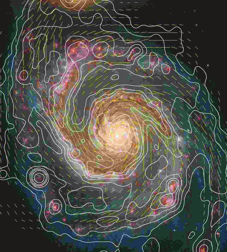
A map of polarization gradients in the Galaxy
reveals turbulent magnetic field structure
(Gaensler et al 2011).
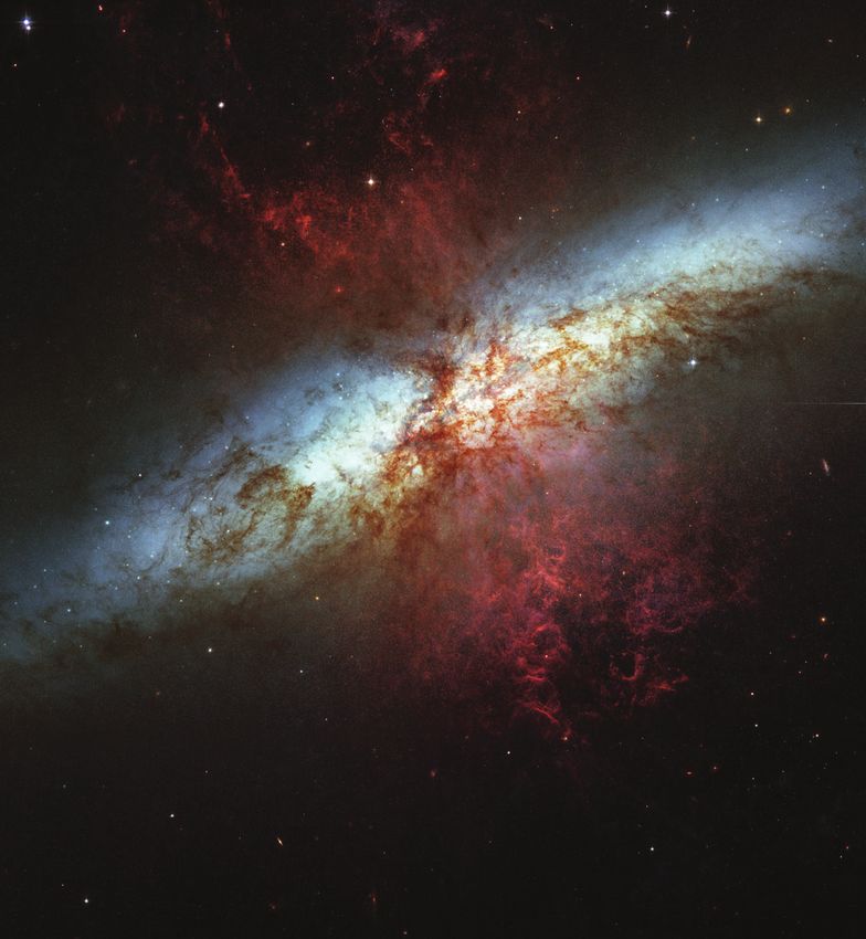
The galaxy M82 spectacularly demonstrates
the relationship between starlight (white), and
turbulent gas (purple).
A map of the diffuse ionized medium across
Turbulence the plane of our Galaxy
Pervades all interstellar space
The energy respository
of massive and dying stars
Drives Galactic magnetic field
The magnetic field of a galaxy like our own.
Regulates star formation (stars and
planets like our Sun and Solar System) The distribution of turbulent neutral hydrogen
This field is created by a dynamo in a small section of our Galaxy.
process that is driven by turbulence. Distorts background radio sources,
causes intensity time variations
The remains of an
Like the twinkling of stars through Earth’s atmosphere, exploded massive star.
the radio quasar J1819+3845 varies when its emission
propagates through interstellar turbulence
(Macquart & de Bruyn 2007).
2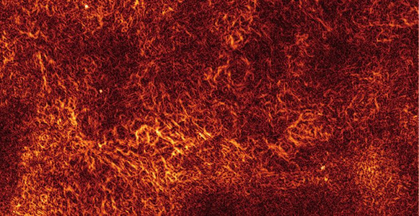
The Standard “Model” for structure
          in the Ionized ISM
The ionized Interstellar Medium of
our Galaxy follows a power law on
scales 106m up to 1014-1018m

The slope of the spectrum is

                                                                   n
                                                               io
surprisingly close to the value

                                                              lat
                                                             til
expected for Kolmogorov turbulence,

                                                         cin
β=11/3.

                                                        rs
                                                       lsa
                                                   pu
                                                   m
                                              fro
                                              ed
                                           riv
    Armstrong, Rickett & Spangler 1995   de
Unresolved Puzzles
        our view of the interstellar turbulence is incomplete

• Extreme Scattering Events
   – Overdense structures?
      • should explode
   – Current sheets?

• Hyperstrong scattering at the Galactic Centre

• The Intermittency of Intra-Day Variability in quasars
• Extremely anisotropic turbulence

                                                          4
0
a4
j2r N D
e 0 \
A B
JjD 2 1
jr N .
impact parameter of R/2, along with the data for 0954!65
To simulate
(14) the nonzero size of the real source, the theoretic
na2 a n e 0
curvestheare smoothed by convolution with Gaussian function
Extreme
We have written a in this second form to emphasize
essential physics. The phase advance through the lens is
The adopted source model corresponds to 50% of the sourc
jr N /n. The Fresnel scale is (jD)1@2. Thus, the properties of
e 0
the lens are determined by the square of the flux ratio of being
the contained within a compact (lensed) componen
Scattering Events
Fresnel scale to the lens size and the phase advance through
the lens. The larger the parameter a, the greater with are this
the component having a brightness temperature of 8 #
observable e†ects due to the lens. Hence a weak 11 lens,
jr N /n > 1, can produce large observable e†ects 10 if the K.
e 0 scale is sufficiently larger than the lens size. Simi-
Fielder et al.
larly,1987
Fresnel
a strong lens, jr N /n > 1, need not produce large
The main qualitative features of these light curves are a
e 0
Goodman etobservable
al. 1987 counted
e†ects if the Fresnel scale is small relative to the for as follows. The phase velocity of the wave is in
lens size. Numerically,
Romani, Blandford & Cordes
a \ 3.6
A j B2A1987 N
0
BA D BA a creaseda
B~2diverging
. (15)
by the presence of free electrons, so the cloud acts a
lens. At low frequencies, the lens is powerf
Walker & Wardle 1998 1 cm 1 cm~3 pc 1 kpc 1 AU
Upon substitution of the above dimensionless enough
variables, that almost all rays are refracted out of the line of sigh
Refractive or Diffractive, Planar, the following expressions are derived for the
properties of a Gaussian lens :
and
the
only a small flux is measured when the lens is aligned wi
refractive
source; this behavior is generic to all blobs of free electron
h (u)/h \ [au exp ([u2) ; (refraction angle) (16)
cylindrical or spherical? r l
u[1 ] a exp ([u2)] [ c \ 0 ; (ray path)
G \ [1 ] (1 [ 2u2)a exp ([u2)]~1 ; (gain factor)
regardless
quently,
(17)
of the details of their density distribution. Cons
(18) this regime of a very strong lens is not particular
k k k
n P `= helpful in distinguishing our model from other possible electro
I(u@, a) \ ; B(b )G (u@, a, b )db . (total intensity)
s k s s density distributions. At higher frequencies, however, the r
k/1 ~=
Refractive models require electron densities (19)
>1000 cm-3 in 0.3-1 AU sized clouds
. CHARACTERISTIC LIGHT CURVE PRODUCED BY A
4 FIG. 2.ÈSchematic diagram of refraction by a Gaussian plasma lens.
See ° 4.1 for a complete description of this Ðgure.
GAUSSIAN LENS
When transverse motion between source, lens, and obser-
ver is assumed, e.g., motion of the observer along the u@ axis,
I(u@, a) translates into a light curve I(u@, a ; t, v), since
Implies extreme thermodynamic properties; u@(t) \ u@(t \ 0) ] vt, where t is time and v is the relative
transverse velocity. We will show that interpretation of
In the limit of geometrical optics, the rays of energy Ñux
travel perpendicular to the constant-phase surfaces. The
direction of travel of the rays is indicated schematically by
>103 overpressured wrt normal ISM. radio light curves in terms of plasma lenses that can be
approximated as Gaussian in proÐle can lead to inferences
the small arrows in the Ðgure. Extending this concept, we
have drawn the path of approximately 100 rays as they
regarding the physical properties of the lens. travel perpendicular to the constant-phase surface after
emergence from the lens. The ray path is shown for a total
4.1. General Description distance D along the lens axis. An observer located close to
We will present numerical results in the following sec- the lens plane but far from the lens axis (e.g., the upper left
Such clouds should be short-lived, making tions. Here we will Ðrst develop a physical understanding
for the basic characteristics of refraction by a Gaussian
and upper right regions of the ray trace) sees an unchanged
source : There is no change in the observed Ñux density (no
them much less common than is observed plasma lens (Fig. 2). Plane waves from an inÐnitely distant
source are incident on the lens screen. The plane waves are
change in the number density of the rays) or in the sourceÏs
position (the direction of arrival of the rays).
indicated by straight dotted lines in the Ðgure, and the lens Somewhat farther from the lens and slightly o†-axis, in
(~0.013 yr-1 source-1) is represented by a plot showing the electron column
density as a function of coordinate u along the lens plane.
the ““ Focusing Regions ÏÏ marked in Figure 2, the rays begin
to converge and their number density increases. An obser-
This representation is purely schematic, as the lens is ver located in this area of the ray trace would see a source of
assumed to have a negligible but uniform width along the enhanced brightness somewhat displaced from its ““ true ÏÏ
line of sight. Upon emergence, the constant-phase surfaces position, as evident from the increased number density and
are distorted into contours that mimic the function N (u), as skewness of the rays, respectively. At the same distance from
e
represented by the inverse GaussianÈshaped dotted lines. the lens, but closer to the lens axis, the rays are spread apart
The lines are inverse GaussianÈshaped because the phase by the lens. An observer in this region would see a source of
velocity is greatest through the center of the lens, where N decreased brightness due to the lower number density of
reaches its maximum value of N . e rays. The source would be o†set from its true position by an
0 5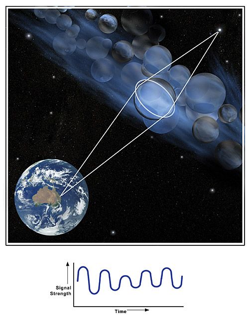
Ionized ISM is highly anisotropic
        and intermittent
The Annual Cycle in J1819+3845
(Dennett-Thorpe & de Bruyn 2003;
Macquart & de Bruyn 2006)     Scattering due to turbulence at ~2pc (!)
                  +(>30)
                                              2
                               of Earth with CN         pc m
                                                > 0.7 ∆L−1   −20/3
Axial ratio     14−8

                                                                  6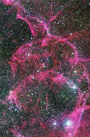
IDV intermittency

                                            Statistics of– Intra-Day
                                                           8–        Variability
                                            from the VLA MASIV survey

Intermittency is the rule:
of the 482 sources surveyed,
only 12% exhibited IDV in all
four epochs

   Lovell et al. 2008
                 Fig. 2.— The variability statistics for the 482 sources surveyed. Sources are divid
                                                                             7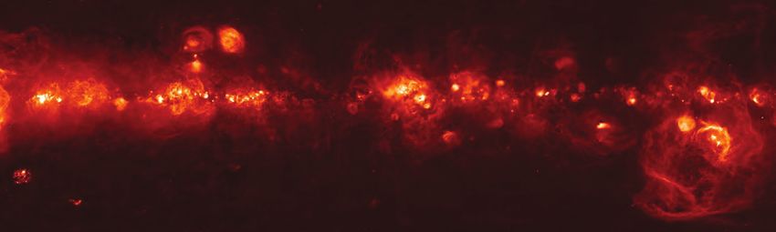
Snapshot speckle imaging
  and ISM holography

   032 "                          3ECONDARY SPECTRUM
  $YNAMIC 3PECTRUM

                      fU tQi2 Qj2

                                    2
                     |FFT|               ft tQi Qj).vscint
                                                    8
Structure in the Secondary Spectrum

delay (conjugate to  Ds ! 2    2
                                 "  φi    φj
  frequency axis) τ=     θi − θj −     +
                     2cβ           2πν   2πν
                       1                        this term usually unimportant
   Doppler shift
(conjugate to time
                   ω=    (θi − θj ) · v⊥
      axis)
                      λβ

                                 •    Interferometry: complex visibility
                                     breaks (ω,τ) (-ω,-τ) symmetry of
                                     intensity sec. spect. The symmetric
                                     part of the phase:
                                                 2πν
                                            ∆φ =     ∆r · (θi + θj )
                                                  c
                                           interferometric baseline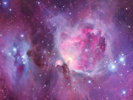
3

                                   Isotropic                          2

                                                                      1
                                                                                       Anisotropic
                 3

                 2
                                                    -3     -2   -1        1    2   3

                 1
                                                                     -1

-3    -2   -1        1    2   3
                                                                     -2

                -1
                                                                     -3
                                                                                            p
                -2                                                                     10
                -3
                                   p
                                  10
                                                                                        8

                                   8

                                                                                        6
                                   6

                                                                                        4
                                   4

                                                                                        2
                                   2

     -4              -2                 2       4        q-4              -2                         2   4
                                                                                                             q
                                              negative delay axis not shown
                                       since secondary spectrum of the intensity is symmetric
                                                 about the delay=0, Doppler=0 axis
                                                                                                10
Brisken Extreme
et al. Scattering
2010 towards PSR B0834+06
The “symmetric”
part of the phaseSpeckle reconstruction
25
20 322.5 MHz
15
10
Relative Declination (mas)
5
0
−5
−10
−15
−20
−25
−30
30 20 10 0 −10 −20
Relative Right Ascension (mas)
12Structure on the primary disk
Does it even follow a 1-D Kolmogorov
– 30 – spectrum?
!0.5
0.5
0
!1
!0.5
!1 !1.5
log10 (B(!))
!1.5
!2
!2
!2.5 !2.5
!3
!3
!3.5
!4 !3.5
30 25 20 15 10 5 0 !5 !10 !15 !20 !25 !8 !9 !10 !11 !12 !13 !14 !15 !16 !17
!|| (mas) ! (mas)
||
Scattered brightness against
Fig. 6.— Left:Scattered θ! along
brightness against the main
θ! obtained for arc. Thethethree
points along over-
main arc via the
plotted curves are for
back-mapped a 1-Din Kolmogorov
astrometry §4.4, averaged from model. The (blue).
all four sub-bands middle curve
The individual
was fitted to the
peaks are observations
as narrow as 0.1 masover
as shownthein range shown
the expanded view ininthegreen. The
right panel. The
other two curves have theoretical
three overplotted the same total
curves flux
(red) are for adensity for Kolmogorov
one-dimensional the pulsar but
model. The
are wider and narrower.
middle curve was fitted to the observations over the range shown in green. The other two
13of a single turbulence model. If rdiff is the length scale spectrum. We
which the RMS phase changes by one radian on this an estimate of
0, each sub-image Off-axis spreads
VLBI Structure
IMAGING radiation into
OF SCATTERING Scattering
anTOWARD
opening ParametersWB: Get
angle
B0834+06
∼ (krdiff )−1 , where k = 2π/λ is the wavenumber. Scat-Table 4 What I want
ng • through
Not a purely “refractive”
an angle 84 mas cloud requires rdiff 2Model = 3.6 Parameters for5Distance and Velocity, Assuming β = 0.353
× 10 m. general in the
322.5 MHz
s is to–beComposed compared of many
with diffractive 3.5 × 10⁷ DmParameter
rdiff 1 = speckles implied by a Value
couple
1171 ± 23 pc
hour
eff
5 min timescale which interfere with those
diffractive on the primaryobserved
scintillations Veff! from 305 ± 3 km s−1
disk and themselves Veff⊥ −145 ± 9 km s−1
primary scattering disk. For a Kolmogorov! Scattering poweraxisspec- −25.2 ± 0.5 deg east of north
• Location does not scale with λ - position is ⊥ Scattering axis −115.2 ±4.3 High
0.5 deg east of north a
m of turbulence this implies a difference in the a scattering
essentially fixed with frequency 3
Ds 415 ± 5 pc
sure by a factor 2.0 × 10 between the two V s!
b
scattering −16
We ± 10 km s−1
now −1 consi
– static structures V s⊥ 0.5 ± 10 km s
s. α sub-images
27 ± 2 deg on
The• 9 present
AU from the ESS primary
detectiondisk, 0.6 AU across
implies a cloudNotes. surface den- theare locations
Note that the first five quantities measured; the
• contributesto
comparable 4%that of thededuced
total scatteredfrompower the rate others ofareExtreme
calculated from these assuming the pulsar distance
of position alo
and velocity as cited in the text.
tering
• Implies Eventsan ESE based on observations
density of 1 per 8x10⁻⁶pc towards
3 extragalac-
a Assumes Dp = 640 pc; the error in Dsintrinsic width
due to the uncertainty
adio(1.3x10
sources. -8pcThe
2 projected),
quasarcomparable
ESE rate to of the Dp is much
0.013 binsource −1larger ∼40%.
yr −1
Including errors from uncertainty in long axis.andTh
pulsar distance
et al. 1987) value
dler quasar-derived is equivalent to one cloud per pro-
proper motion.
metric image
0 −20 0 20 −8 40 2
ed area AESE = 1.9 × 10 (D/1 AU)(vc /50 km s )pc
Doppler (mHz)
−1
, true ratio beca
velocity (>200 km s−1 ) for the scattering screen relativ
re
plottedD is thethe
against typical
Doppler cloudat 322.5
fD for the sub-band diameter
MHz. and
the Sun.vc the cloud low SNR sub-i
with cyan “×”
tromspeed from ESE
marks
across rate
are sampled of 0.013
from source
the inner
-1 -1
main arc inyr (Fiedler
the line of sight. The present observations
a line through
et the1987)
al. 1 ms feature. Black points are from apexes 4.3. Estimating the Image though
Center there a
rclets,aexcept
be cone 1 ms apexes
whose whichradius
are red. a distance D from the observer
In the discussion so far we have assumed itivethat Doppler
the astrom
1/2
τ cD(1 − D/D )] , where τ =is correctly
2 ms iscentered the max- on the emission centroid. However, s
14What about the magnetic field?
Speckle Imaging Relates ne to v and B
• Can track motions of speckles relative to the ISM bulk flow
– Individual motions are ~20% of the mean transverse velocity, requiring high S/
N from bright pulsars to locate the speckles with high precision
• Relation between density and magnetic field is vital to understanding turbulence
– magnetic field fluctuations induce variability in the circular polarization
• speckle-imaging & scintillation-induced circular polarization in B0834+06
probes ~0.001 rad m-2 RM differences on sub-AU scales
RH
LH
plasma wedge
planar incident wavefront
Macquart & Melrose 2000 rotation measure gradient
15Current Sheets
Goldreich & Sridhar (2006), Pen & King (2011)
• ESEs explained in terms of converging underdense regions
– Resolves overpressure problem
– Resolves energetics problem at the Galactic Centre
• Scattering is dominated by the most edge-on current sheet
• BUT such regions are not flux-conserving (it is argued that
ESEs are)
• Projection of the apparently closely-spaced features on
scattering disks
16Lensing from a current sheet
Source moving across the short-axis of the sheet Interst
3 images: two bright and one faint
Positions of all three
images for lensing of a
point-like source
Magnification of all three
images for lensing of a
point-like source
Negative magnification
corresponds to image parity
change, observable in the
pulsar reflex motion
Total magnification if source
is half the size of the lens
17Holography and Phase Retrieval
• We want to find the phases of U(ν,t) based on the dynamic
spectrum: I(ν,t) = U(ν,t) U*(ν,t)
• If we take the Fourier transform of I(ν,t):
˜ ω) = Ũ (τ, ω) # Ũ ∗ (τ, ω)
I(τ,
• ˜ ω) is the autoconvolution of Ũ (τ, ω)
we see that I(τ,
• Decompose the wavefield into a sum of plane waves:
! !
U (ν, t) = uj (ν, t) = ũj e2πi(ντj +ωj t)
j j
delay relative to unscattered wave
Doppler shift, or “fringe rate” in VLBI parlance
• In the Fourier domain:
!
Ũ (τ, ω) = ũj δ(τ − τj )δ(ω − ωj )
jResults
Walker et al. 2008
M. Amplitudes
A. Walker and D.of
R. the scattered
Stinebring wave Comparison
components
iteration (i.e. every time another component wave is From intensity to E-field 1283
e model). Only components whose scale parameters are
n some value (we employed 2 × 10⁻³ ) are included in cisely, the job is to find the phase of U, since the amplitude is known
uares minimization; these criteria mean that 13 scattered directly from I. This emphasizes the importance of a fact mentioned
in the Introduction: this type of problem, i.e. phase-retrieval, has pre-
onents are routinely included. In addition, because the
viously been addressed in various contexts in the optics literature,
wave (τ , ω = 0) is often very strong this component is and future work on dynamic spectrum decomposition should make
ed in the optimization, making 14 wave components in full use of that resource. Our particular application corresponds to
the problem of retrieving a ‘complex-valued object’√ !)
(in our case, U
dual ‘freeze-out’ of component amplitudes, as the from the modulus of its Fourier transform (|U | = I ); this is rec-
le parameter gradually decreases, was incorporated into ognized as a difficult problem (McBride et al. 2004). An acceptable
hm in order that components with similar amplitudes model should yield noise-like residuals (in both dynamic and sec-
multaneously adjusted (optimized) in an efficient way. ondary spectra), and should satisfy the constraint that the number of
free parameters be very much less than the number of independent
of the algorithm has an additional benefit: it helps to
st the possibility of spurious parameter determinations
Data Model
measurements of the dynamic spectrum. Our current algorithm fails
on the first of these criteria. We expect that a globally optimized so-
m local, rather than global minima found by AMOEBA. lution – in which all free parameters are simultaneously adjusted –
finds a local minimum, with correspondingly erroneous would come much closer to achieving noise-like residuals, but
amplitudes, on a given iteration, it may well find its way we have not yet demonstrated this. With such a large number of
ocal minimum to reach the global minimum on the next free parameters, a global optimization would be computationally
cle. Only one of the 14 component amplitudes ceases challenging.
ed on each cycle, so the algorithm has a fair degree of An important limitation of the algorithm we have presented is
that it is restricted to finding scattered waves with τ " 0. Under
o the potential problems caused by local minima in the
many circumstances, this limitation does not cause problems. How-
urface. If, for some reason, the algorithm were to fix a ever, if there are multiple refracted images19present then problems
amplitude at a value that is badly in error, then that errorE1 E1 E1
Pulsar size & Reflex motion 10
• Interference between disks 1 & 2 occurs on a projected
1a baseline of r=1.27x10¹²m. Pulsar emission region less
5
than ~850 km. RA offset mas
20 15 10 5 5
2a
EE*=E1E1*+E1E2*+E2E1*+E2E2* • Closure amplitude: four-element interferometer:
5
1b visibility amplitude on 1a-1b, 1-2 and 2a-2b baselines
measured from the amount of scattered power visible
10
2b in the secondary spectrum associated with each of
Delay s
0.0010
these features.
•
0.0008
The pulsar is substantially resolved if
0.0006
P1−1 P2−2
R= 2 >1 0.03
0.0004 P1−2
0.0002
0.02
Doppler Rate Hz
0.06 0.04 0.02 0.00 0.02 0.04 0.06
illustration of the scattering geometry that gives rise to the observed secondary spectrum. Interference between
• Reflex motion: combine scintillations
elds from the various regions gives rise to distinct features in the secondary spectrum. Bottom: the features in the
that correspond to interference between the wavefields of the two associated scattering regions. Note that no attempt
coherently (using holography) for maximum
oduce the detailed structure of the observed secondary spectrum.
0.01
S/N. Determine phaseTheshift
nterference between the primary and sec-
in Sec Spect as
spur width is related to the shape of the speckle
disks yieldsa
anfunction
offset Θ = 20.7of
masDoppler
from shift and
distribution in the with
ESS. A pulse
narrow spur arises from a lin-
3
Based on the range of observed delays of ear feature and a broad spur from a more circular feature.
phase.
the secondary spectrum, the difference A quantitative measure is obtained using eq. (6) given v 0
0 0.5 1 1.5 2 2.5
t point in the secondary disk to its far- and β2 . The speckle distribution hence has a dispersion of gate separation
e to the image centre is ∆θ = 1.19 mas, 0.81 mas (0.39 AU at the ESS distance) resolved along the
linear size 0.60 AU. direction of v. This is considerably smaller than its 0.60 AU 20Conclusions
• Anomalous scattering in the ISM may be more the norm than the exception
– What causes anomalous scattering in the ISM? What processes in the
dynamics of the Galaxy is it related to?
• Speckle imaging and holography are probe
– pulsars on the nano-arcsecond scale --- pulsar reflex motions
– interstellar turbulence on scales from ~50 AU down to ~109m
• What is the relation between magnetic field, velocity and density fluctuations in
the ISM?
– Density fluctuations observed arise as a by-product of v and B
– A direct discriminant of the various turbulence theories
Current intensity and magnetic field
lines in a simulation of the flow of
an electrically conducting fluid
21Sub-microarcsecond probes of AGN jets
Macquart et al. submitted
PKS 1257-326, ATCA, 2011 Jan 15
0.24
0.22
Flux density (Jy)
0.20
#""
0.18
4540 MHz 5564 MHz 8040 MHz 9064 MHz
4668 MHz 5692 MHz 8168 MHz 9192 MHz !""
4796 MHz 5820 MHz 8296 MHz 9320 MHz
0.16 4924 MHz 5948 MHz 8424 MHz 9448 MHz
5052 MHz 6076 MHz 8552 MHz 9576 MHz *+,- .//0-1 0
5180 MHz 6204 MHz 8680 MHz 9704 MHz &""
5308 MHz 6332 MHz 8808 MHz 9832 MHz
5436 MHz 6460 MHz 8936 MHz 9960 MHz
0.14 %" """ "
16 18 20 22 24 %" """
Time (hr UT) $"""
Jet core-shift scales as ν-0.1 and ν% '()
$"""
#""" ν& '()
diameter as ν-0.6 #"""
Not explainable in terms of the usual !""" !"""
Blandford-Konigl jet model. Requires a
jet traversing a steep pressure gradient
22You can also read