U2020 X-Series USB Peak and Average Power Sensors
←
→
Page content transcription
If your browser does not render page correctly, please read the page content below
DATA SHEE T

U2020 X-Series
USB Peak and
Average Power Sensors
Accelerate Your Production Throughput

                                        Accelerate your production throughput with
                                        Keysight Technologies, Inc. U2020 X-series USB
                                        peak and average power sensors. These sensors
                                        provide the high performance and features
                                        needed to satisfy the requirements of many power
                                        applications in R&D and manufacturing, offering
                                        a fast measurement speed of > 25,000 readings/
                                        second to reduce testing time and cut cost of
                                        test. The U2020 X-series comes with two models:
                                        U2021XA (50 MHz to 18 GHz), and U2022XA
                                        (50 MHz to 40/50 GHz). Get the peak power
                                        measurement capability of a power meter in a
                                        compact, portable form with the Keysight U2020
                                        X-series USB power sensors.

Find us at www.keysight.com                                                        Page 2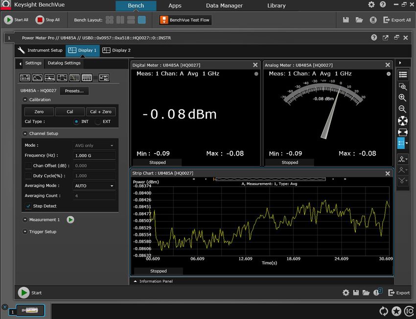
Accurate RMS power                           Built-in trigger in/trigger out
measurements                                 An external trigger enables accurate triggering of small signals close to the signal
The U2020 X-Series have a wide 30 MHz        noise floor. The U2020 X-series USB power sensors come with built-in trigger in/out
video bandwidth and a 80 M-sample/s          connection, allowing you to connect an external trigger signal from a signal source or
continuous sampling rate for fast,           the device-under-test directly to the USB sensor through a standard BNC to SMB cable.
accurate and repeatable RMS power            The sensors also come with recorder/video-output features.
measurements. With its high frequency
coverage of 50 GHz, wide dynamic range       Compact and portable form factor
and extensive measurement capability,
                                             The U2020 X-Series are standalone sensors that operate without the need of a power
the X-Series is optimized for aerospace/
                                             meter or an external power supply. The sensors draw power from a USB port and do not
defense, wireless communication (LTE,
                                             need additional triggering modules to operate, making them portable and lightweight
WCDMA, GSM) and wireless networking
                                             solutions for field applications such as base station testing. Simply plug the sensor to
applications (WLAN).
                                             the USB port of your PC or laptop, and start your power measurements.

A wide peak power dynamic                    The U2020 X-Series is supported by the Keysight BenchVue software and BV0007B
range                                        Power Meter/Sensor Control and Analysis app. Once you plug the USB power sensor
                                             into a PC and run the software you can see measurement results in a wide array of
The U2020 X-series sensors’ dynamic
                                             display formats and log data without any programming.
range of –30 to +20 dBm for peak power
measurements enables more accurate
                                             For more information, www.keysight.com/find/BenchVue
analysis of very small signals, across a
broader range of peak power applications
in the aerospace, defense and wireless       Fast rise and fall time; wide video bandwidth
industries.                                  Accurately measure the output power and timing parameters of pulses when designing
                                             or manufacturing components and subcomponents for radar systems. The U2020
Internal zero and calibration                X-series USB power sensors come with a 30 MHz bandwidth and ≤ 13 ns rise and fall
                                             time, providing a high performance peak and average power solution that covers most
Save time and reduce measurement
                                             high frequency test applications up to 50 GHz.
uncertainty with the internal zero and
calibration function. Each U2020 X-series
sensor comes with technology that            Built-in radar and wireless presets
integrates a DC reference source and         Begin testing faster; the U2020 X-series USB power sensors come with built-in radar
switching circuits into the body of the      and wireless presets for DME, GSM, EDGE, CDMA, WCDMA, WLAN, WiMAX™, and LTE.
sensor so you can zero and calibrate the
sensor while it is connected to a device
under test. This feature removes the need
for connection and disconnection from an
external calibration source, speeding up
testing and reducing connector wear and
tear.

The internal zero and calibration function
is especially important in manufacturing
and automated test environments where
each second and each connection counts.

 Find us at www.keysight.com                                                                                                    Page 3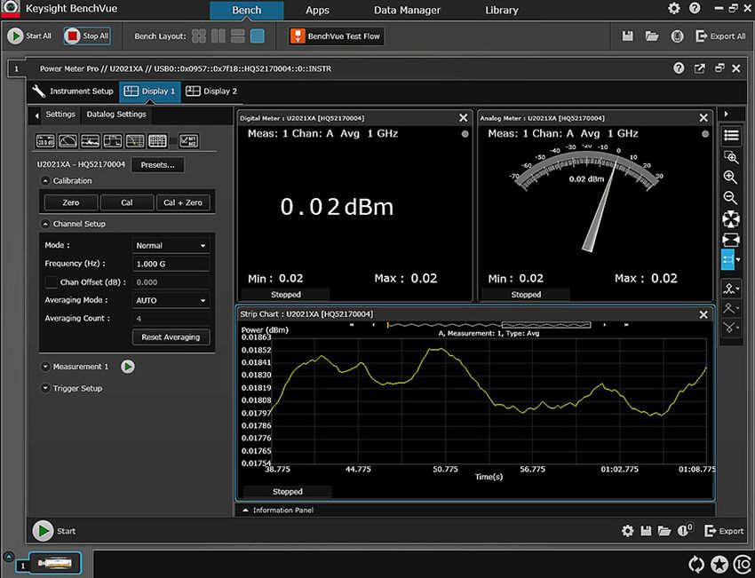
Complementary cumulative                      Additional U2020 X-Series features
distribution function (CCDF)                  List mode
curves
                                              List mode is a mode of operation where a predefined sequence of measurement steps
CCDF characterizes the high power             can be programmed into the power sensor and repeatedly executed as many times as
statistics of a digitally modulated signal,   required. This mode is suitable for power and frequency sweeps which normally require
and is defined by how much time the           changing the parameters via the appropriate SCPI commands before performing a
waveform spends at or above a given           measurement. The hardware handshaking communication between the power sensor
power level. The U2020 X-series supports      and the signal source provides the fastest possible execution time in performing the test
two types of CCDF curves. Normal CCDF         sequences.
displays the power statistics of the whole
waveform under free run, internal or          List mode enables users to setup the number of measurements, the number and
external trigger modes. Gated CCDF can        duration of timeslots, the start and stop frequency for sweeping and the exclusion
be coupled with a measurement gate and        interval. This is especially useful for speeding up measurements for eight time-slotted
only the waveform within the gated region     GSM/EDGE bursts, LTE-TDD or WLAN frames and sub-frames.
is analyzed statistically. Gated CCDF is
only applicable in internal trigger and       For more information, please refer to the programming examples in the U2020 X-Series
external trigger modes.                       Programming Guide.

Designers of components, such as power
                                              Variable aperture size
amplifiers, will compare the CCDF curves
of a signal at the amplifier’s input and      In average only mode and at normal measurement speed, the time interval length used
output. A well designed component             to measure the average power of the signal can be adjusted by setting the aperture size
will produce curves that overlap each         to between 125 µs and 200 ms. This is useful for CW signals and noise-like modulated
other. If the amplifier compresses the        signals such as LTE-FDD and WCDMA by performing measurements over the full frames
signal, then the peak-to-average ratio        or sub-frames.
of the signal will be lower at the output
of the amplifier. The designer will need      Decreasing the aperture size will improve the measurement throughput but reduce the
to improve the range of the amplifier to      signal-to-noise ratio of the measured signal. However, increasing the aperture size will
handle high peak power.                       improve the signal-to-noise ratio of the measured signal but reduce the measurement
                                              throughput.

                                              Table 1. Aperture size
                                               Measurement speed            Default aperture size         Adjustable
                                               NORMal                       50 ms                         Yes
                                               DOUBle                       26 ms                         No
                                               FAST                         2 ms                          No

 Find us at www.keysight.com                                                                                                      Page 4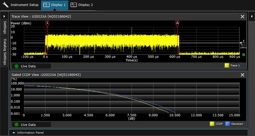
Average only mode external                    High average count reset
trigger                                       When high averaging factors have been set, any rapid adjustments to the amplitude of
The U2020 X-Series also supports              the measured signal will be delayed due to the need to allow the averaging filter to fill
external trigger in average only mode.        before a new measurement can be taken at a stable power level. The U2020 X-Series
The external trigger can be used to           allows you to reset the long filter after the final adjustment to the signal’s amplitude has
synchronize the measurement capture           been made.
with signal burst timing. By adjusting the
aperture size and trigger delay, users        Gamma correction
have greater control on which portion
                                              In an ideal measurement scenario, the reference impedance of the power sensor and
of the waveform is being measured. This
                                              DUT impedance should equal the reference impedance (Zo); however, this is rarely the
function complements the time-gated
                                              case in practice. The mismatch in impedance values results in a portion of the signal
function in normal mode (peak mode) by
                                              voltage being reflected, and this reflection is quantified by the reflection coefficient or
offering a wider power range and faster
                                              gamma.
measurement speed, although it comes
without trace display.
                                              Using gamma correction function, users can simply input the DUT’s gamma into
                                              the sensor via SCPI commands for mismatch correction. This yields more accurate
Auto burst detection                          measurements.
Auto burst detection helps the
measurement setup of the trace or             S-parameter correction
gate positions and sizes, and triggering
                                              Additional errors are often caused by components that are inserted between the DUT
parameters on a large variety of complex
                                              and power sensor, such as in base station testing where a high power attenuator is
modulated signals by synchronizing to
                                              connected between the sensor and base station to reduce the output power to the
the RF bursts. After a successful auto-
                                              measurable power range of the sensor.
scaling, the triggering parameters such
as the trigger level, delay, and hold- off
                                              The S-parameters of these components can be obtained with a vector network analyzer
are automatically adjusted for optimum
                                              in the touchstone format, and inputted into the sensor using SCPI commands. This
operation. The trace settings are also
                                              error can be corrected with the S-parameter correction so that the sensor will measure
adjusted to align the RF burst to the
                                              as though it is connected directly to the DUT, giving users highly accurate power
center of the trace display.
                                              measurements.

20-pulse measurements
The U2020 X-Series can measure up to
20 pulses. The measurement of radar
pulse timing characteristics is greatly
simplified and accelerated by performing
analysis simultaneously on up to 20
pulses within a single capture. Individual
pulse duration, period, duty cycle and
separation, positive or negative transition
duration, and time (relative to the delayed
trigger point) are measured. The U2020
X-Series also supports automatic pulse
tilt (or droop) measurements via SCPI
command.

 Find us at www.keysight.com                                                                                                         Page 5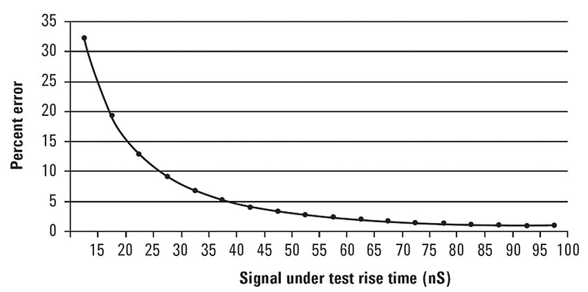
Performance Specifications

Specification definitions                       Characteristic information is representative of the product. In many cases, it may also be
                                                supplemental to a warranted specification. Characteristics specifications are not verified
There are two types of product                  on all units. There are several types of characteristic specifications. They can be divided
specifications:                                 into two groups:
  –– Warranted specifications are
     specifications which are covered           One group of characteristic types describes ‘attributes’ common to all products of a
     by the product warranty and                given model or option. Examples of characteristics that describe ‘attributes’ are the
     apply over a range of 0 to 55 °C           product weight and ‘50-Ω input Type-N connector’. In these examples, product weight
     unless otherwise noted. Warranted          is an ‘approximate’ value and a 50-Ω input is ‘nominal’. These two terms are most widely
     specifications include measurement         used when describing a product’s ‘attributes.’
     uncertainty calculated with a 95%
     confidence.                                The second group describes ‘statistically’ the aggregate performance of the population
  –– Characteristic specifications are          of products. These characteristics d escribe the expected behavior of the population
     specifications that are not warranted.     of products. They do not guarantee the performance of any individual product.
     They describe product performance          No measurement uncertainty value is accounted for in the specification. These
     that is useful in the application of the   specifications are referred to as ‘typical.’
     product.

                                                Conditions
                                                The power sensor will meet its specifications when:
                                                 –– Stored for a minimum of two hours at a stable temperature within the operating
                                                    temperature range, and turned on for at least 30 minutes
                                                 –– The power sensor is within its recommended calibration period, and
                                                 –– Used in accordance to the information provided in the User’s Guide.

 Find us at www.keysight.com                                                                                                         Page 6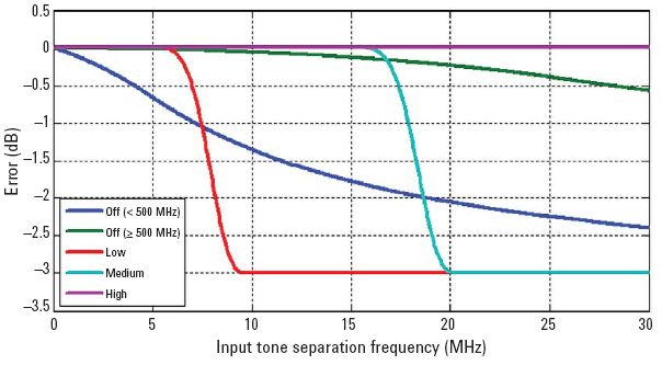
U2020 X-Series USB Power Sensors Specifications

 Key specifications
 Frequency range                                        U2021XA                                            50 MHz to 18 GHz
                                                        U2022XA                                            50 MHz to 40 GHz
                                                                                                           50 MHz to 50 GHz (with Option H50)
 Power range                                            Normal mode                                        –30 dBm to 20 dBm (50 MHz to  40 GHz to 50 GHz)
                                                        Average only mode 1, 2                             –45 dBm to 20 dBm (50 MHz to 40 GHz)
                                                                                                           –45 dBm to 8 dBm (> 40 GHz to 50 GHz)
 Damage level                                           23 dBm (average power)
                                                        30 dBm (< 1 μs duration) (peak power)
 Rise/fall time                                         ≤ 13 ns 3
 Maximum sampling rate                                  80 Msamples/sec, continuous sampling
 Video bandwidth                                        ≥ 30 MHz
 Single-shot bandwidth                                  ≥ 30 MHz
 Minimum pulse width                                    50 ns 4
 Basic accuracy of average power measurement 5          U2021XA                                            ≤ ± 0.2 dB or ± 4.5%
                                                        U2022XA                                            ≤ ± 0.3 dB or ± 6.7%
 Maximum capture length                                 1 s (decimated)
                                                        1.2 ms (at full sampling rate)
 Maximum pulse repetition rate                          10 MHz (based on 8 samples/period)
 Connector type                                         U2021XA                                            N-type (m)
                                                        U2022XA                                            2.4 mm (m)

1. Internal zeroing, trigger output, and video output are disabled in average only mode.
2. It is advisable to perform zeroing when using the average path for the first time after power on, significant temperature changes, or long periods since the
    last zeroing. Ensure that the power sensor is isolated from the RF source when performing external zeroing in average only mode.
3. For frequencies ≥ 500 MHz. Only applicable when the Off video bandwidth is selected. Add 5 ns to rise/fall time specifications for acquisitions smaller than
    137.5 µs.
4. The Minimum Pulse Width is the recommended minimum pulse width viewable, where power measurements are meaningful and accurate, but not
    warranted.
5. This basic accuracy is valid over a range of –15 to +20 dBm, and a frequency range of 0.5 to 10 GHz, DUT Max. SWR < 1.27 for the U2021XA, and a
    frequency range of 0.5 to 40 GHz, DUT Max. SWR < 1.2 for the U2022XA. Averaging set to 32, in Free Run mode. The accuracy under the other conditions
    can be obtained with the measurement uncertainty calculator available on www.keysight.com/find/u2022xa.

 Find us at www.keysight.com                                                                                                                              Page 7
Measured Rise Time Percentage Error Versus Signal-Under-Test Rise Time
Although the rise time specification is
≤ 13 ns, this does not mean that the
U2021XA/22XA can accurately measure
a signal with a known rise time of 13 ns.
The measured rise time is the root sum of
the squares (RSS) of the signal-under-test
(SUT) rise time and the system rise time
(13 ns):
Measured rise time = √((SUT rise time) 2 +
(system rise time) 2) and the % error is:
% Error = ((measured rise time – SUT rise
time)/SUT rise time) × 100
Figure 1. Measured rise time percentage error versus signal under test rise time.
Power Linearity
Power range Linearity at 5 dB step (%)
25 °C 0 to 55 °C
–20 dBm to –10 dBm 1.2 1.8
–10 dBm to 15 dBm 1.2 1.2
15 dBm to 20 dBm 1.4 2.1
Video Bandwidth
The video bandwidth in the U2021XA/ Video bandwidth setting Low: 5 MHz Medium: 15 MHz High: 30 MHz Off
22XA can be set to High, Medium, Low, Rise time/fall time 1 < 500 MHz < 93 ns < 75 ns < 72 ns < 73 ns
and Off. The video bandwidths stated ≥ 500 MHz < 82 ns < 27 ns < 17 ns < 13 ns 3
below are not the 3 dB bandwidths, as Overshoot 2 < 5%
the video bandwidths are corrected for
optimal flatness (except the Off filter). 1. Specified as 10% to 90% for rise time and 90% to 10% for fall time on a 0 dBm pulse.
Refer to Figure 2, “Characteristic peak 2. Specified as the overshoot relative to the settled pulse top power. Applicable to signal with rise time
≥ 15 ns.
flatness,” for information on the flatness 3. Add 5 ns to rise/fall time specifications for acquisitions smaller than 137.5 µs.
response. The Off video bandwidth
setting provides the warranted rise time
and fall time specifications and is the
recommended setting for minimizing
overshoot on pulse signals.
Find us at www.keysight.com Page 8Recorder Output and Characteristic Peak Flatness
Video Output The peak flatness is the flatness of a peak-to-average ratio measurement for various
tone separations for an equal magnitude two- tone RF input. The figure below refers
The recorder output produces a voltage
to the relative error in peak-to-average ratio measurements as the tone separation is
proportional to the selected power
varied. The measurements were performed at –10 dBm.
measurement and is updated at the
measurement rate. Scaling can be
selected with an output range of 0 to 1 V
and impedance of 1 kΩ.
The video output is the direct signal
output detected by the sensor diode, with
no correction applied. The video output
provides a DC voltage proportional to the
measured input power. The DC voltage
can be displayed on an oscilloscope for
time measurement. The video output
impedance is 50 Ω and the level is
approximately 500 mV at 20 dBm CW.
The trigger out and recorder/video out
share the same port, and the level is
approximately 250 mV at 20 dBm.
Figure 2. U2021XA/22XA error in peak-to-average measurements for a two-tone input (High,
Medium, Low and Off Filters).
Noise and drift
Mode Zeroing Zero set Zero drift 1 Noise per sample Measurement noise
< 500 MHz ≥ 500 MHz < 500 MHz ≥ 500 MHz
Normal No RF on input ± 200 nW ± 100 nW ± 3 μW ± 2.5 μW ± 100 nW 2 (Free run)
RF present ± 200 nW ± 200 nW
Average only No RF on input ± 10 nW ± 6 nW ± 3 μW ± 2.5 μW ± 4 nW 3
Measurement average setting 1 2 4 8 16 32 64 128 256 512 1024
Normal mode Free run noise 1.00 0.9 0.8 0.7 0.6 0.5 0.45 0.4 0.3 0.25 0.2
multiplier
Average only NORMal speed 4.25 2.84 2.15 1.52 1.00 0.78 0.71 0.52 0.5 0.47 0.42
noise multiplier
DOUBle speed 5.88 4.00 2.93 1.89 1.56 1.00 0.73 0.55 0.52 0.48 0.44
noise multiplier
Video bandwidth setting Low: 5 MHz Medium: 15 MHz High: 30 MHz Off
Noise per sample < 500 MHz 0.6 1.3 2.7 1.00
multiplier ≥ 500 MHz 0.55 0.65 0.8 1.00
For average only mode with aperture size of ≥ 12 ms and averaging set to 1, the measurement noise is calculated as follows:
–– Measurement noise = 120/√(aperture size in ms) nW.
–– For average only mode with aperture size of < 12 ms and averaging set to 1, the measurement noise is equal to 50 nW.
–– For example, if the aperture size is 50 ms and averaging set to 1, Measurement noise = 120/√(50) nW = 17 n.
1. Within 1 hour after zeroing, at a constant temperature, after a 24-hour warm-up of the U2020 X-Series. This component can be disregarded with the
auto-zeroing mode set to ON.
2. Measured over a 1-minute interval, at NORMal speed, at a constant temperature, two standard deviations, with averaging set to 1.
3. Tested with averaging set to 16 at NORMal speed and 32 at DOUBLE speed.
Find us at www.keysight.com Page 9Effect of Video Bandwidth Maximum SWR
Setting Frequency band U2021XA U2022XA
The noise per sample is reduced by 50 MHz to 10 GHz 1.2 1.2
applying the video bandwidth filter setting > 10 GHz to 18 GHz 1.26 1.26
(High, Medium, or Low). If averaging is > 18 GHz to 26.5 GHz 1.3
implemented, this will dominate any effect > 26.5 GHz to 40 GHz 1.5
of changing the video bandwidth. > 40 GHz to 50 GHz 1.7
Effect of Time-Gating on
Measurement Noise
The measurement noise for a gated average
measurement is calculated from the noise
per sample specification. The noise for any
particular gate is equal to Nsample/√(gate
length/12.5 ns). The improvement in
noise limits at the measurement noise
specification of 100 nW.
Calibration Uncertainty
Definition: Uncertainty resulting from Frequency band U2021XA U2022XA
non-linearity in the U2021XA/22XA 50 MHz to 500 MHz 4.2% 4.3%
detection and correction process. This > 500 MHz to 1 GHz 4.0% 4.2%
can be considered as a combination of > 1 GHz to 10 GHz 4.0% 4.5%
traditional linearity, calibration factor > 10 GHz to 18 GHz 4.5% 4.5%
and temperature specifications and the > 18 GHz to 26.5 GHz 5.3%
uncertainty associated with the internal > 26.5 GHz to 40 GHz 5.8%
calibration process.
> 40 GHz to 47 GHz (up to +8 dBm only) 7%
> 47 GHz to 50 GHz (up to +8 dBm only) 8%
Note. For power range +8 dBm to +20 dBm within the frequency range of > 40 GHz to 50 GHz, the typical power
measurement error is up to 10% at room temperature (23 °C ± 3 °C).
Find us at www.keysight.com Page 10Timebase and Trigger Specifications
Timebase
Range 2 ns to 100 ms/div
Accuracy ± 25 ppm
Jitter ≤ 1 ns
Trigger
Internal trigger
Range –20 to 20 dBm
Resolution 0.1 dB
Level accuracy ± 0.5 dB
Latency 1 300 ns ± 12.5 ns
Jitter ≤ 5 ns RMS
External TTL trigger input
High > 2.4 V
Low < 0.7 V
Latency 2 212.5 ns ± 12.5 ns
Minimum trigger pulse width 15 ns
Minimum trigger repetition period 50 ns
Maximum trigger voltage input 5 V EMF from 50 Ω DC (current < 100 mA), or
5 V EMF from 50 Ω (pulse width < 1 s, current < 100 mA)
Impedance 50 Ω, 100 kΩ (default)
Jitter ≤ 0.5 ns RMS
External TTL trigger output Low to high transition on trigger event
High > 2.4 V
Low < 0.7 V
Latency 3 50 ns ± 12.5 ns
Impedance 50 Ω
Jitter ≤ 5 ns RMS
Trigger delay
Range ± 1.0 s, maximum
Resolution 1% of delay setting, 12.5 ns minimum
Trigger holdoff
Range 1 μs to 400 ms
Resolution 1% of selected value (to a minimum of 12.5 ns)
Trigger level threshold hysteresis
Range ± 3 dB
Resolution 0.05 dB
1. Internal trigger latency is defined as the delay between the applied RF crossing the trigger level and the U2021XA/22XA switching into the triggered state.
2. External trigger latency is defined as the delay between the applied trigger crossing the trigger level and the U2021XA/22XA switching into the triggered
state.
3. External trigger output latency is defined as the delay between the U2021XA/22XA entering the triggered state and the output signal switching.
Find us at www.keysight.com Page 11General Specifications
Inputs/Outputs
Current requirement 450 mA max (approximately)
Recorder output Analog 0 to 1 V, 1 kΩ output impedance, SMB connector
Video output 0 to 1 V, 50 Ω output impedance, SMB connector
Trigger input Input has TTL compatible logic levels and uses a SMB connector
Trigger output Output provides TTL compatible logic levels and uses a SMB connector
Remote programming
Interface USB 2.0 interface USB-TMC compliance
Command language SCPI standard interface commands, IVI-COM, IVI-C driver and LabVIEW drivers
Maximum measurement speed
Free run trigger measurement 25,000 readings per second 1
External trigger time-gated measurement 20,000 readings per second 2
1. Tested under normal mode and fast mode, with buffer mode trigger count of 100, output in binary format, unit in watt, auto-zeroing, auto-calibration, and
step detect disabled.
2. Tested under normal mode and fast mode, with buffer mode trigger count of 100, pulsed signal with PRF of 20 kHz, and pulse width at 15 µs.
General Characteristics
Environmental compliance
Temperature Operating condition: –0 to 55 °C
Storage condition:–40 to 70 °C
Humidity Operating condition: Maximum: 95% at 40 °C (non-condensing)
Storage condition: Up to 90% at 65°C (non-condensing)
Altitude Operating condition: Up to 3000 m (9840 ft)
Storage condition: Up to 15420 m (50000 ft)
Regulatory compliance
The U2021XA/22XA USB peak power sensor IEC 61010-1:2001/EN 61010-1:2001 (2nd edition)
complies with the following safety and EMC IEC 61326:2002/EN 61326:1997 +A1:1998 +A2:2001 +A3:2003
requirements: Canada: ICES-001:2004
Australia/New Zealand: AS/NZS CISPR11:2004
South Korea EMC (KC Mark) certification: RRA 2011-17
Dimensions (Length × Width × Height) 140 mm × 45 mm × 35 mm
Weight Net weight: ≤ 0.25 kg
Shipping weight: 1.4 kg
Connectivity
USB 2.0, with the following cable lengths: Option 301: 1.5 m
(Selectable during sensor purchase) Option 302: 3 m
Option 303: 5 m
Recommended calibration interval 1 year
Mechanical Characteristic
Mechanical characteristics such as center conductor protrusion and pin depth are not performance specifications. They are, however,
important supplemental characteristics related to electrical performance. At no time should the pin depth of the connector be
protruding.
Find us at www.keysight.com Page 12Using the U2020 X-Series with the BenchVue Software
The U2020 X-Series is supported by
Keysight BenchVue software’s BV0007B
Power Meter/Sensor Control and Analysis
App. Keysight BenchVue software for
the PC accelerates testing by providing
intuitive, multiple instrument measurement
visibility and data capture with no
programming necessary. You can derive
answers faster than ever by easily viewing,
capturing and exporting measurement
data and screen shots. Keysight BenchVue
software license (BV0007B) is now
included with your instrument.
For more information,
www.keysight.com/find/BenchVue
Figure 3. Digital meter, analog meter and datalog view.
BenchVue software’s power meter/sensor control and analysis app
Supported functionality
Measurement displays Digital meter
Analog meter
Data log view
Trace view (up to 4 channels or traces on one graph)
Complementary cumulative distribution function (CCDF) view
Multilist with ratio/delta function
Compact mode display
Graph functions Single marker (up to 5 markers per graph)
Dual marker (up to 2 sets of markers per graph)
Graph autoscaling
Graph zooming
Gate measurement analysis (up to 4-pair of gates)
Pulse characterization 17-point automatic pulse parameters characterization
functions
Instrument settings Save and recall instrument state including graph settings
Instrument preset settings (DME, GSM, WCDMA, WLAN, LTE, etc.)
FDO tables
Gamma and S-parameters tables
Full instrumentation control include frequency/average/trigger
settings, zero and calibration, etc.
Limit and alert function Sensors Limit and alert notification
Alert summary
Export data or screen shots Data logging (HDF5/MATLAB/Microsoft Excel/Microsoft Word/CSV)
Save screen capture (PNG/JPEG/BMP)
Find us at www.keysight.com Page 13System and Installation Requirements
PC operating system
Windows 10, 8 and 7 Windows 10 32-bit and 64-bit (Professional, Enterprise, Education, Home versions)
Windows 8 32-bit and 64-bit (Core, Professional, Enterprise)
Windows 7 SP1 and later 32-bit and 64-bit (Professional, Enterprise, Ultimate)
Computer hardware Professor: 1 GHz or faster (2 GHz or greater recommended)
RAM: 1 GB (32-bit) or 2 GB (64-bit) (3 GB or greater recommended)
Windows XP SP3 32-bit (Professional) Processor: 600 MHz or faster (1 GHz or greater recommended)
RAM: 1 GB (2 GB or greater recommended)
Interfaces USB, GPIB, LAN, RS-232
Display resolution 1024 x 768 minimum for single instrument view (higher resolutions are recommended for multiple instrument
view)
Additional requirements
Software: BenchVue requires a VISA (Keysight or National Instruments) when used to connect to physical instruments. Keysight IO
Libraries, which contains the necessary VISA, will be installed automatically when BenchVue is installed. IO Libraries information is
available at: www.keysight.com/find/iosuite
Find us at www.keysight.com Page 14Ordering Information
Model Description
U2021XA X-Series USB peak and average power sensor, 50 MHz to 18 GHz
U2022XA X-Series USB peak and average power sensor, 50 MHz to 40 GHz
U2022XA-H50 X-Series USB peak and average power sensor, 50 MHz to 50 GHz
Standard shipped Items
–– Power sensor cable 5 ft (1.5 m), default cable length
–– BNC male to SMB female trigger cable, 50 Ω, 1.5 m (Quantity: 2)
–– Certificate of calibration
Options Description
Accessories
U2000A-201 Transit case
U2000A-202 Soft carrying case
U2000A-203 Holster
U2000A-204 Soft carrying pouch
Cables (selectable during sensor purchase)
U2000A-301 Power sensor cable, 5 ft (1.5 m)
U2000A-302 Power sensor cable, 10 ft (3 m)
U2000A-303 Power sensor cable, 16.4 ft (5 m)
Cables (ordered standalone)
U2031A Power sensor cable, 5 ft (1.5 m)
U2031B Power sensor cable, 10 ft (3 m)
U2031C Power sensor cable, 16.4 ft (5 m)
U2032A BNC male to SMB female trigger cable, 50 Ω , 1.5 m
Documentation
Option OB1 English language operating and service guide
Option OBF English language programming guide
Option OBN English language service guide
Option ABJ Japanese language operating and service guide
U2021XA-CD1 Documentation optical disk
(consists of documentation CD-ROM and Keysight instruments control DVD)
Software
BV0007B BenchVue Power Meter/Sensor Control and Analysis app license
Calibration
UK6 Commercial calibration with test data
A6J 1 ANSI Z540 compliant calibration and test data
1A7 1 ISO 17025 compliant calibration and test data
1. Not available for Option H50.
Find us at www.keysight.com Page 15Worked Example
Uncertainty calculations for a power measurement (settled, average power)
(Specification values from this document are in bold italic, values calculated on this page are underlined.)
Process
1. Power level............................................................................................................................................................... 1 mW
2. Frequency................................................................................................................................................................. 1 GHz
3. Calculate sensor uncertainty:
In Free Run, auto zero mode average = 16
Calculate noise contribution
–– If in Free Run mode, Noise = Measurement noise x free run multiplier = 100 nW x 0.6 = 60 nW
–– If in Trigger mode, Noise = Noise-per-sample x noise per sample multiplier
Convert noise contribution to a relative term 1 = Noise/Power = 60 nW/100 µW.............................................. 0.06%
Convert zero drift to relative term = Drift/Power = 100 nW/1 mW..................................................................... 0.01%
RSS of above terms =.............................................................................................................................................. 0.061%
4. Zero uncertainty
(Mode and frequency dependent) = Zero set/Power = 200 nW/1 mW..................................................... 0.02%
5. Sensor calibration uncertainty
(Sensor, frequency, power and temperature dependent) = ......................................................................... 4.0%
6. System contribution, coverage factor of 2 ≥ sysrss =............................................................................................ 4.0%
(RSS three terms from steps 3, 4 and 5)
7. Standard uncertainty of mismatch
Max SWR (frequency dependent) =........................................................................................................................ 1.20
Convert to reflection coefficient, | ρSensor | = (SWR–1)/(SWR+1) =........................................................................ 0.091
Max DUT SWR (frequency dependent) =................................................................................................................ 1.26
Convert to reflection coefficient, | ρDUT | = (SWR–1)/(SWR+1) =........................................................................... 0.115
8. Combined measurement uncertainty @ k=1
( Max (ρDUT ) • Max (ρSensor )
) ( sysrss
)
2 2
UC = ———————————————————— +————— ...............................................................................................
√2 2 2.13%
Expanded uncertainty, k = 2, = UC • 2 =................................................................................................................. 4.27%
1. The noise to power ratio is capped for powers > 100 μW, in these cases use: Noise/100 μW.
Find us at www.keysight.com Page 16Graphical Example
A. System contribution to measurement uncertainty versus power level (equates to step 6 result/2)
Note. The above graph is valid for conditions of free-run operation,
with a signal within the video bandwidth setting on the system.
Humidity < 70 %.
B. Standard uncertainty of mismatch
Standard uncertainty of mismatch - 1 sigma (%) SWR ρ SWR ρ
0.5 1.0 0.00 1.8 0.29
1.05 0.02 1.90 0.31
0.45
1.10 0.05 2.00 0.33
0.4 1.15 0.07 2.10 0.35
1.20 0.09 2.20 0.38
0.35
1.25 0.11 2.30 0.39
0.3 1.30 0.13 2.40 0.41
ρSensor
1.35 0.15 2.50 0.43
0.25 1.40 0.17 2.60 0.44
0.2
1.45 0.18 2.70 0.46
1.5 0.20 2.80 0.47
0.15 1.6 0.23 2.90 0.49
1.7 0.26 3.00 0.50
0.1
0.05
0
0 0.1 0.2 0.3 0.4 0.5
ρDUT
Note. The above graph shows the Standard Uncertainty of Mismatch = ρDUT. ρSensor /√ 2, rather than the Mismatch Uncertainty Limits.
This term assumes that both the Source and Load have uniform magnitude and uniform phase probability distributions.
C. Combine A and B
UC = √ (Value from Graph A) 2 + (Value from Graph B) 2
Expanded uncertainty, k = 2, = UC • 2 = ..................................................................................................................... ± %
Find us at www.keysight.com Page 17Appendix A
Uncertainty calculations for a power measurement (settled, average power)
(Specification values from this document are in bold italic, values calculated on this page are underlined.)
Process
1. Power level............................................................................................................................................................... W
2. Frequency.................................................................................................................................................................
3. Calculate sensor uncertainty:
Calculate noise contribution
– If in Free Run mode, Noise = Measurement noise x free run multiplier
– If in Trigger mode, Noise = Noise-per-sample x noise per sample multiplier
Convert noise contribution to a relative term 1 = Noise/Power =........................................................................ %
Convert zero drift to relative term = Drift/Power =............................................................................................... %
RSS of above terms =.............................................................................................................................................. %
4. Zero uncertainty
(Mode and frequency dependent) = Zero set/Power =...................................................................... %
5. Sensor calibration uncertainty................................................................................................................................
(Sensor, frequency, power and temperature dependent) =.............................................................. %
6. System contribution, coverage factor of 2 ≥ sysrss =............................................................................................. %
(RSS three terms from steps 3, 4 and 5)
7. Standard uncertainty of mismatch
Max SWR (frequency dependent) =.......................................................................................................................
Convert to reflection coefficient, | ρ Sensor | = (SWR–1)/(SWR+1) =.......................................................................
Max DUT SWR (frequency dependent) =...............................................................................................................
Convert to reflection coefficient, | ρDUT | = (SWR–1)/(SWR+1) =..........................................................................
8. Combined measurement uncertainty @ k = 1
( Max(ρDUT) • Max(ρSensor)
) ( sysrss
)
2 2
UC = + ————— %
——————————————————— ...............................................................................................
√2 2
Expanded uncertainty, k = 2, = UC • 2 =................................................................................................................. %
1. The noise to power ratio for average only mode is capped at 0.01% for MU calculation purposes.
Learn more at: www.keysight.com
For more information on Keysight Technologies’ products, applications or services,
please contact your local Keysight office. The complete list is available at:
www.keysight.com/find/contactus
Find us at www.keysight.com Page 18
This information is subject to change without notice. © Keysight Technologies, 2010 - 2020, Published in USA , August 10, 2020, 5991-0310ENYou can also read