INVERTIBLE MANIFOLD LEARNING FOR DIMENSION REDUCTION
←
→
Page content transcription
If your browser does not render page correctly, please read the page content below
Under review as a conference paper at ICLR 2021

I NVERTIBLE M ANIFOLD L EARNING                                        FOR       D IMENSION
R EDUCTION
 Anonymous authors
 Paper under double-blind review

                                            A BSTRACT

         It is widely believed that a dimension reduction (DR) process drops information
         inevitably in most practical scenarios. Thus, most methods try to preserve some
         essential information of data after DR, as well as manifold based DR methods.
         However, they usually fail to yield satisfying results, especially in high-dimensional
         cases. In the context of manifold learning, we think that a good low-dimensional
         representation should preserve the topological and geometric properties of data
         manifolds, which involve exactly the entire information of the data manifolds. In
         this paper, we define the problem of information-lossless NLDR with the mani-
         fold assumption and propose a novel two-stage NLDR method, called invertible
         manifold learning (inv-ML), to tackle this problem. A local isometry constraint
         of preserving local geometry is applied under this assumption in inv-ML. Firstly,
         a homeomorphic sparse coordinate transformation is learned to find the low-
         dimensional representation without losing topological information. Secondly, a
         linear compression is performed on the learned sparse coding, with the trade-off
         between the target dimension and the incurred information loss. Experiments are
         conducted on seven datasets with a neural network implementation of inv-ML,
         called i-ML-Enc, which demonstrate that the proposed inv-ML not only achieves
         invertible NLDR in comparison with typical existing methods but also reveals the
         characteristics of the learned manifolds through linear interpolation in latent space.
         Moreover, we find that the reliability of tangent space approximated by the local
         neighborhood on real-world datasets is key to the success of manifold based DR
         algorithms. The code will be made available soon.

1   I NTRODUCTION
In real-world scenarios, it is widely believed that the loss of data information is inevitable after
dimension reduction (DR), though the goal of DR is to preserve as much information as possible in
the low-dimensional space. In the case of linear DR, compressed sensing (Donoho, 2006) breaks this
common sense with practical sparse conditions of the given data. In the case of nonlinear dimension
reduction (NLDR), however, it has not been clearly discussed, e.g. what is the structure within data
and how to maintain these structures after NLDR? From the perspective of manifold learning, the
manifold assumption is widely adopted, but classical manifold based DR methods usually fail to yield
good results in the many practical case. Therefore, what is the gap between theoretical and real-world
applications of manifold based DR? Here, we give the first detailed discussion of these two problems
in the context of manifold learning. We think that a good low-dimensional representation should
preserve the topology and geometry of input data, which require the NLDR transformation to be
homeomorphic. Thus, we propose an invertible NLDR process, called inv-ML, combining sparse
coordinate transformation and local isometry constraint which preserve the property of topology and
geometry, to explain the information-lossless NLDR in manifold learning theoretically. We instantiate
inv-ML as a neural network called i-ML-Enc via a cascade of equidimensional layers and a linear
transform layer. Sufficient experiments are conduct to validate invertible NLDR abilities of i-ML-Enc
and analyze learned representations to reveal inherent difficulties of classical manifold learning.

Topology preserving dimension reduction. To start, we first make out the theoretical definition
of information-lossless DR on a manifold. The topological property is what is invariant under a
homeomorphism, and thus what we want to achieve is to construct a homeomorphism for dimension

                                                   1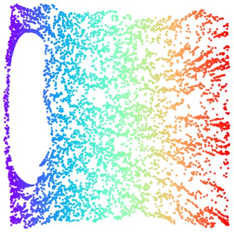
Under review as a conference paper at ICLR 2021

reduction, removing the redundant dimensions while preserving invariant topology. To be more
specific, f : Md0 → Rm is a smooth mapping of a differential manifold into another, and if f is a
homeomorphism of Md0 into Md1 = f (Md0 ) ⊂ Rm , we call f is an embedding of Md0 into Rm .
Assume that the data set X = {xj |1 ≤ j ≤ n} sampled from the compact manifold Md1 ⊂ Rm
which we call the data manifold and is homeomorphic to Md0 . For the sample points we get are
represented in the coordinate after inclusion mapping i1 , we can only regard them as points from
Euclidean space Rm without any prior knowledge, and learn to approximate the data manifold in the
latent space Z. According to the Whitney Embedding Theorem (Seshadri & Verma, 2016), Md0 is can
be embedded smoothly into R2d by a homeomorphism g. Rather than to find the f −1 : Md1 → Md0 ,
our goal is to seek a smooth map h : Md1 → Rs ⊂ R2d , where h = g ◦ f −1 is a homeomorphism
of Md1 into Md2 = h(Md1 ) and d ≤ s ≤ 2d  m, and thus the dim(h(X )) = s, which achieves
the DR while preserving the topology. Owing to the homeomorphism h we seek as a DR mapping,
the data manifold Md1 is reconstructible via Md1 = h−1 ◦ h(Md1 ), by which we mean h a topology
preserving DR as well as information-lossless DR.

Figure 1: Illustration of the process of NLDR. The dash line links Md1 and x means x is sampled
from Md1 , and it is represented in the Euclidean space Rm after an inclusion mapping ii . We aim
to approximate Md1 from the observed sample x. For the topology preserving dimension reduction
methods, it aims to find a homeomorphism g ◦ f −1 to map x into z which is embedded in Rs .

Geometry preserving dimension reduction. While the topology of the data manifold Md1 can
be preserved by the homeomorphism h discussed above, it may distort the geometry. To preserve
the local geometry of the data manifold, the map should be isometric on the tangent space Tp Md1
for every p ∈ Md1 , indicating that dMd1 (u, v) = dMd2 (h(u), h(v)), ∀u, v ∈ Tp Md1 . By Nash’s
Embedding Theorem (Nash, 1956), any smooth manifold of class C k with k ≥ 3 and dimension d
can be embedded isometrically in the Euclidean space Rs with s polynomial in d.
Noise perturbation. In the real-world scenarios, sample points are not lied on the ideal manifold
strictly due to the limitation of sampling, e.g. non-uniform sampling noises. When the DR method is
very robust to the noise, it is reasonable to ignore the effects of the noise and learn the representation
Z from the given data. Therefore, the intrinsic dimension of X is approximate to d, resulting in the
lowest isometric embedding dimension is larger than s.

2    R ELATED W ORK

Manifold learning. Most classical linear or nonlinear DR methods aim to preserve the geometric
properties of manifolds. The Isomap (Tenenbaum et al., 2000) based methods aim to preserve the
global metric between every pair of sample points. For example, McQueen et al. (2016) can be
regarded as such methods based on the push-forward Riemannian metric. For the other aspect, LLE
(Roweis & Saul, 2000) based methods try to preserve local geometry after DR, whose derivatives like
LTSA (Zhang & Zha, 2004), MLLE (Zhang & Wang, 2007), etc. have been widely used but usually
fail in the high-dimensional case. Recently, based on local properties of manifolds, MLDL (Li et al.,
2020) was proposed as a robust NLDR method implemented by a neural network, preserving the local
geometry but abandoning the retention of topology. In contrast, our method takes the preservation of
both geometry and topology into consideration, trying to maintain these properties of manifolds even
in cases of excessive dimension reduction when the target dimension s0 is smaller than s.
Invertible model. From AutoEncoder (AE) (Hinton & Salakhutdinov, 2006), the fundamental
neural network based model, having achieved DR and cut information loss by minimizing the
reconstruction loss, some AE based generative models like VAE (Kingma & Welling, 2014) and
manifold-based NLDR models like TopoAE (Moor et al., 2020) has emerged. These methods
cannot avoid information loss after NLDR, and thus, some invertible models consist of a series of

                                                    2
Under review as a conference paper at ICLR 2021

equidimensional layers have been proposed, some of which aim to generate samples by density
estimation through layers (Dinh et al., 2015) (Dinh et al., 2017) (Behrmann et al., 2019), and the
other of which are established for other targets, e.g. validating the mutual information bottleneck
(Jacobsen et al., 2018). Different from methods mentioned above, our proposed i-ML-Enc is a neural
network based encoder, with NLDR as well as maintaining structures of raw data points based on
manifold assumption via a series of equidimensional layers.
Compressed sensing. The JohnsonLindenstrauss Theorem (Johnson & Lindenstrauss, 1984) pro-
vides the lower bound of target dimension for linear DR with the pairwise distance loss. Given a small
constant  ∈ (0, 1) and n samples {xi }ni=1 in Rm , a linear projection W : Rm → Rs , s > O( logm 2 )
can be found, which embeds samples into a s-dimensional space with (1 + ) distortion of any sample
pairs (xi , xj ). It adopts a prior assumption that the given samples in high-dimensional space have
a relevant low-dimensional structure constraint which can be maintained by keeping the pairwise
distance. Further, compressed sensing (CS) provides strict sparse conditions of linear DR with great
probability to recover the compressed signal, which usually cooperates with sparse dictionary learning
(Hawe et al., 2013). The core of CS is Restricted Isometry Property (RIP) condition, which reads
                   (1 − )kx1 − x2 k2 ≤ kW (x1 − x2 )k2 ≤ (1 + )kx1 − x2 k2 ,                                                                                           (1)
where  ∈ (0, 1) is a rather small constant and W is a linear measurement of signal x1 and x2 .
Given a signal x ∈ Rm with s-sparse representation α = Φx on an m-dimensional orthogonal
basis Φ, α can be recovered from the linear measurement y = W α with great probability by the
sparse optimization if Wm×s satisfies the RIP condition: arg minã ||α̃||0 , s.t. y = W α̃. The linear
measurement is rewritten as y = ΨΦα = Ψx where Ψ is a low-dimensional orthogonal basis and Φ
can be found by the nonlinear dictionary learning. Some reconstructible CS-based NLDR methods
(Wei et al., 2015) (Wei et al., 2019) are proposed, which are achieved by preserving local geometry
on AE-based networks, but usually with unsatisfying embedding qualities.

3   P ROPOSED M ETHOD
We will specifically discuss the proposed two-stage invertible NLDR process inv-ML as the first stage
in Sec 3.1, in which a s-dimensional representation is learned by a homeomorphism transformation
while keeping all topological and geometric structure of the data manifold; then give applicable
conditions in real-world scenarios as the second stage in Sec 3.2, in which the dimension is further
compressed to s0 . We instantiate the proposed inv-ML as a neural network i-ML-Enc in Sec 3.3.

                                        (c)
                                                3 ($) #1 ($)                     3 (0) #1 (0)                 3 (-4$) #1 (-4$)

                       0                        1                           2                                    L-1
                                                     5$   , ($)                      50    , (0)                         5 -4$ ,
                                                                                                                                   (-4$)

                                        &
                             !(#$%          )               !(#0    1 ($) )                    !(#2   1 (2) )
         Encoder ( ⊂ ℝ+                                                                            ......
                                  (a)                             (a)                              (a)
                                                                                     (d)                                 (d)               #- 1 (-4$)
                                                                                                                                                   L
                                                                                                                                           (b)
                                     W$4$                           W04$                               W24$                                             , (-) ⊂ ℝ.
                                                                                                                                                                     /

                       0’                       1’                          2’                                  (L-1)’

                                           /                             (0/ )                             /
                            #$4$ ! 4$ (1 ($ ) )           #04$ ! 4$ (1           )         #24$! 4$(1 (27$) )
         Decoder (8 ⊂ ℝ+                                                                         ......

Figure 2: The network structure for the proposed implementation i-ML-Enc. The first L − 1 layers
equidimensional mapping in the green dash box are the first stage which achieves s-sparse, and
they have an inverse process in the purple dash box. (a) is a layer of nonlinear homeomorphism
transformation (red arrow). (b) linearly transforms (blue arrow) s-sparse representation in Rm into
   0
Rs as the second stage. (c) are the extra heads by linear transformations. (d) indicates the padding
zeros of the l-th layer to force d(l) -sparse.

                                                                                     3
Under review as a conference paper at ICLR 2021

3.1    T OPOLOGY AND G EOMETRY P RESERVATION

Canonical embedding for homeomorphism. To seek the smooth homeomorphism h, we turn to
the theorem of local canonical form of immersion (Mei, 2013). Let f : M → N an immersion, and
for any p ∈ M, there exist local coordinate systems (U, φ) around p and (V, ψ) around f (p) such
that ψ ◦ f ◦ φ−1 : φ(U ) → ψ(V ) is a canonical embedding, which reads

                      ψ ◦ f ◦ φ−1 (x1 , x2 , · · · , xd ) = (x1 , x2 , · · · , xd , 0, 0, · · · , 0).           (2)

In our case, let M = Md2 , and N = Md1 , any point z = (z 1 , z 2 , · · · , z s ) ∈ Md1 ⊂ Rs can be
mapped to a point in Rm by the canonical embedding

                         ψ ◦ h−1 (z 1 , z 2 , · · · , z s ) = (z 1 , z 2 , · · · , z s , 0, 0, · · · , 0).      (3)

For the point z is regarded as a point in Rs , φ = I is an identity mapping, and for h = g ◦ f −1 is a
homeomorphism, h−1 is continuous. The Eq. (3) can be written as

                         (z 1 , z 2 , · · · , z s ) = h ◦ ψ −1 (z 1 , z 2 , · · · , z s , 0, 0, · · · , 0)
                                                 = h(x1 , x2 , · · · , xm ).                                    (4)

Therefore, to reduce dim(X ) = m to s, we can decompose h into ψ and h ◦ ψ −1 , by firstly
finding a homeomorphic coordinate transformation ψ to map x = (x1 , x2 , · · · , xm ) into ψ(x) =
(z 1 , z 2 , · · · , z s , 0, 0, · · · , 0), which is called a sparse coordinate transformation, and h ◦ ψ −1 can be
easily obtained by Eq. (3). We denote h ◦ ψ −1 by h0 and call it a sparse compression. The theorem
holds for any manifold, while in our case, we aims to find the mapping of X ⊂ Rm into Rs , so the
local coordinate systems can be extended to the whole space of Rm .
Local isometry constraint. The prior local isometry constraint is applied under the manifold
assumption, which aims to preserve distances (or some other metrics) locally so that dMd1 (u, v) =
dMd2 (h(u), h(v)), ∀u, v ∈ Tp Md1 .

3.2    L INEAR C OMPRESSION

With the former discussed method, manifold-based NLDR can be achieved with topology and
geometry preserved, i.e. s-sparse representation in Rm . However, the target dimension s0 may be even
                                                                                                    0
less than s, further compression can be performed through the linear compression h00 : Rm → Rs
                                         0
instead of sparse compression, where h0 (z) = Wm×s0 z, with minor information loss. In general,
the sparse compression is a particular case of linear compression with h0 (z) = h00 (z) = Λz, where
Λ = (δi,j )m×s and δi,j is the Kronecker delta. We discusses the information loss caused by a linear
compression under different target dimensions s0 as following cases.
Ideal case. In the case of d ≤ s ≤ s0 , based on compressed sensing, we can reconstruct the raw
input data after NLDR process without loss of any information by solving the sparse optimization
problem mentioned in Sec. 2 when the transformation matrix Wm×s0 has full rank of the column.
In the case of d ≤ s0 < s, it is inevitable to drop the topological properties because the two spaces
before and after NLDR are not homeomorphic, and it is reduced to local geometry preservation by
LIS constraint. However, in the case of s0 ≤ d < s, both topological and geometric information is
lost to varying degrees. Therefore, we can only try to retain as much geometric structure as possible.
Practical case. In real-world scenarios, the target di-
mension s0 is usually lower than s, even lower than d.
Meanwhile, the data sampling rate is quite low, and the
clustering effect is extremely significant, indicating that
it is possible to approximate M1 by low-dimensional hy-
perplane in the Euclidean space. In the case of s0 < s, we
can retain as the prior Euclidean topological structure as
additional topological information of raw data points. It is Figure 3: Sparsity and clustering effect.
reduced to replace the global topology with some relative
structures between each cluster.

                                                                4
Under review as a conference paper at ICLR 2021

3.3    N ETWORK FOR I MPLEMENTATION

Based on Sec 3.1 and Sec 3.2, we propose a neural network i-ML-Enc which achieves two-stage
NLDR preserving both topology and geometry, as shown in Fig. 2. In this section, we will introduce
the function of network structures and loss functions respectively, including the orthogonal loss,
padding loss and extra heads for the first stage, and the LIS loss, push-away loss for the second stage.
Cascade of homeomorphisms. Since the sparse coordinate transformation ψ (and its inverse) can
be highly nonlinear and complex, we decompose it into a cascade of L−1 isometric homeomorphisms
ψ = ψ (L−1) ◦ · · · ◦ ψ (2) ◦ ψ (1) , which can be achieved by L − 1 equidimensional network layers. For
each ψ (l) , it is a sparse coordinate transformation, where ψ l (z 1,(l) , z 2,(l) , · · · , z sl ,(l) , 0, · · · , 0) =
(z 1,(l+1) , z 2,(l+1) , · · · , z sl+1 ,(l+1) , 0, · · · , 0) with sl+1 < sl and sL−1 = s. The layer-wise transfor-
mation Z (l+1) = ψ (l) (Z (l) ) and its inverse can be written as
                                                                  0                            0
                        Z (l+1) = σ(Wl X (l) ), Z (l) = Wl−1 (σ −1 (Z (l+1) )),                (5)
in which Wl is the l-th weight matrix of the neural network to be learned, and σ(.) is a nonlinear
activation. The bias term is removed here to facilitate its simple inverse structure.
Orthogonal loss. Each layer-wise transformation is thought to be a homeomorphism between
Z (l) and Z (l+1) , and we want it to be a nearly isometric. We force each Wl to be an orthogonal
matrix, which allows simple calculation of the inverse of Wl . Based on RIP condition, the orthogonal
constraint of the weight matrix in the first L − 1 layers can be obtained as
                                                   L−1
                                                   X
                                        Lorth =            α(l) ρ(WlT Wl − I),                                         (6)
                                                    l=1
                                                                                             |W z|
where {α(l) } are the loss weights. Notice that ρ(W ) = supz∈Rm ,z6=0                          |z| is the spectral norm of
                                                                                              |W z|
W , and the loss term can be written as ρ(WlT Wl − I) =                        supz∈Rm ,z6=0 | |z| | which is equivalent to
RIP condition in Eq. (1).
Padding loss. To force sparsity from the second to (L − 1)-th layers, we add a zero padding loss
to each of these layers. For the l-th layer whose target dimension is sl , pad the last m − sl elements
of z (l+1) with zeros and panish these elements with L1 norm loss:
                                                    L−1               m
                                                                                 (l+1)
                                                    X                 X
                                         Lpad =            β (l)               |zi       |,                            (7)
                                                    l=2               i=s(l)

where {β (l) } are loss weights. The target dimension sl can be set heuristically.
Linear transformation head. We use the linear transformation head to achieve the linear com-
pression step in our NLDR process, which is a transformation between the orthogonal basis of high
dimension and lower dimension. Thus, we apply the row orthogonal constraint to WL .
LIS loss. Since the linear DR is applied at the end of the NLDR process, we apply locally isometric
smoothness (LIS) constraint (Li et al., 2020) to preserve the local geometric properties. Take the LIS
loss in the l-th layer as an example:
                                    n X
                                                                   (l)  (l)
                                   X
                           LLIS =             dX (xi , xj ) − dZ (zi , zj ) ,                       (8)
                                        i=1 j∈N k
                                               i

where   Nikis a set of xi ’s k-nearest neighborhood in the input space, and dX and dZ are the distance
of the input and the latent space, which can be approximated by Euclidean distance in local open sets.
Push-away loss. In the real case discussed in Sec 3.2, the latent space of the (L − 1)-th layer can
approximately to be a hyperplane in Euclidean space, so that we introduce push-away loss to repel the
non-adjacent sample points of each xi in its B-radius neighbourhood in the latent space. It deflates
the manifold locally when acting together with LLIS in the linear DR. Similarly, Lpush is applied
after the linear transformation in the l-th layer:
                                 n X
                                                                           (l)  (l)
                               X
                    Lpush = −             1dZ (z(l) ,z(l) )
Under review as a conference paper at ICLR 2021

where 1(.) ∈ {0, 1} is the indicator function for the bound of B.
Extra heads. In order to force the first L − 1 layers of the network to achieve NLDR gradually,
we introduce auxiliary DR branchs, called extra head, at layers from the second to the (L − 1)-th.
The structure of each extra head is same as the linear transformation head and will be discarded after
training. Lextra is written as
                                          L−1
                                          X
                               Lextra =         γ (l) (LLIS + µ(l) Lpush ),                        (10)
                                          l=1

where {γ (l) } and {µ(l) } are loss weights which can be set based on {sl }.
Inverse process. The inverse process is the decoder directly obtained by the first L − 1 layers
of the encoder given by Eq. (5), which does not involved in the training process. When the target
dimension s0 is equal to s, the inverse of the layer-L can be solved by some existing methods such as
compressed sensing or eigenvalue decomposition.

4     E XPERIMENT
In this section, we first evaluate the proposed invertible NLDR achieved by i-ML-Enc in Sec 4.1, then
investigate the property of data manifolds with i-ML-Enc in Sec 4.2. The properties of i-ML-Enc are
further studied in Sec 4.3. We carry out experiments on seven datasets: (i) Swiss roll (Pedregosa
et al., 2011), (ii) Spheres (Moor et al., 2020) and Half Spheres, (iii) USPS (Hull, 1994), (iv) MNIST
(LeCun et al., 1998), (v) KMNIST (Clanuwat et al., 2018), (vi) FMNIST (Xiao et al., 2017), (vii)
COIL-20 (Nene et al., 1996b). The implementation is based on the PyTorch 1.3.0 library running on
NVIDIA v100 GPU. The following settings of i-ML-Enc are used for all datasets: LeakyReLU with
α = 0.1; Adam optimizer (Kingma & Ba, 2015) with learning rate lr = 0.001 for 8000 epochs; the
local neighborhood is determined by kNN with k = 15; L layers neural network as shown in Fig. 2.

4.1   M ETHODS C OMPARISON

To verify the invertible NLDR ability of i-ML-Enc and analyze different cases of NLDR, we compare
it with several typical methods in NLDR and inverse scenarios on both synthetic (Swiss roll, Spheres
and Half Spheres) and real-world datasets (USPS, MNIST, FMNIST and COIL-20). Six methods for
manifold learning: MLLE (Zhang & Wang, 2007), t-SNE (Maaten & Hinton, 2008) and ML-Enc
(Li et al., 2020) are compared for NLDR; three AE-based methods VAE (Kingma & Welling, 2014),
TopoAE (Moor et al., 2020) and ML-AE (Li et al., 2020) are compared for reconstructible manifold
learning. Three methods for inverse models: INN (Nguyen et al., 2019), i-RevNet (Jacobsen
et al., 2018), and i-ResNet (Behrmann et al., 2019) are compared for bijective property. Among
them, i-RevNet and i-ResNet are supervised algorithms while the rest are unsupervised. For a fair
comparison in this experiment, we adopt 8 layers neural network for all the network-based methods
except i-RevNet and i-ResNet. Hyperparameter values of i-ML-Enc and configurations of these
datasets such as the input and target dimension are provided in Appendix A.2.

           Table 1: Comparison in representation and invertible quality on MNIST datasets
 Dataset     Algorithm       RMSE      MNE        Trust     Cont      Kmin     Kmax     l-MSE   Acc
             MLLE            -         -          0.6709    0.6573    1.873    6.7e+9   36.80   0.8341
             t-SNE           -         -          0.9896    0.9886    5.156    324.9    48.07   0.9246
             ML-Enc          -         -          0.9862    0.9927    1.761    58.91    18.98   0.9326
             VAE             0.5263    33.17      0.9712    0.9703    5.837    130.5    22.79   0.8652
             TopoAE          0.5178    31.45      0.9915    0.9878    4.943    265.3    24.98   0.8993
 MNIST
             ML-AE           0.4012    16.84      0.9893    0.9926    1.704    57.48    19.05   0.9340
             i-ML-Enc (L)    0.0457    0.5085     0.9906    0.9912    2.033    60.14    18.16   0.9316
             INN             0.0615    0.5384     0.9851    0.9823    1.875    22.38    7.494   0.9176
             i-RevNet        0.0443    0.4679     0.9118    0.8785    13.41    142.5    6.958   0.9901
             i-ResNet        0.0502    0.6422     0.9149    0.8922    1.876    19.28    10.78   0.9925
             i-ML-Enc(L-1)   0.0407    0.5085     0.9986    0.9973    1.256    5.201    5.895   0.9580

                                                     6
Under review as a conference paper at ICLR 2021

  (a) Swiss roll   --()-*+,, ).   --()-*+,, )4   --()-*+,, )<            --()-5+,, )64      --()-5+,, )6.   reconstruction   ()-*+,

 (b) Spere (PCA)   --()-*+,, )8   --()-*+,, )<     ()-*+,            (c) Half Spere (PCA)   --()-*+,, )8    --()-*+,, )<     ()-*+,
                                                                10                                                                    20
                                                                9                                                                     18
                                                                8                                                                     16
                                                                7                                                                     14
                                                                6                                                                     12
                                                                 5                                                                    10
                                                                4                                                                     8
                                                                 3                                                                    6
                                                                 2                                                                    4
                                                                 1                                                                    2
(d) MNIST (PCA)    --()-*+,, )<     ()-*+,         A-BC*             (e) COIL-20 (PCA)      --()-*+,, )4      ()-*+,         A-BC*

Figure 4: Visualization of invertible NLDR results of i-ML-Enc compared to ML-Enc and t-SNE.
All the high-dimensional results are visualized by PCA and the target dimension s0 = 2. (a) shows
the NLDR and its inverse process of i-ML-Enc on the test set of Swiss roll in the case of d = s = s0 .
We show the cases of s0 < d ≤ s and s0 = d ≤ s by comparing (b)(c): (b) shows the failure case of
reducing spheres S 100 sampled in R101 into 10-D, while (c) shows results of reducing half-spheres
S 10 sampled in R101 into 10-D. The L7 layers of i-ML-Enc show the same topology as the input
data in both cases, but ML-Enc shows bad topological structures. (d) and (e) show results of two
sparse cases on MNIST and COIL-20: The clustering effects of ML-Enc and t-SNE show the local
geometric structure but dropping the relationship between sub-manifolds. With both of the geometric
and topological structures, i-ML-Enc provides more reliable representations of the data manifold.

Evalution metrics. We evaluate an invertible NLDR algorithm from three aspects: (1) Invertible
property. Reconstruction MSE (RMSE) and maximum norm error (MNE) measure the difference
between the input data and reconstruction results by norm-based errors. (2) NLDR quality. Trust-
worthiness (Trust) and Continuity (Cont) (Kaski & Venna, 2006), latent MSE (l-MSE), Minimum
(Kmin) and Maximum (Kmax) local Lipschitz constant (Li et al., 2020) are used to evaluate the
quality of the low-dimensional representation. (3) Generalization ability of the representation. Mean
accuracy (Acc) of linear classification on the representation measures models’ generalization ability
to downstream tasks. Their exact definitions and purpose are given in Appendix A.1.
Conclusion. Table 1 compares the i-ML-Enc with the related methods on MNIST, more results and
detailed analysis on other datasets are given in Appendix A.2. The process of invertible NLDR of
i-ML-Enc and comparing results of typical methods are visualized in Fig. 4. We can conclude: (1)
i-ML-Enc achieves invertible NLDR in the first stage with great NLDR and generalization qualities.
The representation in the L − 1-th layer of i-ML-Enc mostly outperforms all comparing methods
for both invertible and NLDR metrics without losing information of the data manifold, while other
methods drop geometric and topological information to some extent. (2) i-ML-Enc tries to keep
                                                                             0
more geometric and topological structure in the second stage in the case of s < d ≤ s. Though the
representation of the L-th layer of i-ML-Enc achieves the second best in NLDR metrics, it shows
high consistency with the L − 1-th layer in visualization results.

4.2      L ATENT S PACE I NTERPOLATION

Since the first stage of i-ML-Enc is nearly homeomorphism, we carry out linear interpolation exper-
iments on the discrete data points in both the input space and the (L − 1)-th layer latent space to
analyze the intrinsic continuous manifold, and verify the latent results by its inverse process. A good
low-dimensional representation of the manifold should not only preserve the local properties, but
also be flatter and denser than the high-dimensional input with lower curvature. Thus, we expect
that the local linear interpolation results in the latent space should be more reliable than in the input
space. The complexity of data manifolds increases from USPS(256), MNIST(256), MNIST(784),
KMNIST(784) to FMNIST(784), which is analyzed in Appendix A.3.1.
K-nearest neighbor interpolation. We first verify the reliability of the low-dimensional repre-

                                                                     7
Under review as a conference paper at ICLR 2021

                                                                1.1

                                                                 1

                                                                0.9

                                                                0.8

                                                                0.7

                                                                0.6

                                                          MSE
                                                                0.5

                                                                0.4

                                                                0.3
                                                                                                          USPS(256)
                                                                0.2                                       MNIST(256)
                                                                                                          MNIST(784)
                                                                0.1                                       KMNIST(784)
                                                                                                          FMNIST(784)
                                                                 0
                                                                      1   2   3     4   5         6   7   8    9        10
                                                                                            KNN
                            (a)                                                             (b)

Figure 5: (a) shows the proposed geodesics interpolation on a manifold; (b) reports the MSE loss of 1
to 10 nearest neighbors interpolation results on interpolation datasets.

sentation in a small local system by kNN interpolation. Given a sample xi , randomly select xj
in xi ’s k-nearest neighborhood in the latent space to form a sample pair (xi , xj ). Perform linear
interpolation of the latent representation of the pair and get reconstruction results for evaluation as:
x̂ti,j = ψ −1 (tψ(xi ) + (1 − t)ψ(xj )), t ∈ [0, 1]. The experiment is performed on i-ML-Enc with
L = 6 and K = 15, training with 8000 samples for USPS and MNIST(256), 20000 sapmles for
MNIST(784), KMNIST, FMNIST.
Evaluation. (1) Calculate the MSE loss between reconstruction results of the latent interpolation
x̂ti,j and the input space result xti,j which is the corresponding interpolation results in the local
neighborhood of the input space with xti,j = txi + (1 − t)xj . Fig. 5 shows the results of k =
1, 2, ..., 10. (2) Visualize the typical results of the input space and the latent space for comparison, as
shown in Fig. 6. More results and detailed analysis are given in Appendix A.3.2.

                                                K≤5                                                                 K ≤ 10

                   (a) USPS (256)                                             (b) MNIST(784)

                                                K≤5                                                                 K ≤ 10

                    (c) KMNIST                                                    (d) FMNIST

Figure 6: The results of kNN interpolation in latent space. For each dataset, the upper row shows
the latent result, while the lower shows the input result. The latent results show more noise but less
overlapping and pseudo-contour than the input results.

Geodesic interpolation. Based on 4.2.1, we further employ a more reasonable method to generate
the sampling points between two distant samples pairs in the latent space. Given a sample pair (xi , xj )
with k ≥ 45 from different clusters, we select the three intermediate sample pairs (xi , xi1 ), (xi1 , xi2 ),
(xi2 , xj ) with k ≤ 20 along the geodesic path in latent space for piece-wise linear interpolation in
both space. Visualization results are given in Appendix A.3.2.
Conclusion. Compared with results of the kNN and geodesic interpolation, we can conclude: (1)
Because of the sparsity of the high-dimensional latent space, noises are inevitable on the latent
results indicating the limitation of linear approximation. Empirically, the reliability of the latent
interpolation decreases with the expansion of the local neighborhood on the same dataset. (2) We will
get worse latent results in the following cases: on the similar manifolds, the sampling rate is lower
or the input dimension is higher indicated by USPS(256), MNIST(256) and MNIST(784); with the
same sampling rate and input dimension, the manifold is more complex indicated by MNIST(784),
KMNIST to FMNIST. They indicate that the confidence of the tangent space estimated by local

                                                      8
Under review as a conference paper at ICLR 2021

neighborhood decreases on more complex manifolds with sparse sampling. (3) The interpolation
between two samples in latent space is smoother than that in the input space, validating the flatness
and density of the lower-dimensional representation learned by i-ML-Enc. Overall, we infer that the
unreliable approximation of the local tangent space by the local neighborhood is the basic reason for
the manifold learning fails in the real-world case, because the geometry should be preserved in the
first place. To come up with this common situation, it is necessary to import other prior assumption
or knowledge when the sampling rate of the data manifold is quite low, e.g. the Euclidean space
assumption, semantic information of down-steam tasks.

4.3   A BLATION S TUDY

Analysis on loss terms. We perform an ablation study on MNIST, USPS, KMNIST, FMNIST and
COIL-20 to evaluate the effects of the proposed network structure and loss terms in i-ML-Enc for
invertible manifold learning. Based on ML-Enc, three proposed parts are added: the extra head
(Ex), the orthogonal loss Lorth (Orth), the zero padding loss Lpad (Pad). Besides the previous 8
indicators, we introduce the rank of the output matrix of the layer L − 1 as r(Z L−1 ), to measure the
sparsity of the high-dimensional representation. We conclude that the combination Ex+Orth+Pad is
the best to achieve invertible NLDR of s-sparse by a series of equidimensional layers. The detailed
analysis of experiment results are given in Appendix A.4.1.
Orthogonality and sparsity. We further discuss the orthogonality of weight matrices and learned
s-sparse representations in the first stage of i-ML-Enc. We find that the first L − 1 layers of i-ML-Enc
are nearly strict orthogonal mappings and the output from the L − 1-th layer can be converted
to s-dimensional representation without information loss. The detailed analysis are provided in
Appendix A.4.2. Thus, we conclude that an invertible NLDR of data manifolds can be learned by
i-ML-Enc in the sparse coordinate transformation.

5     C ONCLUSION
A novel invertible NLDR process inv-ML and a neural network implementation inv-ML-Enc are
proposed to tackle two problems of manifold-based DR in practical scenarios, i.e., the condition for
information-lossless NLDR and the key issue of manifold learning. Firstly, the sparse coordinate
transformation is learned to find a flatter and denser low-dimensional representation with preservation
of geometry and topology of data manifolds. Secondly, we discuss the information loss with different
target dimensions in linear compression. Experiment results of i-ML-Enc on seven datasets validate
its invertibility. Further, the interpolation experiments reveal that finding a reliable tangent space by
the local neighborhood on real-world datasets is the inherent defect of manifold based DR methods.

R EFERENCES
Jens Behrmann, Will Grathwohl, Ricky T. Q. Chen, David Duvenaud, and Jörn-Henrik Jacobsen.
  Invertible residual networks. In Proceedings of the 36th International Conference on Machine
  Learning (ICML), Proceedings of Machine Learning Research, pp. 573–582, 2019.
Tarin Clanuwat, Mikel Bober-Irizar, Asanobu Kitamoto, Alex Lamb, Kazuaki Yamamoto, and David
  Ha. Deep learning for classical japanese literature. arXiv preprint arXiv:1812.01718, 2018. URL
  http://arxiv.org/abs/1812.01718.
Laurent Dinh, David Krueger, and Yoshua Bengio. NICE: non-linear independent components
  estimation. In 3rd International Conference on Learning Representations (ICLR), 2015. URL
  http://arxiv.org/abs/1410.8516.
Laurent Dinh, Jascha Sohl-Dickstein, and Samy Bengio. Density estimation using real NVP. In
  5th International Conference on Learning Representations (ICLR). OpenReview.net, 2017. URL
  https://openreview.net/forum?id=HkpbnH9lx.
David L. Donoho. Compressed sensing. IEEE Trans. Inf. Theory, 52:1289–1306, 2006.
Simon Hawe, Matthias Seibert, and Martin Kleinsteuber. Separable dictionary learning. In IEEE
  Conference on Computer Vision and Pattern Recognition (CVPR), pp. 438–445. IEEE Computer
  Society, 2013.

                                                   9
Under review as a conference paper at ICLR 2021

Matthias Hein and Jean-Yves Audibert. Intrinsic dimensionality estimation of submanifolds in r. pp.
 289–296, 2005.
Geoffrey E Hinton and Ruslan R Salakhutdinov. Reducing the dimensionality of data with neural
  networks. science, 313(5786):504–507, 2006.
Jonathan Hull. Database for handwritten text recognition research. IEEE Transactions on Pattern
  Analysis and Machine Intelligence, 16:550 – 554, 05 1994. doi: 10.1109/34.291440.
Jörn-Henrik Jacobsen, Arnold W. M. Smeulders, and Edouard Oyallon. i-revnet: Deep invertible
   networks. In Proceedings of 6th International Conference on Learning Representations (ICLR).
   OpenReview.net, 2018.
William B. Johnson and JohnsonJoram Lindenstrauss. Extensions of lipschitz maps into a hilbert
 space. Contemporary Mathematics, 26:189–206, 01 1984.
Samuel Kaski and Jarkko Venna. Visualizing gene interaction graphs with local multidimensional
  scaling. In European Symposium on Artificial Neural Networks, pp. 557–562, 2006.
Diederik P. Kingma and Jimmy Ba. Adam: A method for stochastic optimization. In Proceedings of
  3rd International Conference on Learning Representations (ICLR), 2015. URL http://arxiv.
  org/abs/1412.6980.
Diederik P. Kingma and Max Welling. Auto-encoding variational bayes. In 2nd International
  Conference on Learning Representations (ICLR), 2014.
Yann LeCun, Léon Bottou, and Patrick Haffner. Gradient-based learning applied to document
  recognition. Proceedings of the IEEE, 86(11):2278–2324, 1998.
Stan Z. Li, Zelin Zhang, and Lirong Wu. Markov-lipschitz deep learning. arXiv preprint
  arXiv:2006.08256, abs/2006.08256, 2020. URL https://arxiv.org/abs/2006.08256.
Laurens van der Maaten and Geoffrey Hinton. Visualizing data using t-sne. Journal of machine
  learning research, 9(Nov):2579–2605, 2008.
James McQueen, Marina Meila, and Dominique Joncas. Nearly isometric embedding by relaxation.
  In Proceedings of the 29th Neural Information Processing Systems (NIPS), pp. 2631–2639, 2016.
Jiaqiang Mei. Introduction to Manifold and Geometry. Beijing Science Press, 2013.
Michael Moor, Max Horn, Bastian Rieck, and Karsten Borgwardt. Topological autoencoders. In
 Proceedings of the 37th International Conference on Machine Learning (ICML), Proceedings of
 Machine Learning Research, 2020.
John Nash. The imbedding problem for riemannian manifolds. Annals of Mathematics, 63:20–63,
  1956.
Sameer Nene, Shree Nayar, and H. Murase. Columbia object image library (coil-100). Technical re-
  port, 03 1996a. URL https://www.cs.columbia.edu/CAVE/software/softlib/
  coil-20.php.
Sameer A. Nene, Shree K. Nayar, and Hiroshi Murase. Columbia object image library (coil-20).
  Technical report, Columbia University, 1996b. URL https://www.cs.columbia.edu/
  CAVE/software/softlib/coil-20.php.
The-Gia Leo Nguyen, Lynton Ardizzone, and Ullrich Köthe. Training invertible neural networks as
  autoencoders. In Proceedings of 41st German Conference of Pattern Recognition (GCPR), volume
  11824, pp. 442–455. Springer, 2019.
Fabian Pedregosa, Gaël Varoquaux, Alexandre Gramfort, Vincent Michel, Bertrand Thirion, Olivier
  Grisel, Mathieu Blondel, Peter Prettenhofer, Ron Weiss, Vincent Dubourg, Jake Vanderplas,
  Alexandre Passos, David Cournapeau, Matthieu Brucher, Matthieu Perrot, and Édouard Duchesnay.
  Scikit-learn: Machine learning in python. Journal of Machine Learning Research, 12(85):2825–
  2830, 2011. URL http://jmlr.org/papers/v12/pedregosa11a.html.

                                               10
Under review as a conference paper at ICLR 2021
Sam T Roweis and Lawrence K Saul. Nonlinear dimensionality reduction by locally linear embedding.
science, 290:2323–2326, 2000.
Harish Seshadri and Kaushal Verma. The embedding theorems of whitney and nash. Resonance, pp.
815–826, 2016.
Joshua B Tenenbaum, Vin De Silva, and John C Langford. A global geometric framework for
nonlinear dimensionality reduction. science, 290(5500):2319–2323, 2000.
Xian Wei, Martin Kleinsteuber, and Hao Shen. Invertible nonlinear dimensionality reduction via joint
dictionary learning. In 12th Latent Variable Analysis and Signal Separation (LVA/ICA), volume
9237 of Lecture Notes in Computer Science, pp. 279–286. Springer, 2015.
Xian Wei, Hao Shen, Yuanxiang Li, Xuan Tang, Fengxiang Wang, Martin Kleinsteuber, and Yi Lu
Murphey. Reconstructible nonlinear dimensionality reduction via joint dictionary learning. IEEE
Trans. Neural Networks Learn. Syst., 30(1):175–189, 2019.
Han Xiao, Kashif Rasul, and Roland Vollgraf. Fashion-mnist: a novel image dataset for benchmarking
machine learning algorithms. arXiv preprint arXiv:1708.07747, 2017. URL http://arxiv.
org/abs/1708.07747.
Zhenyue Zhang and Jing Wang. Mlle: Modified locally linear embedding using multiple weights. In
Advances in Neural Information Processing systems, pp. 1593–1600, 2007.
Zhenyue Zhang and Hongyuan Zha. Principal manifolds and nonlinear dimensionality reduction via
tangent space alignment. SIAM journal on scientific computing, 26(1):313–338, 2004.
11Under review as a conference paper at ICLR 2021
A A PPENDIX
A.1 D EFINITIONS OF P ERFORMANCE M ETRICS
As for NLDR tasks, We adopt the performance metrics used in MLDL (Li et al., 2020) and TopoAE
(Moor et al., 2020) to measure topology-based manifold learning, and add a new indicator to evaluate
the generalization ability of the latent space. Essentially, the related indicators are defined based on
comparisons of the local neighborhood of the input space and the latent representation. As for the
invertible property, we adopted the norm-based reconstruction metrics, i.e. the L2 and L∞ norm
(l)
errors, which are also based on the inputs. The following notations are used in the definitions di,j
(l)
is the pairwise distance in space Z (l) ; Ni,k is the set of indices to the k-nearest neighbors (k-NN)
(l) (l)
of zi in latent space, and Ni,k is the set of indices to the k-NN of xi in input space; ri,j is the
(l) (l)
closeness rank of zj in the k-NN of zi . The evaluation metrics are defined below:
(1) RMSE (invertible quality). This indicator is commonly used to measure reconstruction
quality. Based on the input x and the reconstruction output x̂, the mean square error (MSE)
of the L2 norm is defined as:
N
1 X 1
RM SE = ( 2 (xi − zi )2 ) 2 .
N i=1
(2) MNE (invertible quality). This indicator is designed to evaluate the bijective property of
a L layers neural network model. Specifically, taking each invertible unit in the network,
calculate the L∞ norm error of the input and reconstruction output of each corresponding
layer, and choose the maximum value among all units. If a model is bijective, this indicator
can reflect the stability of the model:
MNE = max kzl − ẑl k∞ , l = 1, 2, ...L.
1≤l≤L−1
(3) Trust (embedding quality). This indicator measures how well neighbors are preserved
between the two spaces. The k nearest neighbors of a point are preserved when going from
the input space X to space Z (l) :
k2 M
1 X 2 X X (l)
T rust = 1− (ri,j − k)
k2 − k1 + 1 M k(2M − 3k − 1) i=1
k=k1 (l)
j∈Ni,k ,j6∈Ni,k
where k1 and k2 are the bounds of the number of nearest neighbors, so averaged for different
k-NN numbers.
(4) Cont (embedding quality). This indicator is asymmetric to Trust. It checks to what extent
neighbors are preserved from the latent space Z (l) to the input space X:
k2 M
1 X 2 X X (l)
Cont = 1− (ri,j − k)
k2 − k1 + 1 M k(2M − 3k − 1) i=1
k=k1 (l)
j∈Ni,k ,j6∈Ni,k
(5) Kmin and Kmax (embedding quality). Those indicators are the minimum and maximum
of the local bi-Lipschitz constant for the homeomorphism between input space and the l-th
layer, with respect to the given neighborhood system:
Kmin = min max Ki,j , Kmax = max max Ki,j ,
1≤i≤M j∈N (l) 1≤i≤M j∈N (l)
i,k i,k
where k is that for k-NN used in defining Ni and
( (l) (l0 ) )
di,j di,j
Ki,j = max (l0 )
, (l) .
di,j di,j
12Under review as a conference paper at ICLR 2021
(6) l-MSE (embedding quality). This indicator is to evaluate the distance disturbance between
the input space and latent space with L2 norm-based error.
N N
1 XX 1
lM SE = ( kdX (xi , xj ) − dZ (h(xi ), h(xj ))k) 2 .
N 2 i=1 j=1
(7) ACC (generalization ability). In general, a good representation should have a good genera-
tion ability to downstream tasks. To measure this ability, logistic regression (Pedregosa et al.,
2011) is performed after the learned latent representation. We report the mean accuracy on
the test set for 10-fold cross-validation.
A.2 M ETHOD C OMPARISON
Configurations of datasets. The NLDR performance and its inverse process are verified on both
synthetic and real-world datasets. As shown in Table 2, we list the type of the dataset, the class
number of clusters, the input dimension m, the target dimension s0 , the intrinsic dimension d which
is only an approximation for the real-world dataset, the number of train and test samples, and the
logistic classification performance on the raw input space. Among them, Swiss roll serves as an
0
ideal example of information-lossless NLDR; Spheres, whose target dimension s is lower than the
intrinsic dimension s, serves as an excessive case of NLDR compared to Half-spheres; four image
datasets with increasing difficulties are used to analyze complex situations in real-world scenarios.
Additionally, the lower bound and upper bound of the intrinsic dimension of real-world datasets are
approximated by (Hein & Audibert, 2005) and AE-based INN (Nguyen et al., 2019). Specifically, the
upper bound can be found by the grid search of different bottlenecks of the INN, and we report the
bottleneck size of each dataset when the reconstruction MSE loss is almost unchanged.
Table 2: Brief introduction to the configuration of datasets for method comparison.
Dataset Type Class Input m Target s0 intrinsic d Train Test Logistic
Swiss roll synthetic - 3 2 2 800 8000 -
Spheres synthetic - 101 10 101 5500 5500 -
Half-spheres synthetic - 101 10 10 5500 5500 -
USPS real-world 10 256 10 10 to 80 4649 4649 0.9381
MNIST real-world 10 784 10 10 to 100 20000 10000 0.8943
FMNIST real-world 10 784 10 20 to 140 20000 10000 0.7984
COIL-20 real-world 20 4096 20 20 to 260 1440 1440 0.9974
Hyperparameter values. Basically, i-ML-Enc is trained with Adam optimizer (Kingma & Ba,
2015) and learning rate lr = 0.001 for 8000 epochs. We set the layer number L = 8 for most
datasets but L = 6 for COIL-20. The bound in push-away loss is set B = 3 in most datasets but
removed in Spheres and Half-spheres. We set the hyperparameter based on two intuitions: (1) the
implementation of sparse coordinate transformation should achieve DR on the premise of maintaining
homeomorphism; (2) NLDR should be achieved gradually from the first to (L − 1)-th layer because
NLDR is impossible to achieve by a single nonlinear layer. Based on (1), we decrease the extra
heads weights γ linearly for epochs from 2000 to 8000, while linearly increase the orthogonal loss
weights α for epochs from 500 to 2000. Based on (2), we approximate the DR trend by exponential
0
series. For the extra heads, the target dimension decrease exponentially from m to s for the 2-th to
(L − 1)-th layer, and the push-away loss weights µ increase linearly. Similarly, the padding weight β
should increase linearly. Because the intrinsic dimension is different from each real-world dataset,
we adjust the prior hyperparameters according to the approximated intrinsic dimension.
Results on toy datasets. The Table 3 compares the i-ML-Enc with other methods in 9 performance
metrics on Swiss roll and Half-spheres datasets in the case of s = s0 . Eight methods for manifold
learning: Isomap (Tenenbaum et al., 2000), t-SNE (Maaten & Hinton, 2008), RR (McQueen et al.,
2016), and ML-Enc (Li et al., 2020) are compared for NLDR; four AE-based methods AE (Hinton &
Salakhutdinov, 2006), VAE (Kingma & Welling, 2014), TopoAE (Moor et al., 2020), and ML-AE
(Li et al., 2020) are compared for reconstructible manifold learning. We report the L-th layer of
i-ML-Enc (the first stage) for the NLDR quality and the (L − 1)-th layer (the second stage) for the
13Under review as a conference paper at ICLR 2021
Table 3: Comparison in embedding and invertible quality on Swiss roll and Half-spheres datasets.
I-ML-Enc achieves invertible NLDR in the first stage and top three embedding performance in the
second stage when s0 = d = s.
Dataset Algorithm RMSE MNE Trust Cont Kmin Kmax l-MSE
Isomap - - 0.9834 0.9812 1.213 43.55 0.0756
t-SNE - - 0.9987 0.9843 10.96 1097 3.407
RR - - 0.9286 0.9847 4.375 187.7 0.0453
ML-Enc - - 0.9999 0.9985 1.000 2.141 0.0039
Swiss Roll AE 0.3976 10.55 0.8724 0.8333 1.687 4230 0.0308
VAE 0.7944 13.97 0.5064 0.6486 1.51 4809 0.0397
TopoAE 0.5601 11.61 0.9198 0.9881 1.194 220.6 0.1165
ML-AE 0.0208 8.134 0.9998 0.9847 1.005 2.462 0.0051
i-ML-Enc (L) 0.0048 0.0649 0.9996 0.9986 1.004 2.471 0.0043
Isomap - - 0.8701 0.9172 1.845 199.3 0.4046
t-SNE - - 0.8908 0.9278 25.33 790.9 2.6665
RR - - 0.8643 0.8516 3.047 201.2 0.4789
ML-Enc - - 0.8837 0.9305 1.029 46.35 0.0207
Half-spheres
AE 0.7359 11.54 0.6886 0.7069 1.763 4112 0.0937
VAE 0.8474 14.97 0.5398 0.6197 2.361 4682 0.1205
TopoAE 0.9174 13.68 0.8574 0.8226 1.375 154.8 0.4342
ML-AE 0.6339 9.492 0.8819 0.9293 1.025 43.17 0.0218
i-ML-Enc (L) 0.1095 0.7985 0.8892 0.9295 1.491 41.25 0.0463
Table 4: Comparison in embedding and invertible quality on USPS, FMNIST, and COIL-20 datasets.
ML-Enc shows comparable performance for embedding metrics. Based on ML-Enc, i-ML-Enc
achieves invertible NLDR in the first stage while maintaining a good generalization ability. It also
achieves the top embedding performance for the most NLDR metrics in the second stage when
s0 < d ≤ s.
Dataset Algorithm RMSE MNE Trust Cont Kmin Kmax l-MSE Acc
t-SNE - - 0.9831 0.9889 3.238 194.8 35.53 0.9522
ML-Enc - - 0.9874 0.9897 1.562 52.14 14.88 0.9534
AE 0.6201 29.09 0.9845 0.974 4.728 87.41 17.41 0.8952
TopoAE 0.647 30.19 0.9830 0.9852 3.598 126.2 19.98 0.8876
ML-AE 0.4912 11.84 0.9879 0.9905 1.529 55.32 15.05 0.9576
USPS
i-ML-Enc (L) 0.0253 0.3058 0.9886 0.9861 1.487 60.79 15.16 0.9435
INN 0.0535 0.5239 0.9872 0.9843 1.795 26.38 9.581 0.9305
i-RevNet 0.0337 0.3471 0.9187 0.9096 11.25 183.2 6.209 0.9945
i-ResNet 0.0437 0.5789 0.9205 0.9122 1.635 18.375 9.875 0.9974
i-ML-Enc(L-1) 0.0253 0.3058 0.9934 0.9927 1.165 4.974 5.461 0.9876
t-SNE - - 0.9896 0.9863 3.247 108.3 48.07 0.7249
ML-Enc - - 0.9903 0.9896 1.358 89.65 25.18 0.7629
AE 0.2078 27.45 0.9744 0.9689 6.728 102.1 21.98 0.7495
TopoAE 0.2236 31.01 0.9658 0.9813 6.982 115.4 23.53 0.7503
ML-AE 0.4912 18.84 0.9912 0.9917 1.738 101.7 25.89 0.7665
FMNIST
i-ML-Enc (L) 0.0461 0.3567 0.9923 0.9905 1.295 83.63 20.13 0.7644
INN 0.0627 0.6819 0.9832 0.9744 1.364 21.36 9.258 0.8471
i-RevNet 0.0475 0.3519 0.9157 0.8967 21.58 204.8 6.517 0.9386
i-ResNet 0.0582 0.6719 0.9242 0.9058 1.953 22.75 9.687 0.9477
i-ML-Enc(L-1) 0.0461 0.3567 0.9935 0.9959 1.356 6.704 6.017 0.8538
t-SNE - - 0.9911 0.9954 5.794 101.2 17.22 0.9039
ML-Enc - - 0.9920 0.9889 1.502 70.79 9.961 0.9564
AE 0.3507 24.09 0.9745 0.9413 4.524 85.09 11.45 0.8958
TopoAE 0.4712 26.66 0.9768 0.9625 5.272 98.33 27.19 0.9043
ML-AE 0.1220 16.86 0.9914 0.9885 1.489 68.63 10.34 0.9548
Coil-20
i-ML-Enc (L) 0.0312 1.026 0.9921 0.9871 1.695 71.86 11.13 0.9386
INN 0.0758 0.8075 0.9791 0.9681 2.033 79.25 8.595 0.9936
i-RevNet 0.0508 0.7544 0.9316 0.9278 11.34 147.2 9.803 1.000
i-ResNet 0.0544 0.7391 0.9258 0.9136 1.821 13.56 10.41 1.000
i-ML-Enc(L-1) 0.0312 0.9263 0.9940 0.9937 1.297 4.439 7.539 1.000
14Under review as a conference paper at ICLR 2021
(a) Swiss roll (PCA) :-67-589, 7; :-67-589, 7? :-67-; reconstruction JKLMNO 67-589 :-67-589, 7@ 2-345
10
9
8
7
6
5
4
3
2
1
(b) USPS (PCA) :-67-589, 7; :-67-589, 7? :-67-; reconstruction JKLMNO 67-589 :-67-589, 7@ 2-345
10
9
8
7
6
5
4
3
2
1
(c) MNIST (PCA) :-67-589, 7; :-67-589, 7? :-67-; reconstruction JKLMNO 67-589 :-67-589, 7@ 2-345
10
9
8
7
6
5
4
3
2
1
(d) FMNIST (PCA) :-67-589, 7; :-67-589, 7? :-67-; reconstruction JKLMNO 67-589 :-67-589, 7@ 2-345
10
9
8
7
6
5
4
3
2
1
(e) KMNIST (PCA) :-67-589, 7; :-67-589, 7? :-67-; reconstruction JKLMNO 67-589 :-67-589, 7@ 2-345
20
18
16
14
12
10
8
6
4
2
(f) COIL-20 (PCA) :-67-589, 7B :-67-589, 7C :-67-B reconstruction JKLMNO 67-589 :-67-589, 7D 2-345
Figure 7: Visualization of invertible NLDR results of i-ML-Enc with comparison to Isomap, ML-Enc,
and t-SNE on Swiss roll and five real-world datasets. The target dimension s0 = 2 for all datasets,
and the high-dimensional latent space are visualized by PCA. For each row, the left five cells show
the NLDR and reconstruction process in the first stage of i-ML-Enc, and the right four cells show
2D results for comparison. ML-Enc and t-SNE show great clustering effects but drop topological
information. Compared to the classical DR method Isomap (preserving the global geodesic distance)
and t-SNE (preserving the local geometry), the representations learned by i-ML-Enc preserves the
relationship between clusters and the local geometry within clusters.
USPS MNIST
KMNIST FMNIST
COIL-20 COIL-100
Figure 8: Visualization of reconstruction results of i-ML-Enc on six image datasets. For each cell, the
upper row shows results of i-ML-Enc while the lower row shows the raw input images. We randomly
selected 10 images from different classes to demonstrate the bijective property of i-ML-Enc.
15Under review as a conference paper at ICLR 2021
invertible NLDR ability. ML-Enc performs best in Trust, Kmin, Kmax, and l-MSE on Swiss roll
which shows its great embedding abilities. Based on ML-Enc, i-ML-Enc achieves great embedding
results in the second stage on Half-spheres, which shows its advantages of preserving topological and
geometric structures in the high-dimensional case. And i-ML-Enc outperforms other methods in its
invertible NLDR property of the first stage.
Results on real-world datasets. The Table 4 compares the i-ML-Enc with other methods in 9
performance metrics on USPS, FMNIST and COIL-20 datasets in the case of s > s0 . Six methods for
manifold learning: Isomap, t-SNE, and ML-Enc are compared for NLDR; three AE-based methods
AE, ML-AE, and TopoAE are compared for reconstructible manifold learning. Three methods for
inverse models: INN (Nguyen et al., 2019), i-RevNet (Jacobsen et al., 2018), and i-ResNet (Behrmann
et al., 2019) are compared for bijective property. The visualization of NLDR and its inverse process
of i-ML-Enc are shown in Fig. 7, together with the NLDR results of Isomap, t-SNE and, ML-Enc.
0
The target dimension for visualization is s = 2 and the high-dimensional latent space are visualized
by PCA. Compared with NLDR algorithms, the representation of the L-th layer of i-ML-Enc nearly
achieves the best NLDR metrics on FMNIST, and ranks second place on USPS and third place on
COIL-20. The drop of performance between the (L − 1)-th and L-th layers of i-ML-Enc are caused
by the sub-optimal linear transformation layer, since the representation of its first stage are quite
reliable. Compared with other inverse models, i-ML-Enc outperforms in all the NLDR metrics and
inverse metrics in the first stage, which indicates that a great low-dimensional representation of
data manifolds can be learned by a series of equidimensional layers. However, i-ML-Enc shows
larger NME on FMNIST and COIL-20 compared with inverse models, which indicates that i-ML-
Enc is more unstable dealing with complex datasets in the first stage. Besides, we visualize the
reconstruction samples of six image datasets including COIL-100 (Nene et al., 1996a) to show the
inverse quality of i-ML-Enc in Fig. 8.
A.3 L ATENT S PACE I NTERPOLATION
A.3.1 DATASETS C OMPARISON
Here is a brief introduction to four interpolation data sets. We analyze the difficulty of dataset
roughly according to dimension, sample size, image entropy, texture, and the performance of
classification tasks: (1) Sampling ratio. The input dimension and sample number reflect the sampling
ratio. Generally, the sample number has an exponential relationship with the input dimension in the
case of sufficient sampling. Thus, the sampling ratio of USPS is higher than others. (2) Image entropy.
The Shannon entropy of the histogram measures the information content of the image, and it reaches
the maximum when the density estimated by the histogram is an uniform distribution. We report
the mean entropy of each dataset. We conclude that USPS has richer grayscale than MNIST(256),
while the information content of MNIST(784), KMNIST, and FMNIST shows an increasing trend.
(3) Texture. The standard deviation (std) of the histogram reflects the texture information in the
image, and we report the mean std of each dataset. Combined with the evaluation of human eyes,
the texture features become rougher and rougher from USPS, MNIST to KMNIST, while FMNIST
contains complex and regular texture. (4) Classification tasks. We report the mean accuracy of
10-fold cross-validation using kNN and logistic classifier (Pedregosa et al., 2011) for each data set.
The credibility of the neighborhood system decreases gradually from USPS, MNIST, KMNIST to
FMNIST. Combined with the visualization results of each dataset in Fig. 7, it obvious that KMNIST
has the worst linear separability. Above all, we can roughly give the order of the difficulty of manifold
learning on each data set: USPSUnder review as a conference paper at ICLR 2021
K≤5
USPS
K ≥ 20
K ≤ 10
MNIST
K ≥ 25
K≤5
KMNIST
K ≥ 20
K ≤ 10
FMNIST
K ≥ 25
Figure 9: Visualization of kNN interpolation results of i-ML-Enc on image datasets with k ≤ 10 and
k ≥ 20. For each row, the upper part shows results of i-ML-Enc while the lower part shows the raw
input images. Both the input and latent results transform smoothly when k is small, while the latent
results show more noise but less overlapping and pseudo-contour than the input results when k is
large. The latent interpolation results show more noise and less smoothness when the data manifold
becomes more complex.
A.3.2 M ORE I NTERPOLATION R ESULTS
kNN interpolation. We verify the reliability of the low-dimensional representation by kNN
interpolation. Comparing the results of different values of k, as shown in Fig. 9, we conclude that: (1)
Because the high-dimensional latent space is still quite sparse, there is some noise caused by linear
approximation on the latent results. The MSE loss and noises of the latent results are increasing
with the expansion of the local neighborhood on the same dataset, reflecting the reliability of the
local neighborhood system. (2) In terms of the same sampling rate, the MSE loss and noises of the
latent results grow from MNIST(784), KMNIST to FMNIST, which indicates that the confidence
of the local homeomorphism property of the latent space decreases gradually on more difficult
manifolds. (3) In terms of the similar data manifolds, USPS(256) and MNIST(256) show better
latent interpolation results than MNIST(784), which demonstrates that it is harder to preserve the
geometric properties on higher input dimension. (4) Though the latent results import some noise, the
input results have unnatural transformations such as pseudo-contour and overlapping. Thus, the latent
17You can also read