Investigating text data using Topological Data Analysis - Max ...
←
→
Page content transcription
If your browser does not render page correctly, please read the page content below
Investigating text data using Topological Data
Analysis

Max Turgeon
11 March 2021
University of Manitoba
Departments of Statistics and Computer Science

                                                 1/33
Motivation
• In my applied multivariate analysis course, students have to
analyze a dataset of their choice using tools we learned about.
• One student (J. Hamilton) wanted to analyze tweets from
Canadian party leaders during the last election campaign.
• Main objective: Can we uncover the main debate themes
solely from the text data?
• This project was further expanded during his honours thesis.
• The main conclusion: yes for some themes, but the signal is
weak.
• But the question remains: What is the best way to analyze
such data¿?
2/33Dataset
• 1356 English tweets from 5 party leaders:
• Andrew Scheer (CPC), Elizabeth May (GPC), Jagmeet Singh
(NDP), Justin Trudeau (LPC) and Maxime Bernier (PPC)
• Yves-François Blanchet (BQ) was ignored, since he only
tweeted once in English
• Tweets were posted between September 10 and October 22
2019.
• JT tweeted the most (401), Jagmeet Singh tweeted the least
(210)
3/33Number of daily tweets
Andrew Scheer Elizabeth May Jagmeet Singh
20
10
Daily English tweets
0
Sep 15 Oct 01 Oct 15
Justin Trudeau Maxime Bernier
20
10
0
Sep 15 Oct 01 Oct 15 Sep 15 Oct 01 Oct 15
4/33Data cleaning and preparation
• Each tweet was split into a collection of words
(“bag-of-words” model)
• Hashtags, mentions, stop-words, emojis, and numerical digits
were removed.
• Tweets with less then 4 tokens were removed.
• Output: a 1256 by 3932 document-term matrix.
5/33Most common words
Andrew Scheer Elizabeth May
ahead greens
pockets green
trudeaundp david
coalition suzuki
conservative levels
0.000 0.005 0.010 0.015 0.020 0.000 0.005 0.010 0.015 0.020 0.025
Jagmeet Singh Justin Trudeau
ultrarich gun
democrats moving
pharma rifles
dentacare
corporations click
choices cleaner
0.000 0.002 0.004 0.006 0.000 0.001 0.002 0.003 0.004 0.005
Maxime Bernier
ppc
freedom
bernier
deficit
alarmism
0.000 0.005 0.010 0.015 0.020
TF−IDF
6/33
Figure 1: TF-IDF: Term frequency-Inverse Document FrequencyPCA of document-term matrix
Latent Space representation (TF−IDF)
15
10
Andrew Scheer
PC 2 (2%)
Elizabeth May
Jagmeet Singh
5 Justin Trudeau
Maxime Bernier
0
0.0 2.5 5.0
PC 1 (2%)
Projection of tweets onto the first two principal components
7/33Observations
• PCA doesn’t work very well...
• These rays are evidence of non-normality (e.g. Rohe & Zeng,
2020).
• The matrix is over 99% sparse!!!
• The data is high-dimensional.
8/33Curse of Dimensionality
High-dimensional data suffers from the curse of dimensionality:
• Lots of empty space, neighbouring observations are far apart.
• Most points are far away from the mean.
• Computational challenges
Is the curse as bad as it seems?
9/33Big data matrices are approximately low rank
• Empirical observations suggest that it’s not.
• Why? These cursed results are derived by assuming variables
are independent.
• This is clearly almost always false.
• And actually, big data matrices are approximately low-rank
(Udell and Townsend, 2019)
10/33Mitigating the curse
What does it mean? We can mitigate the effects of this curse by
exploiting the structure in our data.
• Use sparse methods (e.g. penalized regression, graphical lasso)
• Use structured covariance estimators (e.g. Turgeon et al,
2018)
11/33Topological Data Analysis
• Topological Data Analysis (TDA) allows to study the
geometry of the sample space.
• It has its roots in computational geometry, computational
linear algebra, etc.
• It has been successfully used to study constraints in the
sample space.
• We will look at two different techniques from TDA:
1. Persistent homology
2. Mapper algorithm
12/33Crash course in Algebraic Topology
• Topology is a field of (pure) mathematics studying shapes
independently of coordinate systems and distance functions.
• “Primitive” geometry
• Algebraic topology uses tools from abstract and linear
algebra to study and classify shapes.
• Homology attaches a series of vector spaces to shapes.
• The dimension of these vector spaces are called the Betti
numbers.
• Important: these vector spaces are invariant under
continuous deformations of the shapes.
• The Betti numbers count important topological features:
• Connected components, holes, cavities, etc.
13/33Where is the data?
• We will assume our high-dimensional data lives on, or near, a
lower-dimensional manifold.
• One way to model data constraints.
• A finite dataset is not a very interesting topological space...
• Main idea: From our data, construct a simplicial complex,
which is a very interesting topological space!
14/33Simplicial complex
• A simplicial complex is a topological space constructed as
the convex hull of subsets of points (called a simplex).
• Plus some internal consistency rules
• We will consider two different constructions (let r > 0):
• Cech complex: the data points are simplices; a subset of k
points is a simplex if the intersection of open balls of radius r
around them is non-empty.
• Vietori-Rips complex: the data points are simplices; a subset
of k points is a simplex if they are all at most distance 2r
apart of each other.
15/33Cech and Vietori-Rips complex
Cech Rips
16/33Nerve Theorem
• An important theorem in algebraic topology (called the Nerve
theorem) can be leveraged to give consistency results about
the topology of the Cech complex and that of the support of
our data.
• What about Vietori-Rips? Because we have
Ripsr (X ) ⊆ Cechr (X ) ⊆ Rips2r (X ),
we can translate those consistency results to the Vietori-Rips
complex.
In other words, given enough points, a well-behaved sample space,
and an appropriate radius r , we can compute the Betti numbers of
our sample space using the Cech (or Vietori-Rips) simplicial
complex.
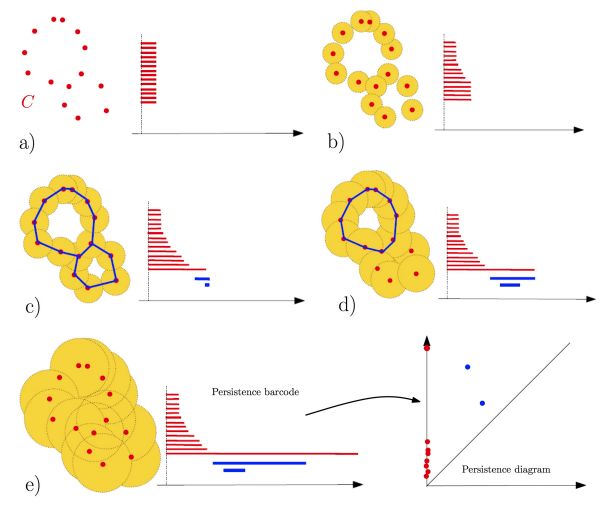
17/33Persistent homology
• How can we choose the right r ? We don’t have to choose!
• Persistent homology computes the homology of a sequence
of simplicial complexes:
Cechr1 (X ) ⊆ Cechr2 (X ) ⊆ Cechr3 (X ) ⊆ · · ·
• For very small r : β0 = n; βk = 0 for k ≤ 1
• For very large r : β0 = 1; βk = 0 for k ≤ 1
• We are looking for topological features that persist over long
ranges of r .
18/33Barcodes and diagrams
Figure 2: Chazal & Michel, Arxiv 2017 19/33Data analysis
• Split document-term matrix into 5 smaller matrices
• One for each leader
• Reduce dimension using PCA
• Compute persistent homology on reduced data
• Analysis conducted in Python using scikit-tda
20/33Persistence diagrams
21/33Bottleneck distance
Bottleneck distance to compare 0-th homology; visualize using
Multidimensional Scaling.
AS EM JS JT MB
AS 0.67 0.20 0.42 0.30
EM 0.67 0.56 0.39 0.78
JS 0.20 0.56 0.41 0.28
JT 0.42 0.39 0.41 0.39
MB 0.30 0.78 0.28 0.39
22/33Discussion
• The two most distant leaders are from the two smallest
parties (EM and MB)
• AS and JS have a similar goal: replacing JT. Could explain
why they are close.
• JS is closer to EM than MB, and the opposite is true for AS.
• In fact, by rotating the points, the x-axis could order the
leaders from left to right in the “expected” order.
23/33Discussion
• More generally, persistent homology can be used for feature
extraction in text data (Gholizadeh et al, 2020), document
clustering and classification (Guan et al, 2016).
• Persistence diagrams can be embedded in Hilbert spaces, and
therefore used with kernel methods for prediction
• It is also gaining popularity in other fields, e.g. social network
analysis (Almgren et al, 2017), change-point analysis
(Islambekov et al, 2019), understanding deep neural networks
(Gebhart et al, 2019)
24/33Mapper algorithm
• Data visualization for high-dimensional datasets
• Alternative to manifold learning and dimension reduction
• Main idea: Study the data by looking at its image under a
function f : Rp → R.
25/33Mapper algorithm
Algorithm
Input: A dataset X , a function f : Rp → R, a set U of intervals
covering the image f (X ).
• For each interval U ∈ U, cluster the pre-image f −1 (U).
• For each cluster, draw a node.
• Connect a pair of nodes if their corresponding clusters have a
non-trivial intersection.
Output: A graph (or network).
26/33Mapper algorithm
Figure 3: Chazal & Michel, Arxiv 2017
27/33Choice of f
• The Mapper algorithm requires the user to make a few
choices:
• Cover U
• Clustering algorithm
• Choosing the right function f can have a significant impact on
the resulting graph.
• Common choices include:
• Density function
• PCA (or manifold learning) coordinates
• Distance to a fixed point
28/33Data analysis
• Use the full document-term matrix
• Can we recover leaders/topics from Mapper graph?
• Choice of f : t-SNE coordinates
• For cover and clustering: use default from Kepler Mapper
library.
29/33Data analysis
30/33Discussion
• Unfortunately, not much to see here...
• However, Mapper has been very successful in the literature.
• Used for topic detection (Torres-Tramòn et al, 2015), Bitcoin
ransomware prediction (Akcora et al, 2019)
31/33Room for improvement
• Sparsity is a feature of text data, but it may be possible to
mitigate it via lemmatization.
• Use bootstrap on persistence diagrams.
• Tune dimension reduction steps and function in Mapper
32/33Future inquiries
• Impact of dimension reduction on TDA calculations
• How far can we push algorithms?
• Can we reconstruct the manifold? Where are the holes?
33/33Questions or comments?
For more information and updates, visit
maxturgeon.ca.
33/33You can also read