Is ENSO associated with Precipitation Patterns in Lake Valencia Venezuela?
←
→
Page content transcription
If your browser does not render page correctly, please read the page content below
Vol. 20 (2020): 75-87               ISSN 1578-8768
                                                                    ©Copyright of the authors of the article. Reproduction
                                                                  and diffusion is allowed by any means, provided it is done
                                                                    without economical benefit and respecting its integrity

                     Is ENSO associated with Precipitation Patterns
                            in Lake Valencia Venezuela?
                                José Hernández1 and Luis-Ángel Rodríguez2
              Departamento de Matemáticas, FACYT, Universidad de Carabobo, Venezuela.
                     1 , 2

                               (Received: 13-Aug-2020. Published: 28-Oct-2020)

Abstract
The objetive of this investigation is to determine if there exists an effect between El Niño phenomenon and the
rainfall in the Lake Valencia basin. The Standardized Precipitation Index (SPI), is used to measure the different
intensities of precipitation in the area of study. We implemented a Gaussian hidden Markov model (GHMM) to
describe the temporal evolution of each rainfall regime. Autoregressive models are implemented to describe the
monthly evolution of the different states of the Southern Oscilation Index (SOI) and the Multivariate ENSO Index
(MEI). Finally, the relationship between the Macroclimatic variables associated to the ENSO and the hydrome-
tereological variables associated to Lake Valencia basin, were caculated using the Pearson correlation coefficient
(r).

Key words: Lake Valencia, Hidden Markov model, Autoregressive with Markov Regime (AR-RM), Standardi-
zed Precipitation Index (SPI), Gaussian hidden Markov model (GHMM), Southern Oscillation Index (SOI) and
Multivariate ENSO Index (MEI).
Resumen
El objetivo de este trabajo es determinar si el fenómeno de El Niño influye o no en el régimen de precipitaciones de
la cuenca del Lago de Valencia. Las precipitaciones en el área de estudio son estandarizadas por intensidades uti-
lizando el índice SPI. Se implementa un modelo oculto de Markov Gaussiano para describir la evolución temporal
del régimen pluviomérico. Modelos Autorregresivos con régimen de Markov son implementados para describir las
distintas fases de los índices SOI y MEI. Finalmente, la relación entre las variables macroclimáticas asociadas
al ENSO y las variables meteorológicas en la cuenca del Lago de Valencia es medida a través del cálculo del
coeficiente de correlación de Pearson (r).

Palabras clave: Lago de Valencia, Modelo Oculto de Markov, Autorregresivos con régimen de Markov (AR-RM),
Standardized Precipitation Index (SPI), Modelo oculto de Markov Gaussiano (GHMM, siglas en inglés), Southern
Oscillation index (SOI) y Multivariate ENSO Index (MEI).

1. Introduction
The purpose of this work is to determine if there exists an effect of El Niño-Southern Oscillation (ENSO)
with precipitation patterns in Lake Valencia, Venezuela. For this, we study the rainfall in the Lake Valen-
cia basin and evolution of the different states of the Southern Oscilation index (SOI) and the Multivariate
ENSO Index (MEI; Wolter and Timlin, 1993). The Standardized Precipitation Index (SPI), is used to
measure the different intensities of rainfall data from a network of stations in Lake Valencia basin.
We fit Gaussian hidden Markov model (GHMM) to the SPI. This model provides a classification of
meteorological regime (weather type). Such models are used to model rainfall, the basic idea consists
of introducing an extra variable to describe the weather type, see Allard et al. (2015) and references. In
fact, characterizing the intensities that could produce floods is of great interest in the study of lakes that
76                            R EVISTA DE C LIMATOLOGÍA , VOL . 20 (2020)

are located near to populations. In Lake Valencia, floods have been reported in its southern zone. These
precipitations have caused disasters affecting the population and services, Arias et al. (2017).
The climatic phenomenon under study, ENSO, has two phases: the warm (El Niño) and the cold (La
Niña). These phases occur alternatively with neutral conditions. The intensity of the phenomenon is
usually measured using both the Multivariate ENSO index (MEI) and the Southern Oscillation Index
(SOI). We propose to use an autorregressive process with Markov regime (AR-RM) to fit ENSO index
and SOI index data. This modeling approach for this data type have been studied for example by Xuan
(2004) and Cárdenas-Gallo et al. (2015). Finally, the relationship between the macroclimatic variables
associated to the ENSO and the hydrometereological variables associated to the Lake Valencia basin
were caculated using the Pearson correlation coefficient (r).
This article is organized in seven main parts. In Section 2, we describe the data used for this work as well
as the preliminary treatments. Section 3 provides a model for the precipitation. We proceed with classic
time series analysis. Section 4 is devoted to calculating the SPI and using a Gaussian Hidden Markov
model for classifying the levels of intensity of the precipitations. The ENSO phases are modeled by an
AR-RM process in Section 5. A SAEM-type algorithm is used to estimate the parameters of process
AR-RM. In Section 6, we compare the rainfall regime and the ENSO phenomenon. We carry out the
comparison by calculating the correlation between the two series. Finally, Section 7 is devoted to the
conclusion.

2. Data description
Lake Valencia 2943 km2 basin lies between the Aragua Valley and Carabobo state at an elevation of
420 m asl, see Figure 1. This lake, also known as Tacarigua, is the largest endorheic freshwater body in
Venezuela (Díaz et al., 2010). Lake Valencia occupies a tectonic depression called Graben de Valencia,
between the Cordillera de la Costa, at the north, and the Serranía del Interior, at the south. The body
of the water of lake has a volume of 6.30 km3 , an average depth of 18 m, and maximum depth of 39 m
approximately. There are 18 sub-basins taxing in the lake (Trejo et al., 2015).

                        Fig. 1: Map of the studied area. (Source: Google maps.)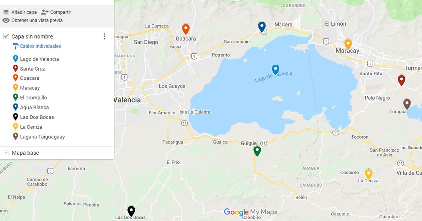
R EVISTA DE C LIMATOLOGÍA , VOL . 20 (2020)                                 77

The database used for this article was provided by the Instituto Nacional de Meteorología e Hidrología
(INAMEH). We used a small network of J = 8 rainfall stations located in the Lake Valencia basin. These
stations represent a good spatial coverage across the region under study. The weather stations names,
geographical positions and number of observed years are shown in Table 1.
The calculation of SPI requires that there are no missing data in the time series. Additionally, the data
record length must be at least 30 years, according to the World Meteorological Organization (McKee et
al., 2012). The amount of precipitation was evaluated with regard to the monthly arithmetic means of
daily precipitation. In this work we complete the data of missing periods by using a moving average
process of order 3.

                              Table 1: Weather stations and years observed.

   Station         Locality                    Coordinates                         Years
    code            name               Lat        Long     Height      Period      Missing     Observed
    417          Santa Cruz           10,167    -67,488     444      1966-1999       3           30
    452            Guacara            10,236    -67,884     300      1949-1993       1           43
    466           Maracay             10,25      -67,65     436      1934-1992       0           58
    488      Colonia El Trompillo     10,061    -67,772     450      1960-1993       0           35
    489         Agua Blanca           10,046    -67,838     515      1951-2005       3           68
    491        Las Dos Bocas          9,961     -67,995     550      1949-2005       4           52
    497          Las Cenizas          10,027    -67,599     670      1960-2003       3           43
    1494     Embalse Taiguaiguay      10,147      -67,5     438      1951-1999       3           45

We used the ENSO index series data as reported by the National Oceanic and Atmospheric Administra-
tion (NOAA) on its World Wide site. We considered the SOI index and the MEI index over the period
1951-2017.

3. Precipitation Modeling
Let Yt ( j) represent the observed precipitation amount on time t at station j = 1, . . . , 8. We will model
Yt ( j) as a random variable. We proceed with a classic time series analysis. First, the stationarity and
stationality of the precipitation series were analyzed by the autocorrelation function and partial autocor-
relation function methods. We investigated the series of the rainfall at each station. See Figure 2 for
an example of such data series. The autocorrelation and the partial autocorrelation obtained indicated
stationarity, as it is illustrated in Figure 3.

                       Fig. 2: Precipitation time series from station Agua Blanca.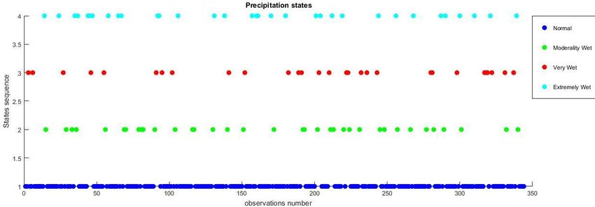
78                          R EVISTA DE C LIMATOLOGÍA , VOL . 20 (2020)

       Fig.3: Autocorrelation (top) and partial autocorrelation (bottom) at Agua Blanca station.

Indeed, we distinguished two seasons, one dry and one wet. The graph of monthly averages shows
that the months of January, February, March, April and December are the months of the lowest rainfall
amounts. While the months between May and November are the months with the highest amount of
rainfall (Figure 4).

                            Fig. 4: Monthly average of rainfall by locality.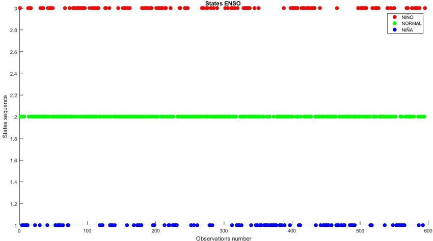
R EVISTA DE C LIMATOLOGÍA , VOL . 20 (2020)                                 79

The partial correlation converges to 0, which is an indicative of stationarity. But, the tendency of the
series is not clear. It is known, in the case of the autorregresive process with order p, (AR(p)), that
we can study the stationarity by considering the associated characteristic polynomial, see Fermín et al.
(2016). The test Dickey-Fuller, is used as an indicative of the stationarity. If the p-value is lower than
the established α = 0, 05 level of confidence, the null hypothesis of a unit root is rejected. The result was
that all stations are stationary with a p-value of 0.001 or lower.
Observing in the series of precipitation the maximums, minimums and averages values at each station, we
obtain an indicative of the level of precipitation. The Table 2 shows the minimum and maximum rainfall
(abbreviated as min ppn and max ppn, respectively) for each station in the study area. We computed the
SPI to obtain a classification of the intensity levels of the series. We needed to complete the missing
data, see Table 3. We adjust a moving average process of order 3 to the data. In this way, we completed
and smoothed the data. Then we proceeded to calculate the SPI, using the ’spi’ library of the statistical
package R, see Neves (2015).

                Tabla 2: Maximum and mininimum recorded precipitation at the stations.

                    Locality            Period-years    Minimum (mm)        Maximum (mm)
                  Santa Cruz             1966-1999            0                  351
                    Guacara              1949-1993            0                 419,9
                   Maracay               1934-1992            0                  454
              Colonia El Trompillo       1960-1993            0                 311,7
                 Agua Blanca             1951-2005            0                 633,6
                Las Dos Bocas            1949-2005            0                 475,5
                  Las Cenizas            1960-2003            0                 446,6
              Embalse Taiguaiguay        1951-1999            0                 334,6

4. A Gaussian Hidden Markov model for SPI
In this section we calculate the SPI index, after using the Gaussian hidden Markov Model, intensity levels
are classified. The SPI classification scheme used is

      ’EW’=Extremely Wet

      ’VW’=Very Wet

      ’MW’=Moderality Wet

      ’N’=Normal

      ’MD’=Moderality Dry

      ’VD’=Very Dry

      ’ED’=Extremely Dry

For each locality under study in Table 3, we classify the intensities according to the previous scheme,
writing in the table Yes or NO if there was an occurrence. We observe in this table that 100 % of the
locations have intensity level precipitation of the type (EW, VW, MW, N). While 62.50 % presented a
moderately dry intensity (MD) and only 12.50 % presented a very dry precipitation (VD). Special focus
was made on the intensities (EW, VW, MW, N).
80 R EVISTA DE C LIMATOLOGÍA , VOL . 20 (2020)
Table 3: Intensity Levels at the stations.
Localidad EW VW MW N MD VD ED
Santa Cruz Yes Yes Yes Yes Yes NO NO
Guacara Yes Yes Yes Yes NO NO NO
Maracay Yes Yes Yes Yes Yes NO NO
Colonia El Trompillo Yes Yes Yes Yes Yes NO NO
Agua Blanca Yes Yes Yes Yes Yes NO NO
Las Dos Bocas Yes Yes Yes Yes NO NO NO
Las Cenizas Yes Yes Yes Yes Yes Yes NO
Embalse Taiguaiguay Yes Yes Yes Yes NO NO NO
Let Zt ( j) be the SPI index value on time t at station j = 1, . . . , 8. In the following expresion, the index j
that indicates the station is omitted, with the purpose of simplifying the notation. The GHMM is defined
by
Zt = µXt + σXt et (1)
where {Xt }t≥0 is a homogeneous discrete Markov chain, the space state is the discrete set {1, . . . , m}.
Assume that {et } is a Gaussian standard independent observation. The unknown paramaters are the
intensity levels µi , the noisy variance σ2i in each regime, with i = 1, . . . , m, as well as the state transition
probability distribution A = {ai j }, with transition probability defined by ai j = P(Xt = j|Xt−1 = i), i, j =
1, . . . , m.
We assume that m is known. In fact, the previous analysis, done using the SPI, leads us to consider
m = 4, then µi ∈ {N, MW,VW, EW }, i = 1, . . . , 4. Hence, the parameters to be estimated are,
Ψ = (A, µ1 , . . . , µ4 , σ1 , . . . , σ4 ).
To estimate Ψ, we considered the maximum likelihood estimator. The log-likelihood of the model can
be written in the following form:
T
L(Ψ) = ∑ ∑ log ψ(Zt − µxt , σxt )axt ,xt−1 πxt
X1:T =x1:T t=1
where ψ(x, v) is a density N (0, v2 ). The log-likelihood estimator of L(Ψ) is a root of the equation
∇L(Ψ) = 0. The solution of this equation can be computed efficiently with an EM algorithm, see Fermín
et al. (2016) and its references. The EM algorithm is divided into two stages: the expectation stage (E)
and the maximization stage (M). In the step E, we calculate the expectation of the log-likelihood of the
complete data conditioned on the observed data. In the next step M, this function is maximized. This
procedure is repeated iteratively.
In order to illustrate the results when modeling the SPI with a GHMM, we chose the Trompillo locality.
This station has the shortest historical period and more Extremely Wet (EW) rainfall was recorded. This
locality will be representative when calculating the correlation with the ENSO events.
The results of estimation by means of the EM procedure in Trompillo station are: transition matrix,
0, 8875 0, 08571429 0, 01071429 0, 01607143
0, 76666667 0, 11666667 0, 06666667 0, 05
 =
0, 54545455
0, 27272727 0, 09090909 0, 09090909
0, 84615385 0, 15384615 0 0R EVISTA DE C LIMATOLOGÍA , VOL . 20 (2020) 81
intensity levels µ and variance σ2 ,
0.064991721582782 0.064991721582780
1.237921717425580 0.000000000000002
µ̂ =
1.859111513498231 σˆ2 =
0.000000000000004
2.200000000000000 0
The Figure 5 shows the percentages of the precipitation states of the Trompillo locality. It was observed
that more than 8.3544 % of rainfall were Extremely Wet (EW), 7.3417 % were Very Wet (VW), 9.1139
% MW (MW), 12.92 % of moderately dry intensity (MD) and the 62.27 % were rainfall with normal
intensities (N).
Fig. 5: Intensity levels at the Trompillo station.
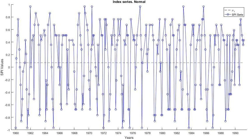
We build a plot with the classified precipitation series according to their levels. This allows us to have a
complete idea of the intensities, in a single graphic representation (Figure 6).
Fig. 6: Intensity levels and clasification of rainfall at the Trompillo station.82 R EVISTA DE C LIMATOLOGÍA , VOL . 20 (2020)
Now, we consider to separate the models for each intensity level, in the equation (1) the state is fixed,
Zt = µi + σi et (2)
for i = 1, . . . , 4. We represent each equation separately. This allows us to observe how each state of
precipitation evolves over time, without having to study all precipitation phases simultaneously. The
results are shown in Figure 7. The advantages of applying the models (GHMM) over the index under
study (SPI) are shown.
a b
c d
Fig. 7: SPI series states: Normal (a); Moderately Wet (b); Very Wet (c); Extremely Wet (d).
5. AR-RM for SOI
ENSO is a cyclical phenomenon in which it is possible to identify two regimes over time (La Niña and El
Niño). The behavior patterns during each of the two phases are opposite and differentiable. On the other
hand, the duration and the change between regimes is variable over time. These types of models for the
ENSO phenomenon have been used for example by Xuan (2004) and Cárdenas-Gallo et al. (2015).
An autorregressive process with Markov Regime is defined for the SOI by
Yt = ρXt Yt−1 + bXt + σXt et (3)
where {Xt }t≥0 is a homogeneous discrete Markov chain, the space state is the discrete set {1, . . . , m}.
Assume that {et } is a Gaussian standard independent observation. The unknown parameters are the ρi ,
bi , the noisy variance σ2i in each regime, with i = 1, . . . , m, as well as the state transition probability
distribution A = {ai j }, with transition probability defined by ai j = P(Xt = j|Xt−1 = i), i, j = 1, . . . , m.
We assume that the state number is m = 3. We consider three states Xt , since ENSO is divided in three
phases: El Niño, La Niña, and the transition state we call Normal.R EVISTA DE C LIMATOLOGÍA , VOL . 20 (2020) 83
Hence, the parameters to be estimated are,
Ψ = (A, ρ1 , ρ2 , ρ3 , b1 , b2 , b3 , σ1 , σ2 , σ3 ).
To estimate Ψ, we considered the maximum likelihood estimator. The log-likelihood of the model can
be written in the following form:
T
L(Ψ) = ∑ ∑ log ψ(Zt − ρxt − bxt , σxt )axt ,xt−1 πxt
X1:T =x1:T t=1
where ψ(x, v) is a density N (0, v2 ). The log-likelihood estimator of L(Ψ) is a root of the equation
∇L(Ψ) = 0. In order to avoid local minima in the solution of this equation, we have used a stochastic
approximation of the EM algorithm, the SAEM algorithm, see Fermín et al. (2016) and its references.
The E stage in the algorithm EM is replaced by a simulation stage and an approximation procedure.
The results when modeling the SOI with an AR-RM. The parameters estimated are the transition matrix,
the slope,
0.4274 0.4597 0.1129 −0.7113
 = 0.1976 0.5836 0.2188 b̂ = 0.0237
0.0426 0.5674 0.3901 0.7486
the variance, and the intercept
0.998952924206662 0.98520
σˆ2 = 0.968681703610350 ρ̂ = −0.472054506176259
0.602621116771551 0.7486
In the 1951-2017 period, 20.84% of El Niño events were observed, 54.45% normal periods and 23.86%
of La Niña phenomenon. A graphic representation of these results are shown in Figure 8.
6. Correlation
In this section, we analyze if there is a correlation between the rainfall regime and the ENSO phe-
nomenon. Recall that the climate regime was classified by intensities through the SPI index denoted by
Zt . While ENSO occurrences are characterized by the SOI index denoted by Yt . In Table 4 we show the
results. For the calculation, only the months with intensities EW and MW and with the presence of the
El Niño phenomenon were considered.
Table 4: Correlation between SPI and SOI.
Locality Time period Correlation
Santa Cruz 1966-1999 -0,1580
Guacara 1951-1993 0,0463
Maracay 1951-1992 -0,13285057
Colonia el Trompillo 1960-1993 -0,02018438
Agua Blanca 1951-2005 0,0716
Las Dos Bocas 1951-2005 -0,0475
Las Cenizas 1960-2003 -0,11028861
Embalse de Taiguaiguay 1951-1999 -0,0288111484 R EVISTA DE C LIMATOLOGÍA , VOL . 20 (2020)
Fig. 8: States (top) and classified (bottom) SOI series.
The statistical significance of the correlation between the phenomena is measured by calculating the
Pearson test. The correlation coefficients were computed using the MATLAB software, in particular
the command “corrcoef”. The results displayed in Table 5 show that in 7 of the 8 locations there is no
correlation between the SOI and the MEI index.
Table 5: Pearson test with level of confidence α = 0.05.
Locality p-value (SOI) p-value (MEI)
Santa Cruz 0,0022 0,2194
Guacara 0,2994 0,2994
Maracay 0,0028 0,8668
Colonia El trompillo 0,8596 0,9362
Agua Blanca 0,1043 0,0908
Las dos Bocas 0,2600 0,0002
Las Cenizas 0,0156 0,1483
Embalse Taiguaiguay 0,5089 0,1520R EVISTA DE C LIMATOLOGÍA , VOL . 20 (2020) 85
The ENSO phases calculated with the SOI index, can be visualized for each state by considering equation
3 separately for i = 1, 2, 3
Yt = ρiYt−1 + bi + σi et ,
Figure 9 shows the results.
a b
c
Fig. 9: ENSO phases: El Niño (a); Normal (b); La Niña (c).
In 5 of the 8 localities, the null correlation hypothesis is rejected. Therefore in these locations there is no
evidence of an interrelation between the two phenomena.
In order to corroborate the results obtained, the experiments were repeated considering the MEI index
for the ENSO phenomenon. In Table 6 the calculation of the correlation taking the values of the MEI are
shown.
Table 6: Correlation between the SPI and the MEI.
Locality Time period Correlation
Santa Cruz 1979-1999 -0,1182
Guacara 1979-1993 0,1351
Maracay 1979-1992 -0,0130
Colonia el Trompillo 1979-1993 -0,0649
Agua Blanca 1979-2005 0,1217
Las Dos Bocas 1979-2005 -0,2298
Las Cenizas 1979-2003 -0,1298
Embalse de Taiguaiguay 1979-1999 0,0678
Table 7 shows the coincidences in dates of the Extremely Wet rainfall with the ENSO stations in the
Colonia el Trompillo locality. We observe that precipitation with Extremely Wet intensity occurs on
15.15% of the months where El Niño events occurred, while La Niña events occurred in 21.21% stations
and 63.63% were normal events.86 R EVISTA DE C LIMATOLOGÍA , VOL . 20 (2020)
Table 7: ENSO phases at extremely wet months in the Colonia el Trompillo station.
Month ENSO Month ENSO Month ENSO
Jul-1960 Niña Aug-1969 Normal Jul-1980 Niño
May-1962 Niño Sep-1970 Normal Apr-1981 Niño
Jul-1963 Normal Oct-1972 Normal Jun-1983 Normal
Sep-1963 Normal Jun-1973 Niña Jul-1984 Niña
Jun-1964 Niña May-1975 Normal Aug-1985 Niña
Jul-1964 Normal Aug-1975 Normal May-1987 Normal
Sep-1964 Normal Sep-1975 Normal Aug-1987 Normal
Sep-1965 Normal Jul-1976 Normal Aug-1988 Niño
Jun-1966 Normal Jun-1977 Normal Sep-1989 Niño
Aug-1966 Niña Jun-1979 Normal Sep-1990 Normal
Jul-1969 Normal Sep-1979 Niña Jul-1992 Normal
7. Conclusion
From the results of the data analysis, we could see that rainfall shows a seasonal behavior. The months of
precipitation in the lake basin show a unimodal distribution with two periods clearly differentiated, one
period is characterized by above average rainfall, and occurs between May and October; the rainfall in
the other period is below average, ocurring between November and April. The maximum rainfall value
is presented in August and the minimum in March. The intensities, in the area of study, were classified
as normal, moderately wet, very wet and extremely wet. Dry periods were recorded but only in 50 %
of the localities, the most observed rainfall intensity is normal. This is one of the indicators taken into
account that shows the presence of the phenomenon, since in the entire series of precipitation there were
occurrences of very wet and extremely wet intensities. These occurrences were less than 7.3417 % and
also 9.1139 % respectively.
On the other hand, the previous analysis does not guarantee that the phenomenom is present or not.
The contribution of the models with hidden variables allowed us to study individually each phase of the
ENSO and rainfall, as well as its temporal evolution. We observed that the occurrences of El Niño were
20.84 % throughout the period of study. Likewise in the locality El Trompillo, used as a reference for
the other localities in the Extremely Humid precipitation series, there were coincidences with the dates
only 15.15 % of the time.
The analysis of the correlation between the ENSO phenomenon and rainfall patterns in most places,
shows us that for the data studied there is no statistical evidence revealing a correlation of rainfall patterns
in the basin of Lake Valencia and the ENSO. This could be due to the fact that there exists a marked
microoclimate behavior in this basin.
Acknowledgments
We thank the editor, José Guijarro, and anonymous referees for their insightful comments that greatly
contributed to the improvement of this article.
J. Hernández is thankful to Instituto Nacional de Meteorología e Hidrología(INAMEH) by data provided.
References
Allard D, Ailliot P, Monbet V, Naveau P (2015): Stochastic weather generators: an overview of weather
type models. Journal de la Société Française de Statistique, 156:101-113.
Arias A, Sáez V, Siso E (2017): Inundaciones ocurridas entre 1970 y 2005 y su relación con la precipi-
tación del percentil 25 %. Región Central de Venezuela. Terra Nueva Etapa, 53:33–48.R EVISTA DE C LIMATOLOGÍA , VOL . 20 (2020) 87 Cárdenas-Gallo I, Akhavan-Tabatabaei R, Sánchez-Silva M, Emilio Bastidas-Arteaga (2015): A Markov regime-switching framework to forecast El Niño Southern Oscillation patterns. Natural Hazards, 81:829- 843. Díaz E, Pérez R, Armas M (2010): Propuesta de los actores claves del plan de educación ambiental en la cuenca del lago de Valencia. Observatorio laboral revista Venezolana, 3:43–59. Fermín L, Rodríguez LA, Ríos R (2016): Modelos de Markov Ocultos. XXIX Escuela Venezolana de Matemáticas, EMALCA-Venezuela, Mérida, Venezuela. Neves J (2015): Compute the SPI index using R. https://cran.r-project.org/package=spi McKee TB, Doesken NJ, Kleist J (2012): Índice normalizado de precipitación. Guía del usuario. Orga- nización Meteorológica Mundial, Ginebra, Suiza. SOI. Indice de Oscilación del Sur. National Centers For Evironmental Information. https://www.ncdc. noaa.gov/teleconnections/enso/indicators/soi/ Trejo P, Guevara Pérez E, Barbosa Alves H, Uzcátegui Briceño C (2015): Tendencia de la precipitación estacional e influencia de el niño – ocilación austral sobre la ocurrencia de extremos pluviométricos en la cuenca del lago de Valencia-Venezuela. Tecnología y ciencias del agua, 6:33-48. Wolter K, Timlin MS (1993): Monitoring ENSO in COADS with a seasonally adjusted principal compo- nent index. In: Proceedings of the 17th Climate Diagnostic Workshop, Norman, Oklahoma, pp. 52-57. Xuan T (2004): Autoregressive Hidden Markov Model with Application in an El Niño Study. University of Saskatchewan Saskatoon.
88 R EVISTA DE C LIMATOLOGÍA , VOL . 20 (2020)
You can also read