It is time to mate: population-level plasticity of wild boar reproductive timing and synchrony in a changing environment
←
→
Page content transcription
If your browser does not render page correctly, please read the page content below
Current Zoology, 2021, 1–9
                                                                                                                     doi: 10.1093/cz/zoab077
                                                                                       Advance Access Publication Date: 17 September 2021
                                                                                                                            Original Article

Original Article

It is time to mate: population-level plasticity of

                                                                                                                                                                          Downloaded from https://academic.oup.com/cz/advance-article/doi/10.1093/cz/zoab077/6371954 by guest on 06 November 2021
wild boar reproductive timing and synchrony in
a changing environment
Rudy BROGI * , Enrico MERLI, Stefano GRIGNOLIO                                                        , Roberta CHIRICHELLA,
Elisa BOTTERO, and Marco APOLLONIO
Department of Veterinary Medicine, University of Sassari, via Vienna 2, Sassari I-07100, Italy
*Address correspondence to Rudy Brogi. E-mail: r.brogi@studenti.uniss.it

Handling editor: Zhi-Yun Jia (                 )
Received on 5 June 2021; accepted on 13 September 2021

Abstract
On a population level, individual plasticity in reproductive phenology can provoke either anticipa-
tions or delays in the average reproductive timing in response to environmental changes.
However, a rigid reliance on photoperiodism can constraint such plastic responses in populations
inhabiting temperate latitudes. The regulation of breeding season length may represent a further
tool for populations facing changing environments. Nonetheless, this skill was reported only for
equatorial, nonphotoperiodic populations. Our goal was to evaluate whether species living in tem-
perate regions and relying on photoperiodism to trigger their reproduction may also be able to
regulate breeding season length. During 10 years, we collected 2,500 female reproductive traits of
a mammal model species (wild boar Sus scrofa) and applied a novel analytical approach to repro-
ductive patterns in order to observe population-level variations of reproductive timing and syn-
chrony under different weather and resources availability conditions. Under favorable conditions,
breeding seasons were anticipated and population synchrony increased (i.e., shorter breeding sea-
sons). Conversely, poor conditions induced delayed and less synchronous (i.e., longer) breeding
seasons. The potential to regulate breeding season length depending on environmental conditions
may entail a high resilience of the population reproductive patterns against environmental
changes, as highlighted by the fact that almost all mature females were reproductive every year.

Key words: breeding season length, phenology, photoperiodism, population ecology, reproduction, wild boar.

Animals face changing environments throughout their whole life                             tool to deal with such irregular and unpredictable changes on a
cycles. Individuals are adapted to the changes that are regular and                        population level (Hertel et al. 2020).
predictable. The most common example is seasonality in temperate                               A plastic reproductive phenology is a key ecological determinant
zones, for which photoperiod variation over the year represents a re-                      of animal population sensitivity to changing environments as it rep-
liable and easily accessible predictor (Bradshaw and Holzapfel                             resents the time dimension-linkage between reproduction and envir-
2007). Other phenomena arise with irregular and usually unpredict-                         onment (Post et al. 2008; Ogutu et al. 2015). Such plasticity takes
able patterns, such as interannual weather variability and food or                         effect on several levels (ovulation, conception, and birth) on both
prey availability (e.g., fruit mast years) related to it (Nussbaumer et                    individuals (Canu et al. 2015) and populations (Fernández et al.
al. 2018). Whereas it is known that individuals and populations                            2020). However, it is generally constrained by the reliance on rigid
may react with plastic responses (e.g., Ruf et al. 2006; Ogutu et al.                      reproductive cues (i.e., photoperiod variations throughout the year,
2015), inter-individual phenotypic diversity may represent a further                       Bradshaw and Holzapfel 2007) that do not depend on the

C The Author(s) (2021). Published by Oxford University Press on behalf of Editorial Office, Current Zoology.
V                                                                                                                                                                    1
This is an Open Access article distributed under the terms of the Creative Commons Attribution-NonCommercial License (https://creativecommons.org/licenses/by-nc/4.0/),
which permits non-commercial re-use, distribution, and reproduction in any medium, provided the original work is properly cited. For commercial re-use, please contact
journals.permissions@oup.com
2                                                                                                         Current Zoology, 2021, Vol. 0, No. 0

environmental conditions. Most ungulate populations, or at least           seasons (Santos et al. 2006; Canu et al. 2015). The reproductive out-
those living at latitudes with clear day length variations throughout      put of this species was widely investigated thanks to the large
the year, typically show a tight reliance on photoperiod to trigger        amount of data regarding culled individuals provided by hunting
their reproduction (Zerbe et al. 2012). Nevertheless, evidence that        activities (e.g., Servanty et al. 2009; Fonseca et al. 2011; Canu et al.
favorable environmental and nutritional conditions facilitate a            2015; Bergqvist et al. 2018; Touzot et al. 2020). A high degree of in-
slightly earlier reproduction was frequently reported even in species      dividual plasticity was reported for several reproductive parameters
whose predominant cue is photoperiodism (McGinnes and Downing              of wild boar females, including their reproductive phenology, which
1977; Hamilton and Blaxter 1980; Flydal and Reimers 2002;                  tends to be anticipated in response to good environmental condi-
Wolcott et al. 2015). Thus, a certain degree of plasticity in the repro-   tions (e.g., Servanty et al. 2009; Canu et al. 2015). Nevertheless, so
ductive timing (hereafter RT, always referred to the population            far, the relationship between environmental drivers and population

                                                                                                                                                      Downloaded from https://academic.oup.com/cz/advance-article/doi/10.1093/cz/zoab077/6371954 by guest on 06 November 2021
level) seems to be quite spread among ungulate species and this can        RT and RS has never been evaluated.
be expected to produce temporal displacements of breeding seasons              In this study, we aimed to evaluate age-specific wild boar popu-
among different years. In this context, the most plastic species have      lation responses to such environmental factors as weather and
a reproductive output which is less constrained by environment, as         resources availability in terms of both RT (anticipated or delayed
they can respond to negative conditions by delaying the breeding           breeding seasons) and RS (longer or shorter breeding seasons). In so
season (Servanty et al. 2009).                                             doing, we aimed to determine whether:
     The phenotypic diversity of reproductive phenology within a
population (namely, “reproductive synchrony,” Findlay and Cooke              i. wild boar shows an interannual variability of both population
1982, hereafter RS) directly affects breeding (and, consequently,               RT and, though inhabiting temperate regions, RS;
birth) season length. Higher RS (i.e., shorter breeding seasons) was        ii. such interannual variability is the result of modifications of the
observed in ungulate species and populations living in more seasonal            overall individual likelihood of ovulating and getting pregnant,
and constant environments (English et al. 2012; Zerbe et al. 2012),             which in turn is affected by a number of environmental factors
relying on more specialist foraging strategies (English et al. 2012),           directly or indirectly related to resources availability; and
showing gregarious habits associated with precocial young (Sinclair        iii. such environmental factors influence the population RT and
et al. 2000) and an even, rather than female-biased, sex ratio of               RS.
adults (Milner et al. 2007). In a number of equatorial savanna ungu-
lates, a substantial interannual RS variability in response to environ-    Materials and Methods
mental conditions was reported, with longer breeding seasons
observed during drought years (Ogutu et al. 2010, 2014). This phe-         Study area
nomenon comes as no surprise in species mainly relying on environ-         We collected data in a mountainous area of 13,400 ha in Central
mental cues (i.e., rainfall patterns) to time their reproduction           Italy (Northern Apennines, Italy, 43 480 N, 11 490 E), which
through a nutritional status mediation (Ogutu et al. 2015).                includes 2,700 ha of protected area (Oasi Alpe di Catenaia). Lowest
Conversely, environment-driven interannual RS variability in ungu-         and highest altitudes reach 330 and 1,414 m above the sea level, re-
lates of temperate regions (i.e., relying on photoperiod variations,       spectively. The climate is temperate continental with a marked sea-
Zerbe et al. 2012) is not obvious and so far has never been reported.      sonality. A mean temperature of 18.7  C and a daily precipitation of
On the one hand, as photoperiodism follows genetic heritability            1.73 mm are recorded in summer, whereas winters are cold (mean
(Bradshaw and Holzapfel 2007; Zerbe et al. 2012), we may expect            temperature of 1.2  C) and rainy (daily precipitation of 3.55 mm).
RS degree to remain substantially constant under different environ-        Snowfalls are sporadic in winter and can also occasionally occur in
mental conditions, at least assuming that they homogeneously affect        spring. Mixed deciduous woods are the prevailing habitat category
all individuals. In this respect, Zerbe et al. (2012) reported unaltered   (67% of the total surface) and are mainly composed of Turkey oak
RS between wild ungulates and those kept in captive conditions             Quercus cerris, beech Fagus sylvatica, and chestnut Castanea sativa.
with high resources availability. On the other hand, resource-poor         Agricultural crops (16%), mixed open-shrubs areas (10%), and
years may provoke a higher inter-individual variability in the time        conifer woods (7%) cover the rest of the surface. In the surroundings
needed to achieve the nutritional condition required to reproduce          of the protected area, wild boar is unselectively hunted in drive
and ultimately reduce RS.                                                  hunts by teams of 25–50 people. During the study period, drive
     The simpler method to investigate the variability of both RT and      hunting was generally permitted 3 times a week from September to
RS on a population level is to compare the temporal occurrence and         January, with an average of 58.3 hunting days per year. As a yearly
duration of an adequate number of breeding seasons with one or             average of 6.4 wild boar/km2 was harvested, the population under-
more environmental variables (Ogutu et al. 2010, 2014; Fernández          went a high, but relatively constant, hunting pressure (Merli et al.
et al. 2020). Unfortunately, this approach requires the condensation       2017).
of large datasets into 1 observation per year, with a substantial loss
of statistical power. To overcome this limitation, analytical strat-       Data collection
egies aimed at evaluating the temporal variability of the individual       We collected and examined reproductive traits of 2,500 female wild
reproductive status with respect to certain environmental conditions       boars culled from 1 September to 31 January during 10 consecutive
should be applied. A further constraint for specific investigations of     hunting seasons (2006–2016). Culling date and live body mass were
RS variability in response to environmental changes is the typically       recorded for each individual. In so doing, we included the reproduct-
short breeding season of mammal populations inhabiting temperate           ive trait mass, though it accounted only for a negligible percentage
regions (Garel et al. 2009; Mason et al. 2011). We thus chose wild         of female live body mass (Brogi et al. 2021). All females were aged
boar (Sus scrofa) as a model species because it presents the rare con-     on the basis of their tooth eruption and abrasion (Briedermann
dition of living in temperate regions (i.e., in highly seasonal environ-   1990) and assigned to one of the following age classes: juvenile
ments) and, at the same time, showing relatively long breeding             (< 1 year), subadult (between 1 and 2 years), and adult (> 2 years).
Brogi et al. Population-level plasticity of wild boar reproductive timing and synchrony 3
In order to determine their reproductive status, we dissected ovaries Step 2: factors influencing individual reproductive status
and uterus of each female to check for the presence of corpora lutea After the analysis to test potential differences among seasons within
and embryos/fetuses, respectively. Corpora lutea were used as a sign age classes, we aimed to identify internal and external factors which
that ovulation occurred, whereas embryos and fetuses as a sign of influenced ovulation and pregnancy ratios. We modeled the individ-
ongoing pregnancy (e.g., Malmsten et al. 2017a). Over 823 culled ual likelihood of ovulating and, alternatively, of getting pregnant by
juvenile females, only 30 ovulated and 3 pregnant individuals were means of 4 GLMs with a binomial distribution (ovulation in suba-
identified. We thus decided to exclude the individuals belonging to dults, ovulation in adults, pregnancy in subadults, and pregnancy in
this class from our analysis. The Regional Hydrological Service of adults). The standardized culling date (days from 1 September) was
Tuscany kindly provided weather data (average temperature and used as predictor to consider photoperiod-mediated seasonal varia-
rain) daily recorded in a weather station located inside our study tions of the individual reproductive status. We also included such in-
Downloaded from https://academic.oup.com/cz/advance-article/doi/10.1093/cz/zoab077/6371954 by guest on 06 November 2021
area (43 420 N, 11 550 E). We obtained local data on yearly seed ternal factors as individual age (months) and live body mass (kg) as
productivity of beech, chestnut, and Turkey oak measured inside the predictors. Among external factors, 4 season average temperature
Oasi Alpe di Catenaia from an online database (Chianucci et al. and rain precipitation calculated on a yearly basis were used as pre-
2019) and used it as a measure of food availability. dictors to account for the potential effect of weather. Because all
individuals were culled between September of year x and January of
Data analysis year x þ 1, winter weather variables were averaged from December
Step 1: ovulation and pregnancy heterogeneity among years and of year x1 to February of year x, spring ones from March to May
classes of year x, summer ones from June to August of year x, and autumn
In order to assess interannual heterogeneity in ovulation and preg- ones from September to November of year x. Moreover, we used
nancy patterns, we modeled both individual likelihood of ovulating current year seed productivity of Turkey oak, beech, and chestnut
and getting pregnant throughout the sampling period. We divided (t/ha) measured on a yearly basis to check for potential effects of
our dataset into 2 sub-datasets corresponding to subadult and adult food availability on ovulation and pregnancy patterns. To summarize
females. By means of the glm() function of the stats package (R ver- the influence of the 3 deciduous species in a single variable, we
sion 4.0.3, R Development Core Team, 2015) we ran a Generalized included a further global forest productivity index in the models,
Linear Model (GLM) with a binomial distribution, with the individ- which we calculated following the protocol described by Bisi et al.
ual reproductive states (ovulated or pregnant, alternatively) as bin- (2018). Finally, we calculated the yearly average number of adult
ary-dependent variables, separately for the subadult and the adult males per female as the number of culled adult males (>3 years; Brogi
female sub-datasets. The binary variable “ovulated” took the value et al. 2021) divided by the total number of adult and subadult
1 whenever at least 1 corpus luteum, embryo, or fetus was detected, females. We added this yearly variable as a predictor within our mod-
and 0 otherwise; the binary variable “pregnant” took the value 1 els to take into account the potential effects of reproductive male rela-
whenever at least 1 embryo or fetus was detected, and 0 otherwise. tive abundance on female reproductive status (Milner et al. 2007).
In so doing, we built a total of 4 models, hereafter called “1S-ov” We recognize that, by measuring adult male availability on the basis
(model of ovulation in subadults), “1A-ov” (ovulation in adults), of culling data, we may obtain an unreliable approximation of the
“1S-pr” (pregnancy in subadults), and “1A-pr” (pregnancy in real population structure. However, in this study, we were only inter-
adults). We included in all models the interaction term between the ested in the variation of male availability throughout different years.
standardized culling date (expressed as days from 1 September) and Separately for each sub-dataset, we screened all available predic-
the hunting season (categorical) as the only predictor to check for tors for collinearity and multicollinearity by means of a Pearson cor-
interannual variations in the effect of the standardized date. The relation matrix (rp) and the variance inflation factor (VIF), setting
hunting season was expressed as a sequential number from 1 (refer- thresholds to rp ¼ 6 0.7 and VIF ¼ 3, respectively (Zuur et al. 2009).
ring to the 2006–2007 hunting season) to 10 (2015–2016). Weather variables of the same season (particularly spring and au-
To check for statistical differences among age classes in ovula- tumn) were the most recurring pairs of collinear variables. We per-
tion RT and RS, we used the models 1S-ov and 1A-ov to predict formed a random forest calculation (random.Forest package) to
yearly dates of onset, middle point, and end of ovulation on a popu- rank all predictors on the basis of their potential to explain the de-
lation level for each monitored hunting season. The dates in which pendent variable (Breiman 2001). The worst predictor variable of
the proportion of ovulated females reached 0.025, 0.5, and 0.975 each collinearity and multicollinearity condition was dropped until
were used as onset, middle point (inflection point of the curve) and all rp and VIF were below the corresponding thresholds. Finally, we
end date, respectively. In so doing, we included 95% of the pre- included the remaining predictor variables in a full GLM and used
dicted ovulation events between the onset and end dates. In order to the dredge() function (MuMln package) to run a set of models with
test whether ovulation was significantly anticipated in a certain age all possible combinations of predictor variables. We followed the
class in respect to the other, we performed a paired t-test (t.test() minimum Akaike’s information criterion (AIC) and selected the
function of the R package stats), which compared subadult and most parsimonious in terms of number of predictors among groups
adult female middle point dates for each hunting season. Moreover, of models with DAIC < 2 (Symonds and Moussalli 2011), identify-
to check for inter-class differences in ovulation RS, we measured the ing the 4 best models: “2S-ov” (ovulation in subadults), “2A-ov”
duration of ovulation seasons (1 per year) as the number of days (ovulation in adults), “2S-pr” (pregnancy in subadults), and “2A-
from the onset to the end dates in both subadult and adult females. pr” (pregnancy in adults).
We then calculated the average duration of the ovulation season and
its associated variance, separately in subadult and adult females. Step 3: effects of internal and external factors on RT and RS
Finally, we ran a 2 samples t-test for summary data implemented by In the last step of our analysis, we aimed to assess whether the fac-
the tsum.test() function (R package BSDA). The whole procedure tors affecting ovulating and pregnant female ratios (Step 2 of our
was then exactly replicated on pregnancy RT and RS by using yearly analysis) may also provoke modifications in ovulation and preg-
predictions of the models 1S-pr and 1A-pr. nancy temporal patterns. We thus built 4 further GLMs, 1 for each4 Current Zoology, 2021, Vol. 0, No. 0
combination of dependent variables and age classes (e.g., ovulation Step 3: effects of internal and external factors on RT
in subadult females). We included the set of predictor variables of and RS
the corresponding best model selected in Step 2 (e.g., 2S-ov) and The model subadult female ovulation (3S-ov) included individual
added them all their interactions with the standardized date. body mass, spring average temperature, and autumn rain as single
Following the same protocol described in Step 2, we then screened variables in addition to the 2 interaction terms composed of [global
this enlarged sets of predictor variables for collinearity and multicol- productivity index: date] and [spring temperature: date], all showing
linearity, ran full models, and processed them with dredge() function a positive effect on the dependent variable (Supplementary Table
to finally select 4 new best GLMs including single and interaction S2a). The increase of global productivity index did not cause a sub-
terms: “3S-ov,” “3A-ov,” “3S-pr,” and “3A-pr.” stantial displacement of the ovulation onset. However, it was related
to a marked shortening of the ovulation season (higher RS) from
Downloaded from https://academic.oup.com/cz/advance-article/doi/10.1093/cz/zoab077/6371954 by guest on 06 November 2021
110 days predicted for low productive years to 70 days predicted
Results for highly productive years (Figure 2A). Likewise, in years with
Step 1: ovulation and pregnancy heterogeneity among higher average spring temperature, subadult female ovulation season
years and classes was shorter, though with a markedly anticipated RT (Figure 2B).
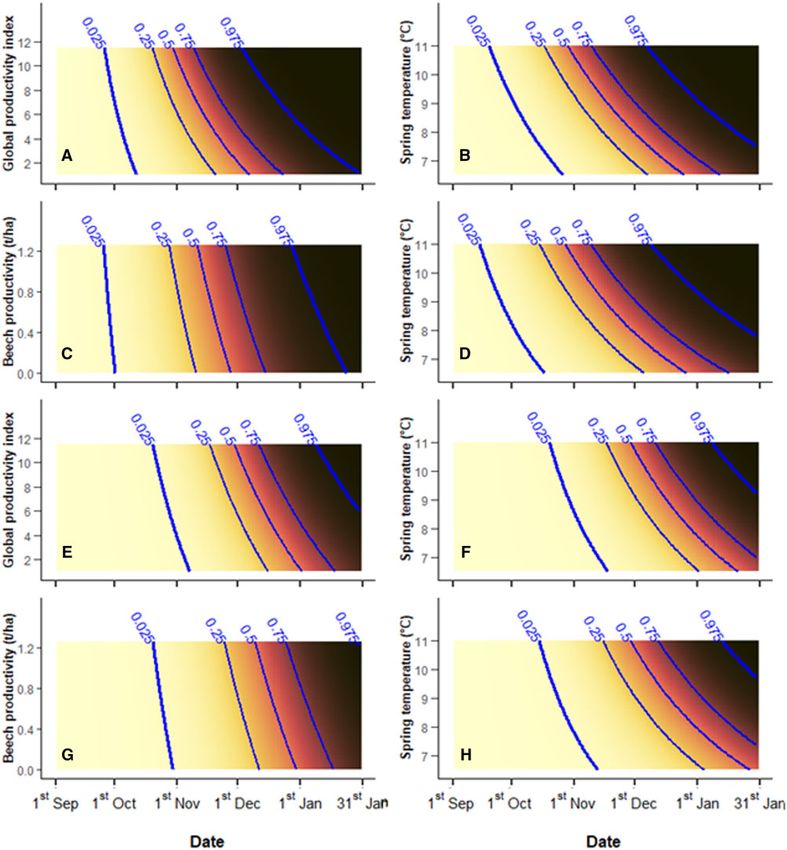
Interannual ovulation and pregnancy patterns predicted by 1S-ov, For adult female ovulation patterns, model 3A-ov included
1A-ov, 1S-pr, and 1A-pr are summarized in Figure 1. A marked spring average temperature, autumn rain, and chestnut productivity
interannual heterogeneity affected temporal patterns of both repro- as single variables and [beech productivity: date] and [spring tem-
ductive statuses considered, although the predicted portion of perature: date] as interaction terms (Supplementary Table S2b).
females achieving ovulation or pregnancy within the sampling Beech productivity only accounted for a slight shortening of the ovu-
period was always equal or close to 1 in both age classes. A number lation season (higher RS), with no effect on the timing of its onset
(Figure 2C). Conversely, warmer spring temperatures were associ-
of reproductive seasons were relatively early and short (hunting sea-
ated to both anticipated RT and higher RS of ovulation seasons
sons 2, 5, and 7), whereas others showed either a late onset (3, 6,
(Figure 2D).
and 10) or a longer duration (1 and 9). Likewise, the temporal dis-
The model 3S-pr, which explained subadult female pregnancy
tance between ovulation and pregnancy curves varied among the
patterns, included individual body mass and chestnut productivity
years, with the minimum value observed in hunting season 2 and the
as single variables in addition to the same interaction terms selected
maximum in 5 and 8. Finally, subadult and adult females showed
for ovulation patterns of the same age class, that is, [global product-
completely overlapped reproductive patterns in a number of hunting
ivity index: date] and [spring temperature: date]. When seed prod-
seasons (2, 6, and 7) and markedly divergent in other ones (3 and 4).
uctivity was higher, subadult female pregnancy showed an
On average, the date when the proportion of ovulated females
anticipated RT and a higher RS (Figure 2E). A similar pattern was
reached 0.5 corresponded to 82.46 (21 November) 6 14.67
observed for average spring temperature, though with a stronger ef-
(mean 6 SD) and 83.77 (23 November) 6 13.60 days from
fect in anticipating pregnancy RT (Figure 2F).
1 September in subadults and adults, respectively, without a statis-
The model 3A-pr, which accounted for adult female pregnancy
tically significant difference between the 2 age classes (t ¼ 0.55,
patterns, included individual body mass and chestnut productivity
P-value ¼ 0.60). A similar result was detected for pregnancy, as
as single predictor variables in addition to the same interaction
subadult females reached the middle point at 109.60 (19
terms selected for ovulation patterns of the same age class, that is,
December) 6 14.82 days from 1 September and adult females at
[beech productivity: date] and [spring temperature: date]. Their
115.61 (25 December) 6 17.88 days from 1 September, with the
effects on RT and RS were similar to those shown on adult female
paired t-test returning a non-significant difference (t ¼ 1.70,
ovulation, though isolines showed an overall delay (Figures 2G,H).
P ¼ 0.12). Conversely, the duration of the ovulation season (a
measure of RS) was shorter in subadult (96.54 6 9.46 days) than in
adult females (114.00 6 10.85 days) and this difference was statistical- Discussion
ly significant (t ¼ 3.84, P ¼ 0.0012). As 95% of subadult females
We showed that, in an ungulate species inhabiting temperate lati-
got pregnant in 94.20 6 10.65 days, whereas adult females in
tudes, breeding seasons can change in timing and duration, depend-
121.13 6 16.01 days from the onset, pregnancy season duration was
ing on environmental conditions. Both population RT and RS
significantly shorter in subadult females (t ¼ 4.43, P ¼ 0.0004).
widely varied among different years and our analytical approach
enabled to properly evaluate their dependence on the environment.
Step 2: factors influencing individual reproductive These phenomena were essentially due to the individual tendency to
status reproduce even when a harsh environment made the investment
Predictor variable sets included in the best model for the 4 GLMs risky in terms of offspring survival. Such population-level features
explaining the individual likelihood of ovulating and getting preg- likely entail a high resilience of the population reproductive patterns
nant are summarized in Table 1, whereas those selected for random against ecological perturbations and environmental changes as con-
forest analysis and dredge are summarized in Supplementary Table firmed by the extremely high average likelihood of females ovulating
S1. Standardized date and average spring temperature were included or getting pregnant by the end of the reproductive season in every
in all 4 best GLMs and positively affected both ovulation and preg- sampling year.
nancy rates in both age classes. Individual body mass only increased We observed a high temporal heterogeneity among yearly repro-
the likelihood of subadult females ovulating, whereas its positive ef- ductive patterns (Figure 1). However, in accordance with Servanty
fect on pregnancy ratio concerned both age classes. As for food et al. (2009), the model described in Step 1 predicted an average in-
availability, at least 1 predictor reflecting seed productivity was dividual likelihood of ovulating which reached values close to 1 be-
included in each best GLM. The relative abundance of adult males fore 31 January every year and in both age classes considered.
was not selected for any best GLM. Pregnancy followed similar patterns, thus proving that ovulationBrogi et al. Population-level plasticity of wild boar reproductive timing and synchrony 5
Downloaded from https://academic.oup.com/cz/advance-article/doi/10.1093/cz/zoab077/6371954 by guest on 06 November 2021
Figure 1. Ovulation (continuous lines) and pregnancy (dashed lines) patterns of subadult (red) and adult (blue) females throughout 10 hunting seasons in
Northern Apennines, Italy. Values were predicted by 4 GLMs with the interaction between date and hunting season as the only predictor variable (see the text for
more details). Color-shaded areas represent 95% confidence intervals.
rates represent a good wild boar pregnancy proxy. Interannual preg- boar populations (relying on artificial food, Macchi et al. 2010;
nancy delay variability in respect to ovulation was likely the effect Malmsten et al. 2017b; Bergqvist et al. 2018), our results showed
of a variable proportion of ovulated females failing to get pregnant. that, for adult and subadult females, an actual breeding season
However, thanks to their ability to repeat the estrus (Henry 1968; existed and was included within our sampling period. The minimal
Barrett 1978; Macchi et al. 2010), all female wild boar (subadult number of reproductive juvenile females detected in our study (823
and adult) were predicted to achieve pregnancy even in the years culled juvenile females, 30 ovulated, and 3 pregnant) may be a sign
with the highest delays (e.g., hunting seasons 5 and 8). Although of their contribution to reproduction being negligible or the conse-
minor reproductive events may occur all year round in other wild quence of the 5 months sampling period duration being insufficient6 Current Zoology, 2021, Vol. 0, No. 0
Table 1. Sets of explanatory variables included in the best GLM on the individual likelihood of: subadult females ovulating (2S-ov); adult
females ovulating (2A-ov); subadult females getting pregnant (2S-pr); and adult females getting pregnant (2A-pr).
Model Sub-dataset Reproductive state Best model formula
2S-ov Subadult females Ovulation Ovulated standardized date þ body mass þ spring temperature þ
autumn rain þ global productivity index
2A-ov Adult females Ovulation Ovulated standardized date þ spring temperature þ summer rain þ
autumn rain þ chestnut productivity þ beech productivity
2S-pr Subadult females Pregnancy Pregnant standardized date þ body mass þ spring temperature þ
summer rain þ chestnut productivity þ global productivity index
2A-pr Adult females Pregnancy Pregnant standardized date þ body mass þ spring temperature þ
Downloaded from https://academic.oup.com/cz/advance-article/doi/10.1093/cz/zoab077/6371954 by guest on 06 November 2021
chestnut productivity þ beech productivity
Standardized culling date, culling date expressed as days from 1 September; body mass, individual body mass (kg); season x temperature, average environmental
temperature recorded during the season x; season x rain, average daily rain precipitation recorded during the season x; productivity of species y, mast productivity
of the tree species y during the current year expressed as t/ha; global productivity index, index summarizing all tree species productivity during the current year
(see the text for more details).
to detect juvenile reproduction, which has been shown to occasion- Zerbe et al. 2012) and equatorial, seasonal breeding ungulates
ally occur in other wild boar populations ( Sprem et al. 2016; (whose reproductive phenology mainly relies on environmental
Gamelon et al. 2017). Collecting data all year round (possible in cues, Ogutu et al. 2015).
cases of wild boar hunting being performed during the whole year) The approach adopted to build Step 3 models enabled to evalu-
would be necessary to properly evaluate the reproductive contribu- ate ovulation and pregnancy temporal patterns of the population in
tion of different classes of females outside the core reproductive respect to the environment, that is, to monitor the breeding season
period, but it is worth noting that this was not the objective of this temporal onset, progress, and duration at varying environmental
study. conditions. Ovulation and pregnancy RTs were substantially antici-
Subadult females were significantly more synchronous than pated under good environmental conditions (i.e., higher resources
adults, likely on account of an overall higher homogeneity of their availability and warmer spring temperatures) in both age classes
individual conditions. Differently from the older class, all subadult (Figure 2), thus showing the high degree of ecological plasticity of
females belonged to the same cohort and most of them were at their wild boar reproductive phenology. The physiological phenomenon
first reproductive attempt (as confirmed by the almost null repro- was likely mediated by individual nutritional conditions (McGinnes
ductive rate observed in juvenile females) and had not to cope with and Downing 1977; Hamilton and Blaxter 1980; Flydal and
previous parental reproductive costs. Conversely, adult females had Reimers 2002; Wolcott et al. 2015), which were directly improved
different ages and might have coped with different costs related to either by resource abundance or by the advanced vegetation growth
their previous reproduction (Hamel et al. 2010). due to high spring temperatures.
The fact that the average likelihood of ovulating and getting The possibility to either plastically anticipate or delay breeding
pregnant reached values close to 1 within our sampling period seasons maximizes population reproductive outcomes under optimal
enabled an unambiguous interpretation of the Steps 2 and 3 analy- conditions, whereas increasing its resilience against ecological per-
ses: the effects of the environmental factors identified only either turbations. During favorable years, anticipated breeding seasons
anticipated or delayed changes of the reproductive status, without produce earlier births, which are known to increase offspring sur-
truly affecting the individual likelihood of ovulating and getting vival in ungulates (Côté and Festa-Bianchet 2001). In the case of
pregnant by the end of the reproductive season. This evidence helps wild boar, earlier births may directly reduce the young mortality
to understand environmental influence on female wild boar repro- caused by red fox (Vulpes vulpes) predation (Bassi et al. 2012) by
ductive status, which so far was widely investigated by focusing on producing a beneficial mismatch between the time when piglets are
the overall proportion of reproductive females (Fonseca et al. 2011; of vulnerable size and the time when fox food requirement is most
Bergqvist et al. 2018; Touzot et al. 2020) and seldom considering intense (young raising, from May onwards in Southern Europe,
the temporal dimension (Servanty et al. 2009). In this context, a Cavallini and Santini 1995). The potential to plastically anticipate
yearly proportion of reproductive females estimated without taking breeding seasons may result extremely beneficial also when facing
into account culling dates is prone to be substantially underesti- global change by softening or even preventing mismatches between
mated. In fact, females culled early in the hunting season with no births and the most favorable nutritional conditions for offspring. In
sign of ongoing ovulation or pregnancy and considered “not this respect, wild boar may represent an exceptional case of a species
reproductive” (Fonseca et al. 2011; Bergqvist et al. 2018; Touzot “pre-adapted” to global change, as already suggested (Vetter et al.
et al. 2020) should rather be considered “not reproductive yet.” 2015; Touzot et al. 2020). Conversely, when less resources are avail-
The influence of the standardized date was included in all the able, a delayed breeding season gives individuals more time to get
best models selected in Steps 2 and 3 (as single predictor and in the nutritional condition needed to reproduce. In so doing, a higher
interaction with environmental variables, respectively). Thus, it is proportion of mature individuals can achieve reproduction at the
suggested that photoperiodism still constrained wild boar RT, cost of an increased offspring mortality. The high hunting pressure
though its influence was not so strong if compared with that exerted may have increased the advantage of such a risky investment, as
over most ungulates inhabiting temperate regions. This evidence pla- individuals counting on a short life expectancy have to exploit every
ces wild boar at an intermediate position along an ideal continuum reproductive opportunity to maximize their fitness (Festa-Bianchet
between temperate ungulates (which rigidly rely on photoperiodism 2003). We observed no relationship between the number of culled
to time their reproduction, with minor environmental influence, adult males per female and ovulation and pregnancy temporalBrogi et al. Population-level plasticity of wild boar reproductive timing and synchrony 7
Downloaded from https://academic.oup.com/cz/advance-article/doi/10.1093/cz/zoab077/6371954 by guest on 06 November 2021
Figure 2. Predicted effect of the interaction between environmental variables and the standardized date on the proportion of: ovulating subadult females (A and
B), ovulating adult females (C and D), pregnant subadult females (E and F), and pregnant adult females (G and H), expressed by the chromatic scale (white ¼ low;
black ¼ high). Blue lines represent 0.025 (ovulation and pregnancy season onset), 0.25, 0.5, 0.75, and 0.975 (ovulation and pregnancy season end) isolines. Spring
temperature: average air temperature of previous spring ( C); Global productivity index: mast tree global productivity index (see the text for more details); Beech
productivity: beechnut productivity (t/ha).
patterns. This result is surprising in a heavily hunted population flexible reproductive involvement of subadult male wild boar. As we
(i.e., subject to adult male scarcity, Fernandez-Llario and Mateos- did not consider other population traits, such as density and struc-
Quesada 2003; Toı̈go et al. 2008) and appears in contrast with the ture, further investigations are needed to evaluate their potential ef-
results obtained for other ungulate species (Milner et al. 2007). fect on wild boar temporal reproductive patterns.
Nonetheless, it is consistent with the findings proposed by A number of environmental factors in interaction with the stand-
Diefenbach et al. (2019) on white tailed deer (Odocoileus virginia- ardized date were included as predictors in Step 3 best models, thus
nus) as well as with Brogi et al.’s (2021) hypothesis regarding the showing that good environmental conditions (higher spring8 Current Zoology, 2021, Vol. 0, No. 0
temperatures, higher food availability) enhanced RS and ultimately trigger its reproduction. This feature likely represents a key factor
led to shorter breeding seasons (Figure 2). We thus showed that, as for wild boar renowned ecological plasticity and ultimately con-
previously reported only for equatorial ungulates (Ogutu et al. tributes to its high success and worldwide spread (Massei et al.
2010, 2014), photoperiodic species inhabiting temperate regions 2015; Markov et al. 2019).
also have the potential to adjust breeding season length depending
on environmental conditions. In the monitored population, RS was
enhanced by higher spring temperatures in both age classes and by Acknowledgments
global seed and beechnut productivity in subadult and adult females, We are grateful to all hunters, researchers, students, and volunteers who con-
respectively. Breeding seasons following hot springs were 40% tributed to data collection, especially E. Bertolotto, N. Cappai, E. Donaggio,
shorter in respect to those following cold springs in both age classes. and D. Battocchio. We also wish to thank C. Pole for kindly editing the
Downloaded from https://academic.oup.com/cz/advance-article/doi/10.1093/cz/zoab077/6371954 by guest on 06 November 2021
Global seed productivity had a similar impact (shortening of 36%) English version of this manuscript. The Regional Hydrological Service of
Tuscany provided meteorological data. The Provincial Administration of
on subadult female ovulation seasons, whereas years with a high
Arezzo and the Italian Ministry of Education, University and Research (PRIN
beechnut productivity reduced adult female ovulation season length
2010-2011, 20108 TZKHC) financially and logistically supported the re-
of 20% in respect to less productive ones. These environmental
search. S.G .was supported by the FAR 2020 of the University of Sassari.
factors likely induced a plastic anticipation of individual reproduct-
ive phenology but heterogeneously affected each individual.
Conversely, only the average population RT would have been modi- Authors’ Contributions
fied, with no effect on inter-individual differences and, therefore, on
E.M., S.G., R.B., and M.A. originally formulated the idea. R.C. and E.B. con-
RS (as in the case of other environmental factors included as single ducted fieldwork. R.B., E.M., and S.G. collaborated in imaging and perform-
predictors in Step 3 best models). We can suppose that, when the ing analysis. R.B. wrote the original draft of the manuscript. S.G., E.M.,
main food resources were more abundant, all females reached the M.A., and R.C. provided editorial advice. M.A. provided materials tools and
threshold nutritional condition needed to reproduce early and contributed to funding acquisition.
achieved ovulation as soon as their internal photoperiodism enabled
them to. This optimal nutritional condition induced a quite homo-
genous distribution of ovulation within the population. Conversely, Supplementary Material
in case of low resource availability, the pre-existing variability of in- “Supplementary material can be found at https://academic.oup.com/cz.”
dividual conditions would be unaltered or even enhanced. For in-
stance, foraging strategies would be more diversified, with a number
of individuals either being able to outcompete the others for the References
scarce resources available or better exploiting secondary food items. Barrett R, 1978. The feral hog at Dye Creek ranch, California. Hilgardia 46:
The whole breeding season RT would be delayed (as observed, for 322–325.
example, when the global productivity index was low), though a Bassi E, Donaggio E, Marcon A, Scandura M, Apollonio M, 2012. Trophic
number of individuals would be less affected than others by resource niche overlap and wild ungulate consumption by red fox and wolf in a
mountain area in Italy. Mammal Biol- Zeitschr Säugetier 77:369–376.
scarceness and still be able to pursue an early reproduction, thus
Bergqvist G, Paulson S, Elmhagen B, 2018. Effects of female body mass and
inducing a substantial RS reduction. In this context, spring tempera-
climate on reproduction in northern wild boar. Wildlife Biol 2018: 1.
tures may have acted as a proxy of the vegetation growth season
Bisi F, Chirichella R, Chianucci F, Von Hardenberg J, Cutini A et al., 2018.
and regulated abundance and temporal occurrence of food resources Climate, tree masting and spatial behaviour in wild boar (Sus scrofa L.): in-
other than mast seeds. sight from a long-term study. Ann For Sci 75:46.
The possibility to regulate RS in respect to the environmental Bradshaw WE, Holzapfel CM, 2007. Evolution of animal photoperiodism.
conditions may provide several advantages to the population repro- Ann Rev Ecol Evol Syst 38:1–25.
ductive outcomes. In particular, birthdates may be highly concen- Breiman L, 2001. Random forests. Mach Learn 45:5–32.
trated when, during the mating season, environmental conditions Briedermann L, 1990. Wild boars 1–540.
are good (and likely induced a high nutritional condition of Brogi R, Chirichella R, Brivio F, Merli E, Bottero E et al., 2021.
Capital-income breeding in wild boar: a comparison between two sexes. Sci
females). When favored by resource availability, the advantageous
Rep 11:4579.
(Côté and Festa-Bianchet 2001) phenotypic trait of early reproduc-
Canu A, Scandura M, Merli E, Chirichella R, Bottero E et al., 2015.
tion may thus be evenly distributed within the population. We can
Reproductive phenology and conception synchrony in a natural wild boar
hypothesize that a higher birth synchrony may also reduce predation population. Hystrix 26(2):77–84.
risk by saturating the number of newborns that predators (wolves, Cavallini P, Santini S, 1995. Timing of reproduction in the red fox Vulpes
Canis lupus, and foxes in the monitored study area, Bassi et al. vulpes. Zeitschr Saugetier 60:337–342.
2012) can catch per time unit (dilution effect, Darling 1938). Chianucci F, Ferrara C, Bertini G, Fabbio G, Tattoni C et al., 2019.
Conversely, under suboptimal environmental conditions, the Multi-temporal dataset of stand and canopy structural data in temperate
enhanced phenotypic diversity showed by the population reproduct- and Mediterranean coppice forests. Ann For Sci 76:80.
ive phenology may produce more scattered birthdates. This may re- Côté SD, Festa-Bianchet M, 2001. Birthdate, mass and survival in mountain
sult in a more efficient resource partitioning among individuals that goat kids: effects of maternal characteristics and forage quality. Oecologia
127:230–238.
are raising young (Ims 1990). However, more scattered birthdates
Darling FF, 1938. Bird flocks and the breeding cycle; a contribution to the
amount to a population trait and therefore may not be shaped dir-
study of avian sociality. Cambridge University Press.
ectly by evolution and, as explained above, rather seems the conse- Diefenbach DR, Alt GL, Wallingford BD, Rosenberry CS, Long ES, 2019.
quence of the combination of individual adaptive features. Effect of male age structure on reproduction in white-tailed deer. J Wildlife
We provided the first evidence of breeding season length ad- Manage 83:1368–1376.
justment depending on environmental conditions in a species English AK, Chauvenet ALM, Safi K, Pettorelli N, 2012. Reassessing the deter-
living in temperate regions and relying on photoperiodism to minants of breeding synchrony in ungulates. PLoS ONE 7:e41444.Brogi et al. Population-level plasticity of wild boar reproductive timing and synchrony 9
Fernández GJ, Carro ME, Llambı́as PE, 2020. Spatial and temporal variation Merli E, Grignolio S, Marcon A, Apollonio M, 2017. Wild boar under fire: the
in breeding parameters of two south-temperate populations of house wrens. effect of spatial behaviour, habitat use and social class on hunting mortality.
J Field Ornithol 91:13–30. J Zool 303:155–164.
Fernandez-Llario P, Mateos-Quesada P, 2003. Population structure of the Milner JM, Nilsen EB, Andreassen HP, 2007. Demographic side effects of se-
wild boar Sus scrofa in two Mediterranean habitats in the western Iberian lective hunting in ungulates and carnivores. Conservat Biol 21:36–47.
Peninsula. Folia Zool PRAHA 52:143–148. Nussbaumer A, Waldner P, Apuhtin V, Aytar F, Benham S et al., 2018. Impact
Festa-Bianchet M, 2003. Exploitative wildlife management as a selective pres- of weather cues and resource dynamics on mast occurrence in the main for-
sure for the life-history evolution of large mammals. Anim Behav Wildlife est tree species in Europe. For Ecol Manage 429:336–350.
Conserv 1:191–207. Ogutu JO, Owen-Smith N, Piepho HP, Dublin HT, 2015. How rainfall vari-
Findlay CS, Cooke F, 1982. Breeding Synchrony in the lesser snow goose ation influences reproductive patterns of African Savanna ungulates in an
Anser caerulescens caerulescens. I. Genetic and environmental components equatorial region where photoperiod variation is absent. PLoS ONE 10:
Downloaded from https://academic.oup.com/cz/advance-article/doi/10.1093/cz/zoab077/6371954 by guest on 06 November 2021
of hatch date variability and their effects on hatch synchrony. Evolution 36: e0133744.
342. Ogutu JO, Piepho HP, Dublin HT, 2014. Responses of phenology, synchrony
Flydal K, Reimers E, 2002. Relationship between calving time and physical and fecundity of breeding by African ungulates to interannual variation in
condition in three wild reindeer Rangifer tarandus populations in southern rainfall. Wildlife Res 40:698.
Norway. Wildlife Biol 8:145–151. Ogutu JO, Piepho HP, Dublin HT, Bhola N, Reid RS, 2010. Rainfall extremes
Fonseca C, da Silva AA, Alves J, Vingada J, Soares AMVM, 2011. explain interannual shifts in timing and synchrony of calving in topi and
Reproductive performance of wild boar females in Portugal. Eur J Wildlife warthog. Popul Ecol 52:89–102.
Res 57:363–371. Post E, Pedersen C, Wilmers CC, Forchhammer MC, 2008. Warming, plant
Gamelon M, Focardi S, Baubet E, Brandt S, Franzetti B et al. 2017. phenology and the spatial dimension of trophic mismatch for large herbi-
vores. Proc Royal Soc B Biol Sci 275:2005–2013.
Reproductive allocation in pulsed-resource environments: a comparative
R Development Core Team, 2015. R: A Language and Environment for
study in two populations of wild boar. Oecologia 183:1065–1076.
Statistical Computing. Vienna, Austria: R Foundation for Statistical
Garel M, Solberg EJ, Sæther B, Grøtan V, Tufto J et al., 2009. Age, size, and
Computing.
spatiotemporal variation in ovulation patterns of a seasonal breeder, the
Ruf T, Fietz J, Schlund W, Bieber C, 2006. High survival in poor years: life his-
Norwegian moose Alces alces. Am Nat 173:89–104.
tory tactics adapted to mast seeding in the edible dormhouse. Ecology 87:
Hamel S, Côté SD, Festa-Bianchet M, 2010. Maternal characteristics and en-
372–381.
vironment affect the costs of reproduction in female mountain goats.
Santos P, Fernández-Llario P, Fonseca C, Monzón A, Bento P et al., 2006.
Ecology 91:2034–2043.
Habitat and reproductive phenology of wild boar Sus scrofa in the western
Hamilton WJ, Blaxter KL, 1980. Reproduction in farmed red deer. J Agric Sci
Iberian Peninsula. Eur J Wildlife Res 52:207–212.
95:261–273.
Servanty S, Gaillard J, Toı̈go C, Brandt S, Baubet E, 2009. Pulsed resources
Henry VG, 1968. Length of estrous cycle and gestation in European wild hogs.
and climate-induced variation in the reproductive traits of wild boar under
J Wildlife Manage 32:406.
high hunting pressure. J Anim Ecol 78:1278–1290.
Hertel AG, Royauté R, Zedrosser A, Mueller T, 2020. Biologging reveals indi-
Sinclair ARE, Mduma SA, Arcese P, 2000. What determines phenology and
vidual variation in behavioral predictability in the wild. J Anim Ecol 90:
synchrony of ungulate breeding in Serengeti? Ecology 81:2100–2111.
723–737.
Sprem N, Piria M, Prd-un S, Novosel H, Treer T, 2016. Variation of wild boar
Ims RA, 1990. The ecology and evolution of reproductive synchrony. Trend
reproductive performance in different habitat types: implications for man-
Ecol Evol 5:135–140.
agement. Russian J Ecol 47:96–103.
Macchi E, Cucuzza AS, Badino P, Odore R, Re F et al., 2010. Seasonality of re-
Symonds MR, Moussalli A, 2011. A brief guide to model selection, multimo-
production in wild boar Sus scrofa assessed by fecal and plasmatic steroids. del inference and model averaging in behavioural ecology using Akaike’s in-
Theriogenology 73:1230–1237. formation criterion. Behav Ecol Sociobiol 65:13–21.
Malmsten A, Jansson G, Dalin AM, 2017a. Post-mortem examination of the Toı̈go C, Servanty S, Gaillard JM, Brandt S, Baubet E, 2008. Disentangling
reproductive organs of female wild boars Sus scrofa in Sweden. Reprod natural from hunting mortality in an intensively hunted wild boar popula-
Domestic Anim 52:570–578. tion. J Wildlife Manage 72:1532–1539.
Malmsten A, Jansson G, Lundeheim N, Dalin A-M, 2017b. The reproductive Touzot L, Schermer É, Venner S, Delzon S, Rousset C et al., 2020. How does
pattern and potential of free ranging female wild boars Sus scrofa in increasing mast seeding frequency affect population dynamics of seed con-
Sweden. Acta Vet Scand 59:52. sumers? Wild boar as a case study. Ecol Appl 30:e02134.
Markov N, Pankova N, Morelle K, 2019. Where winter rules: modeling wild Vetter SG, Ruf T, Bieber C, Arnold W, 2015. What is a mild winter? Regional
boar distribution in its north-eastern range. Sci Total Environ 687: differences in within-species responses to climate change. PLoS ONE 10:
1055–1064. e0132178.
Mason THE, Chirichella R, Richards SA, Stephens PA, Willis SG et al., 2011. Wolcott DM, Reitz RL, Weckerly FW, 2015. Biological and environmental
Contrasting life histories in neighbouring populations of a large mammal. influences on parturition date and birth mass of a seasonal breeder. PLoS
PLoS ONE 6:e28002. ONE 10:e0124431.
Massei G, Kindberg J, Licoppe A, Gacic D, Sprem N et al., 2015. Wild boar Zerbe P, Clauss M, Codron D, Bingaman Lackey L et al., 2012. Reproductive
populations up, numbers of hunters down? A review of trends and implica- seasonality in captive wild ruminants: implications for biogeographical
tions for Europe: wild boar and hunter trends in Europe. Pest Manage Sci adaptation, photoperiodic control, and life history. Biol Rev 87:965–990.
71:492–500. Zuur A, Ieno EN, Walker N, Saveliev AA, Smith GM, 2009. Mixed effects
McGinnes BS, Downing RL, 1977. Factors affecting the peak of white-tailed models and extensions in ecology with R. Berlin, Germany: Springer Science
deer fawning in Virginia. J Wildlife Manage 41:715–719. & Business Media.You can also read