IUCRJ WHOLE PAIR DISTRIBUTION FUNCTION MODELING: THE BRIDGING OF BRAGG AND DEBYE SCATTERING THEORIES - MSS

Page created by Allan Sandoval
 
CONTINUE READING
IUCRJ WHOLE PAIR DISTRIBUTION FUNCTION MODELING: THE BRIDGING OF BRAGG AND DEBYE SCATTERING THEORIES - MSS
IUCrJ (2021). 8, doi:10.1107/S2052252521000324   Supporting information

IUCrJ
Volume 8 (2021)

Supporting information for article:

Whole Pair Distribution Function Modeling: the Bridging of Bragg
and Debye Scattering Theories

Alberto Leonardi
IUCRJ WHOLE PAIR DISTRIBUTION FUNCTION MODELING: THE BRIDGING OF BRAGG AND DEBYE SCATTERING THEORIES - MSS
research papers

                                                     Whole pair distribution function modeling: the
IUCrJ
ISSN 2052-2525
                                                     bridging of Bragg and Debye scattering theories

MATERIALS | COMPUTATION
                                                     Alberto Leonardi*

                                                     Institute for Multiscale Simulation, IZNF, Friedrich-Alexander-Universität Erlangen-Nürnberg Cauerstrasse, 3, Erlangen,
                                                     Bavaria 91052, Germany. *Correspondence e-mail: alberto.leonardi@fau.de

                                                     Supporting information

                                                     S1. Crystal shape and size dispersions
Keywords: powder scattering; pair distribution
functions; Debye Scattering equation; line profile   The dispersion of the crystal shapes and sizes is captured via combination of the
analysis; whole-powder-pattern modeling; Bragg       contributions from the different sample fractions. For any given crystal with shape
peaks; computing efficiency; common-volume
                                                       , the common volume function (CVF), ( , ), is normalized with the shape
functions.
                                                     volume ∀ , such that ( = 0, ) = 1, where is the pair-distance, and is the
                                                     size of the crystal. Therefore, besides to account for the probability of observing a
                                                     crystal with a given shape and size, ( ), the contributions to the pair distribution
                                                     function are weighted with the reciprocal of the crystal volumes as,
                                                                            ∑ ∑             ( , )               ( )
                                                               V( ) =           ∑ ∑                       ( )
                                                                                                                       ,                                                   (S1)

                                                     where     = ∀ ⁄ is a constant dependent on the crystal shape.
                                                     The size-distribution can be convoluted with the CVF for any given shape as,
                                                                            ∑       ∫           ( , )           ( )
                                                               V( ) =                                                      ,                                               (S2)
                                                                                ∑           ∫             ( )

                                                     where ( ) is the probability distribution function (Figure S2). To facilitate the
                                                     solution of the integrals, the CVF can be approximated with a polynomial function
                                                     with coefficients , as,

                                                                                    ∑            ,               , if      ≤
                                                               V ( , )=                                                            .                                       (S3)
                                                                                        0                       , if       ≥

                                                     Given piecewise polynomial functions with two intervals are better suited to
                                                     approximate the CVF of concave and non-regular shape, Eq. S3 becomes

                                                                        ⎧∑                           ,            , if         ≤
                                                                        ⎪
                                                                V ( , )= ∑                           ,            , if         ≥       ≥ ,                                 (S4)
                                                                        ⎨
                                                                        ⎪0                                       , if          ≥
                                                                        ⎩
                                                     where      , and  , are the polynomial coefficients for the two consecutive
                                                     intervals, and and are characteristic shape constants.

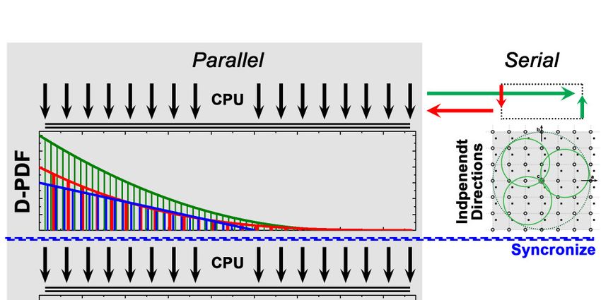
                                                     S2. Algorithm parallelization
                                                     The modeling of both the intensity profile and the pair distribution function (PDF)
                                                     is performed through three subsequent computing stages (Figure S4).

                                                     S2.1. Estimation of the directional-pair distribution function (D-PDF)
                                                     In this stage, synchronous and asynchronous operations are performed by different
                                                     CPU threads. Child processes synchronize to retrieve the directional parameters
                                                     from the master process, which computes the independent directions using a serial
IUCrJ (2021). 8                                                                                          https://doi.org/10.1107/S2052252521000324                   1 of 5
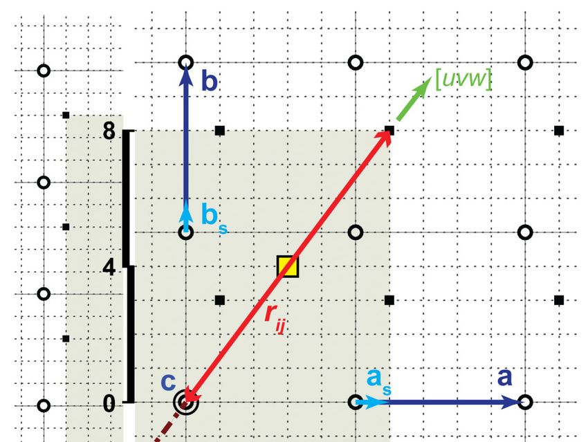
IUCRJ WHOLE PAIR DISTRIBUTION FUNCTION MODELING: THE BRIDGING OF BRAGG AND DEBYE SCATTERING THEORIES - MSS
research papers
algorithm. The child threads compute the D-PDFs without any                             Asynchronous computing processes perform this task for a
synchronization, inherently balancing their workload. A pair of                         different set of pair-distances (i.e., non-empty memory
per-thread memory arrays are updated with the estimated                                 locations).
probability counts and the difference between actual and
recorded pair-distances.                                                                S2.3. Modeling of the scattering profiles
                                                                                        Experimental-like scattering profiles are computed: the
S2.2. Solution of the whole pair distribution function
                                                                                        intensity profile via Debye scattering equation (DSE), and the
(WPDF)
                                                                                        PDF resampling the high accuracy whole PDF. Both the
The data collected by each thread in the first stage are collected.                     scattering profiles are corrected to match the corresponding
The estimated probabilities and pair distance differences are                           experimental representation (e.g., removal of the small-angle
summed. The recorded pair distances are, then, corrected.                               contribution to the PDF, and rescaling with the pair-distance).

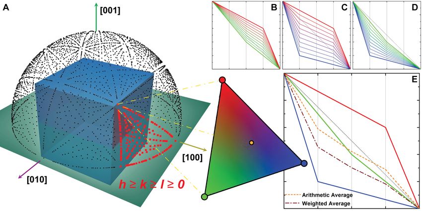
Figure S1 Interpolation of tabulated common volume functions. A, projection on a unit-sphere of the directions for which are recorded the CVFs. In case the
correlation between a site and its own repetition is considered, the complete set (black dots) is inferred from a subset in the first octant (red dots). A triangular sector
from the sphere surface is mapped with an RGB color scheme using the barycentric coordinates as the R, G, and B factors. B, C, and D, variation of the CVF
interpolated along the edges of the triangular sector. E, Interpolation of the two-intervals piecewise CVFs tabulated for the directions associated with the triangular
sector corners. In B to E, the intervals into which the CVFs are divided are marked (gray line). Note that the CVFs for the sector corners are only example profiles,
and they were not computed from any shape.

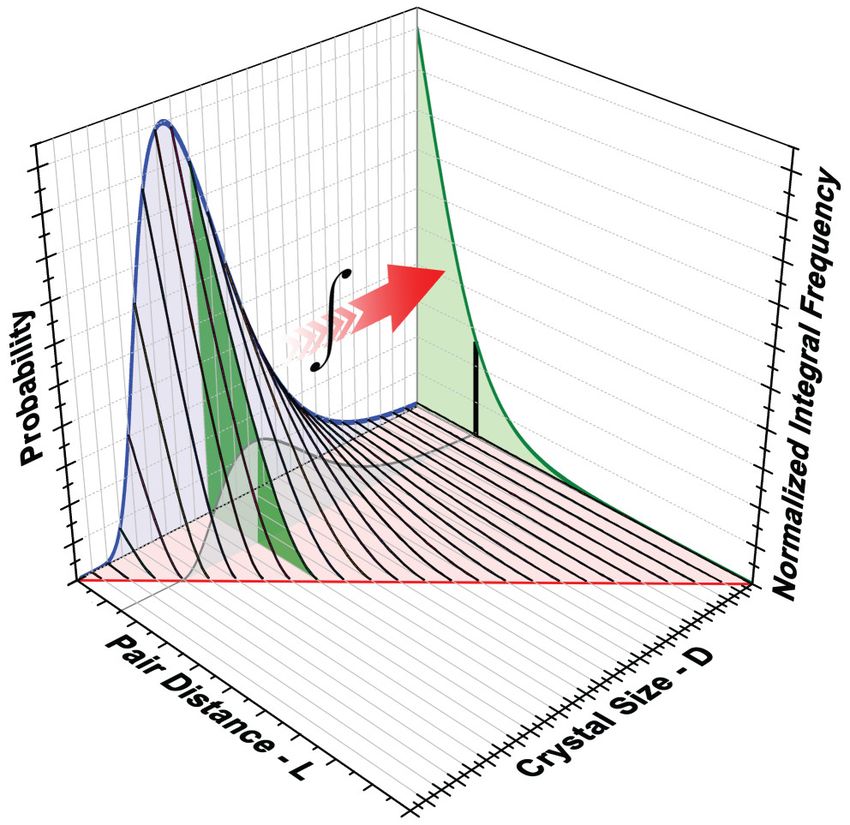
                                                                                        Figure S2 Graphical representation of the convolution of the CVF with
                                                                                        the size dispersion. The CVF profile (black line) scale with the crystal size (red
                                                                                        line) and the size probability distribution function (blue line). The integral
                                                                                        frequency for the dispersion of crystals’ size (green line) is computed as the
                                                                                        area under the cross-section of the CVFs surface for constant pair distance (gray
                                                                                        line).

2 of 5        Alberto Leonardi • Whole pair distribution function modeling                                                                            IUCrJ (2021). 8
IUCRJ WHOLE PAIR DISTRIBUTION FUNCTION MODELING: THE BRIDGING OF BRAGG AND DEBYE SCATTERING THEORIES - MSS
research papers

Figure S3 Site periodicity in the service lattice system. Cubic crystalline            Figure S4 Algorithm parallelization. Computing stages used to model both
lattice system (continuous gray line) with occupied sites of relative coordinates      the intensity profile and the pair distribution function (PDF).
(0,0,0) and (1,3,0)/5 (black open circle and full square, respectively). Note
that the positive quadrant is magnified. All the occupied sites are at the nodes
of the service lattice (dotted gray line) of normalization factor = 5. The vector
pair distance aligned with the direction [          ] that binds the origin with the
(6,8,0)⁄5 site is shown to intersect also the site (3,4,0)⁄5 that belongs to the
service lattice system. The same site type repeat along the [uvw] direction at
constant step intervals with coprime triplet (3,4,0) the step interval in the
crystalline lattice system.

IUCrJ (2021). 8                                                                  Alberto Leonardi • Whole pair distribution function modeling        3 of 5
IUCRJ WHOLE PAIR DISTRIBUTION FUNCTION MODELING: THE BRIDGING OF BRAGG AND DEBYE SCATTERING THEORIES - MSS
research papers

Figure S5 Map of the library of shapes for which the CVF coefficients were tabulated. The CVF coefficients were computed for a set of polyhedral shapes
bounded by a single family of planes (hkl indices in the map) and for a set of truncated cubes with 200 degrees of truncation. The shapes were separated into
homogeneous groups (I to IX) according to the set of edges and corners angles. The shapes are colored according to the surface-to-volume ratio (color bar) assuming
the polyhedral crystals with volume 103 nm3. The CVF coefficients were calculated for 163 positively defined independent directions described by triplets of integers
with none index larger than 9 (2000 data point per direction). The values were interpolated either with a single cubic or a pair of cubic functions. The data were
formatted to be compatible with the software package PM2K. Because of size limitation, the complete data set is available on request.

4 of 5       Alberto Leonardi • Whole pair distribution function modeling                                                                       IUCrJ (2021) 8.
research papers

Table S1 Analytical expression of the common volume functions (CVF). Unless for the sphere shape, the CVF is a function of the observed direction ( , , )
positively defined in a Cartesian space such as ‖ , , ‖ = 1. Whereas for the cube, the tetrahedron, and the octahedron the direction components are reordered
such that ≥ ≥ ≥ 0, for the cylinder and hexagonal prism is aligned with the shape axes and is normal to a pair of opposite hexagonal sides. The cube
and octahedron shapes are assumed to be bounded by {1,0,0} and {1,1,1} planes, respectively. The tetrahedron is assumed to be bounded by the (1,1,1), (1, 1, 1),
(1, 1, 1), and (1, 1, 1) planes. Depending on the shape, is: the diameter of the sphere; the edge length of the cube, the tetrahedron, and the octahedron; the height
and the base diameter of the cylinder, or distance between a pair of opposite sides of the hexagonal prism. The equations are written for 0 ≤ ≤ ⁄ . The CVF
for the hexagonal prism split into two pieces at = ⁄ ∗ .

    Shape           Case                                                                Common Volume Function                                                                                 Boundary (K)
                                      3          1
    Sphere              -        1−          +                                                                                                                                                              1
                                      2          2

     Cube               -        1−( +        + )               +(      +               +       )             −

                    ≥       +    1 − 3√2             +6     2
                                                                        − 2√2               3                                                                                                           √2
 Tetrahedron
                                      3( +       + )                 3( +               + )2                                  3
                                                                                                                                                                                                        +       +
                    ≤       +    1−                             +                                            − 2√2
                                           √2                                       2                                                                                                                       √2
                                                                2       2                               3             2            2            3           3
                                      3              3( −           −       )                   −           +3 (          +            ) + 2(       +           )                                       +       +
                    ≥       +    1−            +                                            −
                                      √2                        2                                                         2√2                                                                               √2
  Octahedron
                                                                                2                                                                   3               3           3
                                      3( +       + )                 −3[            + ( − )2 − 2 ( + )]                                                 +               +           −3                  +       +
                    ≤       +    1−                             +                                                                               −
                                           2√2                                                      4                                                                       √2                              √2

                                                 2                      2               2                     2           2                             2               2
   Cylinder             -         1−                  cos                   +                       −             +                        1−(              +               )                 max       ,           +

                                                                                                                                                                                                                        ∗
                                                   2                                                                              4 1                                                                           1
                                  1−                 1−                         2 − √3 +                                  −           −                                                             ≤
                        ≤1                         3                                                                              3 2                                                                   √3 −
                          √3
                        ≥
                          2                      1                                                                                                                                                          √3 +
                                  1−               2 − √3 +                                     2 − √3 −                                                                                      max       ,
                                                 3                                                                                                                                                            2

                                                   2                                                                              4 1                                                                           1   ∗

 Hexagonal        ⎧ ≤ √3          1−                 1−                         2 − √3 +                                  −           −                                                                     ≤
                                                   3                                                                              3 2
   Prism               2
                  ⎨    1
                    ≥                            2                                                                                                                                                          √3 +
                  ⎩    2          1−               1−                       2 − √3 +                                                                                                          max       ,
                                                 3                                                                                                                                                            2
                                                                                                                                                                                                                        ∗
                                                   2                                                                              1                                                                             1
                          1       1−                 1−                         2 − √3 +                                  −         1 − √3 +                                                        ≤
                        ≤                          3                                                                              3                                                                     √3 +
                          2
                        ≥0                       2
                                  1−               1−                       2 − √3 +                                                                                                                max{ , }
                                                 3

IUCrJ (2021). 8                                                                                 Alberto Leonardi • Whole pair distribution function modeling                                                     5 of 5
You can also read