LEARNING FROM RULES GENERALIZING LABELED EXEMPLARS
←
→
Page content transcription
If your browser does not render page correctly, please read the page content below
Published as a conference paper at ICLR 2020

                                         L EARNING FROM RULES G ENERALIZING L ABELED
                                         E XEMPLARS
                                          Abhijeet Awasthi         Sabyasachi Ghosh     Rasna Goyal Sunita Sarawagi
                                          Department of Computer Science and Engineering
                                          Indian Instiute of Technology Bombay
                                          Mumbai, Maharashtra 400076, India
                                          {awasthi,sghosh,goyalrasna,sunita}@cse.iitb.ac.in
arXiv:2004.06025v2 [cs.LG] 15 May 2020

                                                                                       A BSTRACT
                                                  In many applications labeled data is not readily available, and needs to be col-
                                                  lected via pain-staking human supervision. We propose a rule-exemplar method
                                                  for collecting human supervision to combine the efficiency of rules with the qual-
                                                  ity of instance labels. The supervision is coupled such that it is both natural for
                                                  humans and synergistic for learning. We propose a training algorithm that jointly
                                                  denoises rules via latent coverage variables, and trains the model through a soft
                                                  implication loss over the coverage and label variables. The denoised rules and
                                                  trained model are used jointly for inference. Empirical evaluation on five different
                                                  tasks shows that (1) our algorithm is more accurate than several existing meth-
                                                  ods of learning from a mix of clean and noisy supervision, and (2) the coupled
                                                  rule-exemplar supervision is effective in denoising rules.

                                         1    I NTRODUCTION
                                         With the ever-increasing reach of machine learning, a common hurdle to new adoptions is the lack
                                         of labeled data and the pain-staking process involved in collecting human supervision. Over the
                                         years, several strategies have evolved. On the one hand are methods like active learning and crowd-
                                         consensus learning that seek to reduce the cost of supervision in the form of per-instance labels. On
                                         the other hand is the rich history of rule-based methods (Appelt et al., 1993; Cunningham, 2002)
                                         where humans code-up their supervision as labeling rules. There is growing interest in learning
                                         from such efficient, albiet noisy, supervision (Ratner et al., 2016; Pal & Balasubramanian, 2018;
                                         Bach et al., 2019; Sun et al., 2018; Kang et al., 2018). However, clean task-specific instance labels
                                         continue to be critical for reliable results (Goh et al., 2018; Bach et al., 2019) in spite of easy
                                         availability of pre-trained models (Sun et al., 2017; Devlin et al., 2018).
                                         In this paper we propose a unique blend of cheap coarse-grained supervision in the form of rules
                                         and expensive fine-grained supervision in the form of labeled instances. Instead of supervising rules
                                         and instance labels independently, we propose that each labeling rule be attached with exemplars of
                                         where the rule correctly ’fires’. Thus, the rule can be treated as a noisy generalization of those exem-
                                         plars. Often rules are coded up only after inspecting data. As a human inspects instances, he labels
                                         them, and then generalizes them to rules. Thus, humans provide paired supervision of rules and
                                         exemplars demonstrating correct deployment of that rule. We explain further with two illustrative
                                         applications. Our examples below are from the text domain because rules have been traditionally
                                         used in many NLP tasks, but our learning algorithm is agnostic to how rules are expressed.

                                         Sentiment Classification Consider an instance I highly recommend this modest
                                         priced cellular phone that a human inspects for a sentiment labeling task. After labeling
                                         it as positive, he can easily generalize it to a rule Contains ’highly recommend’ →
                                         positive label. This rule generalizes to several more instances, thereby eliminating the need
                                         of per-instance labeling on those. However, the label assigned by this rule on unseen instances may
                                         not be as reliable as the explicit label on this specific exemplar it generalized. For example, it misfires
                                         on I would highly recommend this phone if it weren’t for their poor
                                         service.
                                             Code and datasets available at https://github.com/awasthiabhijeet/Learning-From-Rules

                                                                                             1
Published as a conference paper at ICLR 2020
Slot-filling Consider a slot-filling task on restaurant reviews over labels like cuisine,
location, and time. When an annotator sees an instance like: what chinese
restaurants in this city have good reviews?, after labeling token chinese
as cuisine, he generalizes it to a rule: (.*ese|.*ian|mexican) restaurants →
(cuisine) restaurants. This rule matches hundreds of instances in the unlabeled set, but
could wrongly label a phrase like these restaurants. Our focus in this paper is developing
algorithms for training models under such coupled rule-exemplar supervision. Our main challenge
is that the labels induced by the rules are more noisy than instance-level supervised labels because
humans tend to over generalize (Tessler & Goodman, 2019) as we saw in the illustrations above.
Learning with noisy labels with or without additional clean data has been a problem of long-standing
interest in ML (Khetan et al., 2018; Zhang & Sabuncu, 2018; Ren et al., 2018b; Veit et al., 2017;
Shen & Sanghavi, 2019). However, we seek to design algorithms that better capture rule-specific
noise with the help of exemplars around which we have supervision that the rule fired correctly. We
associate a latent random variable on whether a rule correctly ’covers’ an instance, and jointly learn
the distribution among the label and all cover variables. This way we simultaneously train the clas-
sifier with corrected rule-label examples, and restrict over-generalized rules. The denoised rules are
used during inference to further boost accuracy of the trained model. In summary our contributions
in this paper are as follows:
Our contributions (1) We propose the paradigm of supervision in the form of rules generaliz-
ing labeled exemplars that is natural in several applications. (2) We design a training method that
simultaneously denoises over-generalized rules via latent coverage variables, and trains a classifi-
cation model with a soft implication loss that we introduce. (3) Through experiments on five tasks
spanning question classification, spam detection, sequence labeling, and record classification we
show that our proposed paradigm of supervision enables an effective synergy between rule-level
and instance-level supervision. (4) We compare our algorithm to several recent frameworks for
learning with noisy supervision and constraints, and show much better results with our method.
2 T RAINING WITH RULES AND E XEMPLARS
We first formally describe the problem of learning from rules generalizing examplars on a classi-
fication task. Let X denote the space of instances and Y = {1, . . . , K} denote the space of class
labels. Let the set of labeled examples be L = {(x1 , `1 , e1 ), . . . , (xn , `n , en )} where xi ∈ X is an
instance, `i ∈ Y is its user-provided label, and ei ∈ {R1 , . . . , Rm , ∅} denotes that xi is an exemplar
for rule ei . Some labeled instances may not be generalized to rules and for them ei = ∅. Also, a
rule can have more than one exemplar associated with it. Each rule Rj could be a blackbox function
Rj : x 7→ {`j , ∅} that takes as input an instance x ∈ X and assigns it either label `j or no-label.
When the ith labeled instance is an exemplar for rule Rj (that is, ei = Rj ), the label of the instance
`i should be `j . Additionally, we have a different set of unlabeled instances U = {xn+1 , . . . , xN }.
The cover set Hj of rule Rj is the set of all instances in U ∪ L for which Rj assigns a noisy label
`j . An instance may be covered by more than one rule or no rule at all, and the labels provided by
these rules may be conflicting. Our goal is to train a classification model Pθ (y|x) using L and U
to maximize accuracy on unseen test instances. A baseline solution is to use Rj to noisily label the
covered U instances using majority or other consensus method of resolving conflicts. We then train
Pθ (y|x) on the noisy labels using existing algorithms for learning from noisy and clean labels (Veit
et al., 2017; Ren et al., 2018b). However, we expect to be able to do better by learning the systematic
pattern of noise in rules along with the classifier Pθ (y|x).
Our noise model on Rj A basic premise of our learning paradigm is that the noise induced by a
rule Rj is due to over-generalizing the exemplar(s) seen when creating the rule. And, there exists a
smaller neighborhood closer to the exemplar(s) where the noise is zero. We model this phenomenon
by associating a latent Bernoulli random variable rji for each instance xi in the stated cover set
Hj of each rule Rj . When rji = 1, rule Rj has not over-generalized on xi , and there is no noise
in the label `j that Rj assigns to xi . When rji = 0 we flag an over-generalization, and abstain
from labeling xi as `j suspecting it to be too noisy. We call rji s as the latent coverage variables.
We propose to learn the distribution of rj using another network with parameters φ that outputs the
probability Pjφ (rj |x) that rj = 1. We then seek to jointly learn Pθ (y|x) and Pjφ (rj |x) to model
the distribution over the true label y and true coverage rj for each rule j and each x in Hj . Thus
2Published as a conference paper at ICLR 2020
Pjφ plays the role of restricting a rule Rj so that rj is not necessarily 1 for all instances in its cover
set Hj
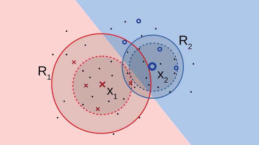
An example We make our discussion concrete
with an example. Figure 1 shows a two-dimensional
X space with labeled points L denoted as red
crosses and blue circles, unlabeled points as dots,
and the true labels as background color of the re-
gion. We show two rule-exemplar pairs: (x1 , y1 =
red, R1 ), (x2 , y2 = blue, R2 ) with bold boundaries.
Clearly, both rules R1 , R2 have over-generalized to
the wrong region. If we train a classifier with many
examples in H1 ∪ H2 wrongly labeled by rules, then Figure 1: Restricting over-generalized rules
even with a noise tolerant loss function like Zhang &
Sabuncu (2018), the classifier Pθ (y|x) might be misled. In contrast, what we hope to achieve is to
learn the Pjφ (rj |x) distribution using the limited labeled data and the overlap among the rules such
that Pr(rj |x) predicts a value of 0 for examples wrongly covered. Such examples are then excluded
from training Pθ . The dashed boundaries indicate the revised boundaries of Rj s that we can hope
to learn based on consensus on the labeled data and the set of rules. Even after such restriction, Rj s
are useful for training the classifier because of the unlabeled points inside the dashed regions that
get added to the labeled set.
2.1 H OW WE J OINTLY LEARN Pθ AND Pjφ
In general we will be provided with several rules with arbitrary overlap in the set of labeled L and
unlabeled examples U that they cover. Intuitively, we want the label distribution Pθ (y|x) to correctly
restrict the coverage distribution Pjφ (rj |x), which in turn can provide clean labels to instances in U
that can be used to train Pθ (y|x). We have two types of supervision in our setting. First, individually
for each of Pθ (y|x) and Pjφ (rj |x) we have ground truth values of y and rj for some instances. For
the Pθ (y|x) distribution, supervision on y is provided by the human labeled data L, and we use these
to define the usual log-likelihood as one term in our training objective:
X
max LL(θ) = max log Pθ (`i |xi ) (1)
θ θ
(xi ,`i )∈L
For learning the distribution Pjφ (rj |x) over the coverage variables, the only sure-shot labeled data
is that rji = 1 for any xi that is an exemplar of rule Rj and rji = 0 for any xi ∈ Hj whose label `i
is different from `j . For other labeled instances xi covered with rules Rj with agreeing labels, that
is `i = `j we do not strictly require that rji = 1. In the example above the corrected dashed red
boundary excludes a red labeled point to reduce its noise on other points. However, if the number
of labeled exemplars are too few, we regularize the networks towards more rule firings, by adding
a noise tolerant rji = 1 loss on the instances with agreeing labels. We use the generalized cross
entropy loss of Zhang & Sabuncu (2018).
X X
LL(φ) = log Pei φ (rei i = 1|xi ) + log Pjφ (rji = 0|xi )
(xi ,`i ,ei )∈L j:xi ∈Hj ∧ `i 6=`j
X (2)
− Generalized-XENT(Pjφ (rj |xi ), rji = 1)
j:xi ∈Hj ∧ `i =`j
Note for other instances xi in Rj ’s cover Hj , value of rji is unknown and latent. The second type of
supervision is on the relationship between rji and yi for each xi ∈ Hj . A rule Rj imposes a causal
constraint that when rji = 1, the label yi has to be `j .
rji = 1 =⇒ yi = `j ∀xi ∈ Hj (3)
We convert this hard constraint into a (log) probability of the constraint being satisfied under the
Pθ (y|x) and Pjφ (rj |x) distributions as:
log 1 − Pjφ (rj = 1|x)(1 − Pθ (`j |x)) (4)
Figure 2 shows a surface plot of the above log probability as a function of Pθ (`j |x) (shown
as axis P(y) in figure) and Pjφ (rj = 1|x) (shown as axis P(r) in figure) for a single rule.
3Published as a conference paper at ICLR 2020
Observe that likelihood drops sharply as
P (rj |x) is close to 1 but P (y = `j |x) is close
to zero. For all other values of these probabili-
ties the log-likelihood is flat and close to zero.
Specifically, when Pjφ predicts low values of
rj for a x, the log-likelihood surface is flat,
effectively withdrawing the (x, `j ) supervision
from training the classifier Pθ . Thus maximiz-
ing this likelihood provides a soft enforcement
of the constraint without unwanted biases. We
call this the negative implication loss.
We do not need to explicitly model the conflict
among rules, that is when an xi is covered by Figure 2: Negative implication loss
two rules Rj and Rk of differing labels (`j 6=
`k ), then both rji and rki cannot be 1. This is
because the constraint among pairs (yi , rji ) and (yi , rki ) as stated in Equation 3 subsumes this one.
During training we then seek to maximize the log of the above probability along with normal data
likelihood terms. Putting the terms in Equations 1, 2 and 4 together our final training objective is:
X
min −LL(θ) − LL(φ) − γ log(1 − Pjφ (rj = 1|x)(1 − Pθ (`j |x))) (5)
θ,φ
j;x∈Hj ∩U
We refer to our training loss as a denoised rule-label implication loss or ImplyLoss for short. The
LL(φ) term seeks to denoise rule coverage which then influence the y distribution via the implication
loss. We explored several other methods of enforcing the constraint among y and rj in the training
of the Pθ and Pjφ networks. Our method ImplyLoss consistently performed the best among several
methods we tried including the recent posterior regularization (Ganchev et al., 2010; Hu et al., 2016)
method of enforcing soft constraints and co-training (Blum & Mitchell, 1998).
Network Architecture Our network has three modules. (1) A shared embedding layer that pro-
vides the feature representation of the input. When labeled data is scarce, this will typically be a
pre-trained layer from a related task. The embedding module is task-specific and is described in
the experiment section. (2) A classification network that models Pθ (y|x) with parameters θ. The
embedding of an input x is passed through multiple non-linear layers with ReLU activation, a last
linear layer followed by Softmax to output a distribution over the class labels. (3) A rule network
that models Pjφ (rj = 1|x) whose parameters φ are shared across all rules. The input to the network
is rule-specific and concatenates the embedding of the input instance x, and a one-hot encoding of
the rule id ’j’. The input is passed through multiple non-linear layers with ReLU activation before
passing through a Sigmoid activation which outputs the probability Pjφ (rj = 1|x).
Inference During prediction, joint inference over the label y and coverage variables rj provides
slight gains over depending solely on Pθ (y|x). For any test example x, consider the set of rules
G covering x such that Pjφ (1|x) > 0.5. Probabilities from the label and coverage variables are
combined to obtain a score s(y) for each label y as:
P
Rj ∈G δ(`j = y)Pjφ (1|x) + δ(`j 6= y)Pjφ (0|x)
s(y|x) = Pθ (y|x) + (6)
|G|
The above can be viewed as a soft voting over the trained classifier Pθ and labels provided by rules
with uncertain coverage. Because we also learned to denoise rules along with training the classifier,
the labels assigned by the rules have higher precision than original rules.
3 E XPERIMENTS
We compare our training algorithms against simple baselines, existing error-tolerant learning algo-
rithms, and existing constraint-based learning in deep networks.
We evaluate across five datasets spanning three task types: text classification, sequence labeling,
and record classification. We augment the datasets with rules, that we obtained manually in three
4Published as a conference paper at ICLR 2020
Dataset |L| |U | #Rules %Cover Precision %Conflict Avg #Rules |Valid| |Test|
|Hj | Per In-
stance
Question 68 4884 68 95 63.8 22.5 124 1.8 500 500
MIT-R 1842 64888 15 14 80.7 2.5 634 1.1 4091 14256
SMS 69 4502 73 40 97.3 0.6 31 1.3 500 500
YouTube 100 1586 10 87 78.6 30.2 258 1.9 120 250
Census 83 10000 83 100 84.1 27.5 540 4.5 5561 16281
Table 1: Statistics of datasets and their rules. %Cover is fraction of instances in U covered by at least one rule.
Precision refers to micro precision of rules. Conflict denotes the fraction of instances covered by conflicting
rules among all the covered instances. Avg |Hj | is average cover size of a rule in U . Rules Per Instance is
average number of rules covering an instance in U .
cases, from pre-existing public sources in one case, and automatically in another. Table 1 presents
statistics summarizing the datasets and rules. A brief description of each appears below.
Question Classification (Li & Roth, 2002): This is a TREC-6 dataset to classify a question to
one of six categories: {Abbreviation, Entity, Description, Human, Location,
Numeric-value}. The training set has 5452 instances which are split as 68 for L, 500 for val-
idation, and the remaining as U . Each example in L is generalized as a rule represented by a
regular expression. E.g. After labeling How do you throw a housewarming party ?
as Description we define a rule
(how|How|what|What)(does|do|to|can).∗ → Description.
More rules in Table 4 of supplementary. Although, creating such 68 generalised rules required
90 minutes, the generalizations cover 4637 instances in U , almost two orders of magnitude more
instances than in L! On an average each of our rule covered 124 instances (|Hj | column in Table 1).
But the precision of labels assigned by rules was only 63.8%. 22.5% of covered instances had an
inter-rule conflict, demonstrating noise in the rule labelings. Accuracy is used as the performance
metric.
MIT-R1 (Liu et al., 2013): This is a slot-filling task on sentences about restaurant search and the
task is to label each token as one of {Location, Hours, Amenity, Price, Cuisine,
Dish, Restaurant Name, Rating, Other}. The training data is randomly split into 200
sentences (1842 tokens) as L, 500 sentences (4k tokens) as validation and remaining 6.9k sen-
tences (64.9k tokens) as U . We manually generalize 15 examples in L. E.g. After inspecting
the sentence where can i get the highest rated burger within ten miles
and labeling highest rated as Rating, we provide the rule:
. ∗ (highly|high|good|top|highest)(rate|rating|rated).∗ → Rating
to the matched positions. More examples in Table 7 of supplementary. Although, creating 15
generalizing rules took 45 minutes of annotator effort, the rules covered roughly 9k tokens in U . F1
metric is used for evaluation on the default test set of 14.2k tokens over 1.5k sentences.
SMS Spam Classification (Almeida et al., 2011): This dataset contains 5.5k text messages labeled
as spam/not-spam, out of which 500 were held out for validation and 500 for testing. We manually
generalized 69 exemplars to rules. Remaining examples go in the U set. The rules here check
for presence of keywords or phrases in the SMS .* guaranteed gift .* → spam. A rule
covers 31 examples on an average and has a precision of 97.3%. However, in this case only 40% of
the unlabeled set is covered by a rule. We report F1 here since class is skewed. More examples in
Table 5 of supplementary.
Youtube Spam Classification (Alberto et al., 2015): Here the task is to classify comments on
YouTube videos as Spam or Not-Spam. We obtain this from Snorkel’s Github page2 , which provides
10 labeling functions which we use as rules, an unlabeled train set which we use as U , a labeled dev
set to guide the creation of their labeling functions which we use as L, and labeled test and validation
sets which we use in the same roles. Their labeling functions have a large coverage (258 on average),
and a precision of 78.6%.
Census Income (Dua & Graff, 2019): This UCI dataset is extracted from the 1994 U.S. census. It
lists a total of 13 features of an individual such as age, education level, marital status, country of
1
groups.csail.mit.edu/sls/downloads/restaurant/
2
https://github.com/snorkel-team/snorkel-tutorials/tree/master/spam
5Published as a conference paper at ICLR 2020
Datasets
Methods
Question MIT-R YouTube SMS Census
(Accuracy) (F1) (Accuracy) (F1) (Accuracy)
Majority (No parameters trained) 60.9 (0.7) 40.9 (0.1) 82.2 (0.9) 48.4 (1.2) 80.1 (0.1)
Only-L 72.9 (0.6) 73.5 (0.3) 90.9 (1.8) 89.0 (1.6) 79.4 (0.5)
L+Umaj - 1.4 (1.5) + 0.0 (0.3) + 0.8 (1.9) + 3.5 (1.2) + 0.9 (0.1)
Noise-tolerant (Zhang et al., 2018) - 0.5 (1.1) + 0.0 (0.2) + 1.7 (1.1) + 2.9 (1.2) + 1.0 (0.2)
L2R (Ren et al., 2018b) + 0.3 (2.1) - 15.4 (1.0) + 2.5 (0.5) + 2.3 (0.8) + 2.9 (0.3)
L+Usnorkel (Ratner et al., 2016) - 0.7 (3.0) + 0.0 (0.2) + 2.7 (0.7) + 3.5 (1.3) + 1.0 (0.4)
Snorkel-Noise-Tolerant - 1.4 (1.6) + 0.0 (0.3) + 2.0 (0.7) + 2.7 (1.5) + 0.2 (0.5)
Posterior Reg. (Hu et al., 2016) - 0.8 (1.0) - 0.1 (0.4) - 2.9 (1.9) + 1.8 (1.5) - 0.8 (0.5)
ImplyLoss (Ours) + 11.7 (1.5) + 0.8 (0.3) + 3.2 (1.1) + 4.2 (1.0) + 1.7 (0.2)
Table 2: Comparison of ImplyLoss (our method) with various methods (described in Section 3.1) on five
different datasets. The numbers reported for all methods after the double-line are gains over the baseline (Only-
L) that does not use rules at all. Higher is better. NOTE: Numbers in brackets represent standard deviation of
the original accuracy and not of gains.
origin etc. The primary task on it is binary classification - whether a person earns more than $50K
or not. The train data consists of 32563 records. We choose 83 random data points as L, 10k points
as U and 5561 points as validation data. For this case we created the rules synthetically as follows:
We hold out disjoint 16k random points from the training dataset as a proxy for human knowledge
and extract a PART decision list (Frank & Witten, 1998) from it as our set of rules. We retain only
those rules which fire on L.
Network Architecture Since our labeled data is small we depend on pre-trained resources. As
the embedding layer we use a pretrained ELMO (Peters et al., 2018) network where 1024 dimen-
sional contextual token embeddings serve as representations of tokens in the MIT-R sentences, and
their average serve as representation for sentences in Question and SMS dataset. Parameters of the
embedding network are held fixed during training. For sentences in the YouTube dataset, we use
Snorkel’s2 architecture of a simple bag-of-words feature representation marking the frequent uni-
grams and bi-grams present in a sentence using a few-hot vector. For the Census dataset categorical
features are represented as one hot vectors, while real valued features are simply normalized. For
MIT-R, Question and SMS both classification and rule-weight network contain two 512 dimensional
hidden layers with ReLU activation. For Census, both the networks contain two 256 dimensional
hidden layers with ReLU activation. For YouTube, the classifier network is a simple logistic re-
gression like in Snorkel’s code. The rule network has one 32-dimensional hidden layer with ReLU
activation.
Each reported number is obtained by averaging over ten random initializations. Whenever a method
involved hyper-parameters to weigh the relative contribution of various terms in the objective, we
used a validation dataset to tune the value of the hyper-parameter. Hyperparameters used are pro-
vided in Section C of supplementary.
3.1 C OMPARISON WITH DIFFERENT METHODS
In Table 2 we compare our method with the following alternatives on each of the five datasets:
Majority: that predicts via majority vote among the rules that cover an instance. This baseline
indicates the stand-alone quality of rules, no network is learned here. Ties are broken arbitrarily for
class-balanced datasets or by using a default class. Table 2, shows that the accuracy of majority is
quite poor indicating either poor precision or poor coverage of the rule sets.3 .
Only-L: Here we train the classifier Pθ (y|x) only on the labeled data L using the standard cross-
entropy loss (Equation 1). Rule generalisations are not utilized at all in this case. We observe
in Table 2 that even with the really small labeled set we used for each dataset, the accuracy of a
classifier learned with clean labeled data is much higher than noisy majority labels of rules. We
consider this method as our baseline and report the gains on remaining methods.
3
Only for the Census dataset the relative accuracy is high because the rules were obtained synthetically
through a rule-learning algorithm on a very large labeled dataset to serve as a proxy for a human’s generaliza-
tion.
6Published as a conference paper at ICLR 2020
L+Umaj: Next we train the classifier on L along with Umaj obtained by labeling instances in U with
the majority label among the rules applicable to the instance. Loss corresponding to the examples
labeled by rules is weighted as follows:
X X
min − log Pθ (`j |xj ) + γ − log Pθ (yj |xj ) (7)
θ
(xj ,`j )∈L (xj ,yj )∈Umaj
The row corresponding to L+Umaj in Table 2 provides the gains of this method over Only-L. We
observe gains with the noisily labeled U in three out of the five cases.
Noise-tolerant: Since labels in Umaj are noisy, we next use Zhang & Sabuncu (2018)’s noise tolerant
generalized cross entropy loss on them with regular cross-entropy loss on the clean L as follows:
q
X X (1 − Pθ (yj |x))
min − log Pθ (`j |xj ) + γ (8)
θ q
(xj ,`j )∈L (xj ,yj )∈Umaj
Parameter q ∈ [0, 1] controls the noise tolerance which we tune as a hyper-parameter. We observe
that in three cases minimizing the above objective improves beyond L+Umaj validating that noise-
tolerant loss functions can be useful for learning from noisy labels on Umaj .
Learning to Reweight (L2R) (Ren et al., 2018b): is a recent method for training with a mix of
clean and noisy labeled data. They train the classifier by meta-learning to re-weight the loss on
the noisily labelled instances (Umaj ) with the help of the clean examples (L). This method provides
significant accuracy gains over Only-L in three out the five datasets. However, it fails in the multi-
class classification task of slot-filling which has a very high class imbalance and rules of smaller
coverage.
All the above methods employ no extra parameters to denoise or weight individual rules. We next
compare with a number of methods that do.
L+Usnorkel: This method replaces Majority-based consensus with Snorkel’s generative model
(Ratner et al., 2016) that assigns weights to rules and labels examples in U . Thereafter we use
the same approach as in L+Umaj with just Snorkel’s soft-labels instead of Majority on U . We also
compare with using noise-tolerant loss on U labeled by Snorkel (Eqn:8) which we call Snorkel-
Noise-Tolerant. Like previous methods, both of these methods provide improvements over Only-L
on three of the five datasets where the rules are less noisy. L+Usnorkel performs slightly better than
Noise-Tolerant on Umaj .
We next compare with a method that simultaneously learns two sets of networks Pθ and Pjφ like
ours but with different loss function and training schedule.
Posterior Regularization (PR): This method proposed in Hu et al. (2016) also treats rules as soft-
constraints and has been used for training neural networks for structured outputs. They use Ganchev
et al. (2010)’s posterior regularization framework to train the two networks in a teacher-student
setup. We adapt the same framework and get a procedure as follows: The student proposes a dis-
tribution over y and rj s using current Pθ and Pjφ , the teacher uses the constraint in Eq 3 to revise
the distributions so as to minimize the probability of violations, the student updates parameters θ
and φ to minimize KL distance with the revised distribution. The detailed formulation appear in the
Section A of supplementary. We find that this method is no better than Only-L in most of the cases
and worse than the noise-tolerant method that does not train extra φ parameters.
ImplyLoss(Ours): Overall our approach of training with denoised rule-label implication loss pro-
vides much better accuracy than all the above eight methods and we get consistent gains over Only-L
on all datasets. On the Question dataset we get 11.7 points gain over Only-L whereas the best gain
by existing method was 0.3. A useful property of our method compared to the PR method above
is that the training process is simple and fits into the batch stochastic gradient training template. In
contrast, PR requires special alternating computations. We next perform a number of diagnostics
experiments to explain the reasons for the superior performance of our method.
7Published as a conference paper at ICLR 2020
Diagnostics: Effectiveness of learning true Old precision Denoised Precision Percent Suppressed
coverage via Pjφ An important part of our 99
method is the rule-specific denoising learned 88
via the Pjφ network. In the chart alongside we 77
plot the original precision of rules on the test 66
data, and the precision after suppressing those 55
rule labelings where Pjφ (rj |x) predicts 0 in- 44
stead of 1. Observe now that the precision is 33
22
more than 91% on all datasets. For the Ques-
11
tion dataset, the precision jumped from 64% to
0
98%. The percentage of labelings suppressed Question MIT-R YouTube SMS Census
(shown by the dashed line) is higher on datasets Figure 3: Rule-specific denoising by our method.
with noisier rules (e.g. compare Question and
SMS). This shows that Pjφ is able to denoise rules by capturing the distribution of the latent true
coverage variables with the limited LL(φ) loss and indirectly via the implication loss.
Effect of rule precision Rules in the Census
Ours L2R
dataset are of higher quality in terms of preci-
83
sion as well as coverage. Superior performance
of the L2R method on this dataset motivated us 81
to inspect how well our method performs on Accuracy
79
the same dataset in the absence of high preci-
sion rules. We created four new versions of the 77
rule sets by successively removing high preci-
sion rules from the original rule set. We ob- 75
56 66 71 75 83
serve that our method performs better than L2R
when rules have low precision. Because Imply- Rule Precision
Loss denoises rules, it is better able to handle Figure 4: Effect of rule precision
low-precision rules.
Role of Exemplars in Rules We next evaluate the importance of the exemplar-rule pairs in
learning the Pjφ and Pθ networks. The exemplars of a rule give an interesting new form of
supervision about an instance where a labeling rule must fire. To evaluate the importance of this
supervision, we exclude the rj = 1 likelihood on rule-exemplar pairs from LL(φ), that is, the
first term in Equation 2 is dropped. In the table below we see that performance of ImplyLoss
usually drops when the exemplar-rule supervision is removed. Interestingly, even after this drop, the
performance of ImplyLoss surpasses most of the methods in Table 2 indicating that even without
exemplar-rule pairs our training objective is effective in learning from rules and labeled instances.
Question MIT-R SMS Census
rj = 1 for rule-exemplar pairs 84.5 (1.5) 73.7 (0.3) 93.2 (1.0) 81.0 (0.2)
No rj = 1 for rule-exemplar pairs 83.8 (0.7) 73.5 (0.5) 93.5 (1.2) 80.8 (0.3)
Table 3: Effect of removing rule-exemplar supervision from LL(φ)
Effect of increasing labeled data L We in-
Ours Posterior Reg. L+Usnorkel Only-L
crease L while keeping the number of rules 90
fixed on the Question dataset. In the attached
plot we see the accuracy of our method (Imply- 85
Loss) against Only-L, L+Usnorkel and Poste-
Accuracy
80
rior Reg. We observe the expected trend that
the gap between the method narrows as labeled 75
data increases.
70
68 200 400 600 800
4 R ELATED W ORK Size of L
Learning from noisily labeled data has been
Figure 5: Effect of increasing labeled data
extensively studied in settings like crowd-
sourcing. One category of these algorithms
upper-bound the loss function to make it robust to noise. These include methods like MAE (Ghosh
8Published as a conference paper at ICLR 2020
et al., 2017), Generalized Cross Entropy (CE)(Zhang & Sabuncu, 2018), and Ramp loss (Collobert
et al., 2006). Most of these assume that noise is independent of the input given the true label. In our
model noise is systematic and instance-dependent.
A second category assume that a small clean dataset is available along with noisily labeled data.
This is also true in our case, and we compared with a state of the art method in that category Ren
et al. (2018b) that chooses a descent direction that aligns with a clean validation set using meta-
learning. Others in this category include: Shen & Sanghavi (2019)’s method of iteratively selecting
examples with smallest loss, and Veit et al. (2017)’s method of learning a separate network to trans-
form noisy labels to cleaned ones which are used to impose a cross-entropy loss on Pθ (y|x). In
contrast, we perform rule-specific cleaning via latent coverage variables and a flexible implication
loss which withdraws y supervision when Pjφ (rji |x) assumes low values. Another way of relat-
ing clean and noisy labels is via an instance-independent confusion matrix learned jointly with the
classifier (Khetan et al., 2018; Goldberger & Ben-Reuven, 2016; Han et al., 2018b;a). These works
assume that the confusion matrix is instance independent, which does not hold for our case. Tanaka
et al. (2018) uses confidence from the classifier to eliminate noise but they need to ensure that the
network does not memorize noise. Our learning setup also has the advantage of extracting confi-
dence from a different network. There is growing interest in integrating logical rules with labeled
examples for training networks, specifically for structured outputs (Manhaeve et al., 2018; Xu et al.,
2018; Fischer et al., 2019; Sun et al., 2018; Ren et al., 2018a). Xu et al. (2018); Fischer et al. (2019)
convert rules on output nodes of network, to (almost differentiable) loss functions during training.
The primary difference of these methods from ours is that they assume that rules are correct whereas
we assume them to be noisy. Accordingly, we simultaneously correct the rules and use them to
improve the classifier, whereas they use the rules as-is to train the network outputs.
A well-known framework for working with soft rules is posterior regularization (Ganchev et al.,
2010) which is used in Hu et al. (2016) to train deep structured output networks while harnessing
logic rules. Ratner et al. (2016) works only with noisy rules treating them as black-box labeling
functions and assigns a linear weight to each rule based on an agreement objective. Our learn-
ing model is more powerful that attempts to learn a non-linear network to restrict rule boundaries
rather than just weight their outputs. We presented a comparison with both these approaches in the
experimental section, and showed superior performance.
To the best of our knowledge, our proposed paradigm of coupled rule-exemplar supervision is novel,
and our proposed training algorithm is able to harness them in ways not possible by existing frame-
works for learning from rules or noisy supervision.
5 C ONCLUSION
We proposed a new rule-exemplar model for collecting human supervision to combine the scalability
of top-level rules with the quality of instance-level labels. We show that such supervision is natural
since humans typically inspect examples to code rules. Furthermore, such coupled examples provide
supervision on correct firing of rules which help to denoise rules. We propose to train the classifier
while jointly denoising rules via latent coverage variables imposing a soft-implication constraint
on the true label. Empirically on five datasets we show that our training algorithm that performs
rule-specific denoising is better than generic noise-tolerant learning. In future we plan to deploy this
framework on other applications where human supervision is a scarce resource.
Reproducibility Code and Data for the experiments available at
https://github.com/awasthiabhijeet/Learning-From-Rules
Acknowledgements We thank the anonymous reviewers for their constructive feedback on this
work. This research was partly sponsored by a Google India AI/ML Research Award and partly
by the IBM AI Horizon Networks - IIT Bombay initiative. Abhijeet is supported by Google PhD
Fellowship in Machine Learning.
9Published as a conference paper at ICLR 2020
R EFERENCES
Túlio C Alberto, Johannes V Lochter, and Tiago A Almeida. Tubespam: Comment spam filtering
on youtube. In 2015 IEEE 14th International Conference on Machine Learning and Applications
(ICMLA), pp. 138–143. IEEE, 2015.
Tiago A Almeida, José Marı́a G Hidalgo, and Akebo Yamakami. Contributions to the study of
sms spam filtering: new collection and results. In Proceedings of the 11th ACM symposium on
Document engineering, pp. 259–262. ACM, 2011.
Douglas E. Appelt, Jerry R. Hobbs, John Bear, David J. Israel, and Mabry Tyson. Fastus: A finite-
state processor for information extraction from real-world text. In IJCAI, pp. 1172–1178, 1993.
Stephen H. Bach, Daniel Rodriguez, Yintao Liu, Chong Luo, Haidong Shao, Cassandra Xia, Souvik
Sen, Alexander Ratner, Braden Hancock, Houman Alborzi, Rahul Kuchhal, Christopher Ré, and
Rob Malkin. Snorkel drybell: A case study in deploying weak supervision at industrial scale. In
Proceedings of the 2019 International Conference on Management of Data, SIGMOD Conference
2019, Amsterdam, The Netherlands, June 30 - July 5, 2019., pp. 362–375, 2019.
Avrim Blum and Tom Mitchell. Combining labeled and unlabeled data with co-training. In COLT,
1998.
R. Collobert, F. Sinz, J. Weston, and L. Bottou. Trading convexity for scalability. In ICML 2006,
2006.
Hamish Cunningham. Gate: A framework and graphical development environment for robust nlp
tools and applications. In Proc. 40th Annual Meeting of the Association for Computational Lin-
guistics (ACL 2002), pp. 168–175, 2002.
Arthur P Dempster, Nan M Laird, and Donald B Rubin. Maximum likelihood from incomplete data
via the em algorithm. Journal of the Royal Statistical Society: Series B (Methodological), 39(1):
1–22, 1977.
Jacob Devlin, Ming-Wei Chang, Kenton Lee, and Kristina Toutanova. Bert: Pre-training of deep
bidirectional transformers for language understanding. arXiv preprint arXiv:1810.04805, 2018.
Dheeru Dua and Casey Graff. UCI machine learning repository, 2019. URL http://archive.ics.uci.
edu/ml.
Marc Fischer, Mislav Balunovic, Dana Drachsler-Cohen, Timon Gehr, Ce Zhang, and Martin
Vechev. DL2: Training and querying neural networks with logic. In Proceedings of the 36th
International Conference on Machine Learning, pp. 1931–1941, 2019.
Eibe Frank and Ian H. Witten. Generating accurate rule sets without global optimization. In J. Shav-
lik (ed.), Fifteenth International Conference on Machine Learning, pp. 144–151. Morgan Kauf-
mann, 1998.
Kuzman Ganchev, Jennifer Gillenwater, Ben Taskar, et al. Posterior regularization for structured
latent variable models. Journal of Machine Learning Research, 11(Jul):2001–2049, 2010.
Aritra Ghosh, Himanshu Kumar, and PS Sastry. Robust loss functions under label noise for deep
neural networks. In Thirty-First AAAI Conference on Artificial Intelligence, 2017.
Garrett B. Goh, Charles Siegel, Abhinav Vishnu, and Nathan Hodas. Using rule-based labels for
weak supervised learning: A chemnet for transferable chemical property prediction. In Proceed-
ings of the 24th ACM SIGKDD International Conference on Knowledge Discovery & Data
Mining, KDD ’18, 2018.
Jacob Goldberger and Ehud Ben-Reuven. Training deep neural-networks using a noise adaptation
layer. 2016.
Bo Han, Jiangchao Yao, Gang Niu, Mingyuan Zhou, Ivor Tsang, Ya Zhang, and Masashi Sugiyama.
Masking: A new perspective of noisy supervision. In Advances in Neural Information Processing
Systems, pp. 5841–5851, 2018a.
10Published as a conference paper at ICLR 2020
Bo Han, Quanming Yao, Xingrui Yu, Gang Niu, Miao Xu, Weihua Hu, Ivor Tsang, and Masashi
Sugiyama. Co-teaching: Robust training of deep neural networks with extremely noisy labels. In
Advances in Neural Information Processing Systems 31, pp. 8536–8546. 2018b.
Zhiting Hu, Xuezhe Ma, Zhengzhong Liu, Eduard Hovy, and Eric Xing. Harnessing deep neural
networks with logic rules. In Proceedings of the 54th Annual Meeting of the Association for
Computational Linguistics (Volume 1: Long Papers), August 2016.
Dongyeop Kang, Tushar Khot, Ashish Sabharwal, and Eduard Hovy. Adventure: Adversarial train-
ing for textual entailment with knowledge-guided examples. In Proceedings of the 56th Annual
Meeting of the Association for Computational Linguistics (Volume 1: Long Papers). Association
for Computational Linguistics, 2018.
Ashish Khetan, Zachary C. Lipton, and Anima Anandkumar. Learning from noisy singly-labeled
data. In International Conference on Learning Representations, 2018. URL https://openreview.
net/forum?id=H1sUHgb0Z.
Xin Li and Dan Roth. Learning question classifiers. In Proceedings of the 19th international confer-
ence on Computational linguistics-Volume 1, pp. 1–7. Association for Computational Linguistics,
2002.
Jingjing Liu, Panupong Pasupat, Yining Wang, Scott Cyphers, and Jim Glass. Query understand-
ing enhanced by hierarchical parsing structures. In 2013 IEEE Workshop on Automatic Speech
Recognition and Understanding, pp. 72–77. IEEE, 2013.
Robin Manhaeve, Sebastijan Dumancic, Angelika Kimmig, Thomas Demeester, and Luc De Raedt.
Deepproblog: Neural probabilistic logic programming. In Advances in Neural Information Pro-
cessing Systems 31, pp. 3749–3759. 2018.
Arghya Pal and Vineeth N. Balasubramanian. Adversarial data programming: Using gans to relax
the bottleneck of curated labeled data. In 2018 IEEE Conference on Computer Vision and Pattern
Recognition, CVPR 2018, Salt Lake City, UT, USA, June 18-22, 2018, pp. 1556–1565, 2018.
Matthew E Peters, Mark Neumann, Mohit Iyyer, Matt Gardner, Christopher Clark, Kenton Lee, and
Luke Zettlemoyer. Deep contextualized word representations. arXiv preprint arXiv:1802.05365,
2018.
Alexander J Ratner, Christopher M De Sa, Sen Wu, Daniel Selsam, and Christopher Ré. Data pro-
gramming: Creating large training sets, quickly. In Advances in Neural Information Processing
Systems 29. 2016.
Hongyu Ren, Russell Stewart, Jiaming Song, Volodymyr Kuleshov, and Stefano Ermon. Learning
with weak supervision from physics and data-driven constraints. AI Magazine, 39(1):27–38,
2018a.
Mengye Ren, Wenyuan Zeng, Bin Yang, and Raquel Urtasun. Learning to reweight examples for
robust deep learning. arXiv preprint arXiv:1803.09050, 2018b.
Yanyao Shen and Sujay Sanghavi. Learning with bad training data via iterative trimmed loss mini-
mization. In Proceedings of the 36th International Conference on Machine Learning, pp. 5739–
5748, 2019.
Chen Sun, Abhinav Shrivastava, Saurabh Singh, and Abhinav Gupta. Revisiting unreasonable ef-
fectiveness of data in deep learning era. In IEEE International Conference on Computer Vision,
ICCV 2017, Venice, Italy, October 22-29, 2017, pp. 843–852, 2017.
Haitian Sun, William W Cohen, and Lidong Bing. Semi-supervised learning with declaratively
specified entropy constraints. In Advances in Neural Information Processing Systems 31, pp.
4425–4435. 2018.
Daiki Tanaka, Daiki Ikami, Toshihiko Yamasaki, and Kiyoharu Aizawa. Joint optimization frame-
work for learning with noisy labels. In Proceedings of the IEEE Conference on Computer Vision
and Pattern Recognition, pp. 5552–5560, 2018.
11Published as a conference paper at ICLR 2020
Michael Henry Tessler and Noah D. Goodman. The language of generalization. Psychological
Review, 126(3):395–436, 2019.
Andreas Veit, Neil Alldrin, Gal Chechik, Ivan Krasin, Abhinav Gupta, and Serge Belongie. Learning
from noisy large-scale datasets with minimal supervision. In Proceedings of the IEEE Conference
on Computer Vision and Pattern Recognition, pp. 839–847, 2017.
Jingyi Xu, Zilu Zhang, Tal Friedman, Yitao Liang, and Guy Van den Broeck. A semantic loss
function for deep learning with symbolic knowledge. In Proceedings of the 35th International
Conference on Machine Learning, pp. 5502–5511, 2018.
Zhilu Zhang and Mert Sabuncu. Generalized cross entropy loss for training deep neural networks
with noisy labels. In Advances in Neural Information Processing Systems 31. 2018.
12Published as a conference paper at ICLR 2020
Supplementary Material: Learning from
Rules Generalizing Labeled Exemplars
A P OSTERIOR R EGULARIZATION M ETHOD
We model a joint distribution Q(y, r1 , . . . , rn |x) to capture the interaction among the label random
variable y and coverage random variables r1 , . . . , rn of any instance x. We use r to compactly
represent r1 , . . . , rn . Strictly speaking, when a rule Rj does not cover x, the rj is not a random
variable and its value is pinned to 0 but we use this fixed-tuple notation for clarity. The random
variables rj and y impose a constraint on the joint distribution Q: for a x ∈ Hj when rj = 1, the
label y cannot be anything other than `j .
rj = 1 =⇒ y = `j ∀x ∈ Hj (9)
We can convert P this into a soft constraint on the marginals of the distribution Q by stating the
probability of y6=`j Q(y, rj = 1|x) should be small.
X X X
min Q(y, rj = 1|x) (10)
Q
j x∈Hj y6=`j
The singleton marginals of Q along the y and rj variables are tied to the Pθ and Pjφ (rj |x) we seek
to learn. A network with parameters θ models the classifier Pθ (y|x), and a separate network with φ
variables (shared across all rules) learns the Pjφ (rj |x) distribution. The marginals of joint Q should
match these trained marginals and we use a KL term for that:
X X
min KL(Q(y|x); Pθ (y|x)) + KL(Q(rj |x); Pjφ (rj |x)) (11)
Q,θ,φ
x∈U ∪L j:x∈Hj
We call the combined KL term succinctly as KL(Q, Pθ ) + KL(Q, Pφ ).
Further the Pθ and Pjφ distributions should maximize the log-likelihood on their respective labeled
data as provided in Equation 1 and Equation 2 respectively.
Putting all the above objectives together with hyper-parameters α > 0, λ > 0 we get our final
objective as:
X X X
min −α(LL(θ) + LL(φ)) + KL(Q, Pθ ) + KL(Q, Pφ ) + λ Q(y, rj = 1|x) (12)
Q,θ,φ
j x∈Hj y6=`j
We show in Section A.1 that this gives rise to the solution for Q in terms of Pθ , Pjφ and alternately
for Pθ , Pjφ in terms of Q as follows.
Y
Q(y, r|x) ∝ Pθ (y|x) Pjφ (rj |x)e−λδ(y6=`j ∧rj =1) (13)
j:x∈Hj
where δ(y 6= `j ∧ rj = 1) is an indicator function that is 1 when the constraint inside holds, else it
is 0. Computing marginals of the above using straight-forward message passing techniques we get:
Y
Q(y|x) ∝ Pθ (y|x) (Pjφ (1|x)e−λδ(y6=`j ) + Pjφ (0|x)) (14)
j:x∈Hj
X Y
Q(rk = 1|x) ∝ Pkφ (1|x) e−λδ(y6=`k ) Pθ (y|x) (Pjφ (1|x)e−λδ(y6=`j ) + Pjφ (0|x))
y j6=k,x∈Hj
(15)
Thereafter, we solve for θ and φ in terms of a given Q as
XX X X
min −LL(θ) − LL(φ) − γ Q(y|xi ) log Pθ (y|xi ) + Q(rj |xi ) log Pjφ (rj |xi )
θ,φ
xi ∈U y∈Y j:xi ∈Hj rj ∈{0,1}
(16)
Here, γ = α1 . This gives rise to an alternating optimization algorithm as in the posterior regular-
ization framework of Ganchev et al. (2010). We initialize θ and φ randomly. Then in a loop, we
perform the following two steps alternatively much like the EM algorithm (Dempster et al., 1977).
13Published as a conference paper at ICLR 2020
Q Computation step: Here we compute marginals Q(y|x) and Q(rj |x) from current Pθ and Pjφ
using Equations 14 and 15 respectively for each x in a batch. This computation is straight-forward
and does not require any neural optimization. We can interpret the Q(y|x) as a small correction of
the Pθ (y|x) so as to align better with the constraints imposed by the rules in Equation 3. Likewise
Q(rj |x) is an improvement of current Pjφ s in the constraint preserving direction. For example, the
expected rj values might be reduced for an instance if its probability of y being `j is small.
Parameter update step: We next reoptimize the θ and φ parameters to match the corrected Q
distribution as shown in Equation 16. This is solved using standard stochastic gradient techniques.
The Q terms can just be viewed as weights at this stage which multiply the loss or label likelihood.
A pseudocode of our overall training algorithm is described in Algorithm 1.
Algorithm 1 Our Joint Training Algorithm using Posterior Regularization
Input: L, U
Initialize parameters θ, φ randomly
for a random training batch from U ∪ L do
Obtain Pθ (y|x) from the classification network.
Obtain Pjφ (rj |x)j∈[n] from the rule-weight network.
Calculate Q(y|x) using Eqn 14 and Q(rj |x)j∈[n] using Eqn 15.
Update θ and φ by taking a step in the direction to minimize the loss in Eqn 16.
end for
Output: θ , φ
A.1 P ROOF : A LTERNATING SOLUTION FOR O PTIMIZATION O BJECTIVE IN E QN 12
P
Treat each Q(y, r) as an optimization variable with the constraint that y,r Q(y, r) = 1. We express
this constraint with a Langrangian multiplier η in the objective. Also, define a distribution
Y
Pθ,φ (y, r|x) = Pθ (y|x) Pjφ (rj |x)
j:x∈Hj
It is easy to verify that the KL terms in our objective 12 can be collapsed as KL(Q; Pθ,φ ). The
rewritten objective (call it F (Q, θ, φ) ) is now:
X
−α(LL(θ) + LL(φ)) + KL(Q(y, r|x), Pθ,φ (y, r|x))
x
X X X X (17)
+λ Q(y, rj = 1|x) + η(1 − Q(v, r))
j x∈Hj y6=`j y,r
∂F
Next we solve for ∂Q(y,r) = 0 after expressing the marginals in their expanded forms: e.g.
P
Q(y, rj |x) = r1 ,...,rj−1 ,rj+1 ,...,rn Q(y, r1 , . . . , rn |x). This gives us
∂F
= log Q(y, r) − log Pθ,φ (y, r|x)
∂Q(y, r)
P
+ j:x∈Hj λδ(y 6= `j , rj = 1) + η + 1
Equating it to zero and substituting for Pθ,φ we get the solution for Q(y, r) in Equation 13.
The proof for the optimal Pθ and Pjφ while keeping Q fixed in Equation 17 is easy and we skip
here.
14Published as a conference paper at ICLR 2020
B L IST OF RULES
We provide a list of rules for each task type.
Rule Example Class
( |ˆ)(where)[ˆ\w]* (\w+ ){0,1} Where is Trinidad ? Location
(was|is)[ˆ\w]*( |\$)
( |ˆ)(which|what)[ˆ\w]* (\w+ ){0,1} What book is the follow-up Entity
(play|game|movie|book)[ˆ\w]*( |$) to Future Shock ?
( |ˆ)(what)[ˆ\w]* (\w+ ){0,1} Of children between the Numeric
(part|division|ratio|percentage) ages of two and eleven ,
[ˆ\w]*( |$) what percentage watch “
The Simpsons ” ?
( |ˆ)(who|who)[ˆ\w]* (\w+ ){0,1} Who invented volleyball ? Human
(found|discovered|made|built
|build|invented)[ˆ\w]*( |$)
Table 4: Sample rules for TREC Question Classification. Rule fires if the regex matches
Rule Example Class
( |ˆ)(free)[ˆ\w]* Free video camera phones with Spam
([ˆ\s]+ )*(price)[ˆ\w]* Half Price line rental for 12 mths
([ˆ\s]+ )*(call)[ˆ\w]*( |$) and 500 cross ntwk mins 100 txts.
Call MobileUpd8 08001950382 or
Call2OptOut/674
( |ˆ)(guranteed)[ˆ\w]* ([ˆ\s]+ )* Great News! Call FREEFONE Spam
(gift\.|gift)[ˆ\w]*( |$) 08006344447 to claim your guaran-
teed å£1000 CASH or å£2000 gift.
( |ˆ)(can’t)[ˆ\w]* sry can’t talk on phone, with parents NotSpam
(\w+ ){0,1}(talk)[ˆ\w]*( |$)
( |ˆ)(that’s)[ˆ\w]* Yeah, that’s fine! It’s å£6 to get in, NotSpam
(\w+ ){0,1}(fine!|fine)[ˆ\w]*( |$) is that ok?
Table 5: Sample rules for Spam Classification. Rule fires if the regex matches
Rules Class
capital-gain > 6849 > 50K
education-num > 12 AND > 50K
marital-status = Never-married AND
native-country = United-States AND
occupation = Exec-managerial
marital-status = Separated AND ≤ 50K
hours-per-week ≤ 41
education-num ≤ 12 AND ≤ 50K
native-country = United-States AND
age ≤ 30
Table 6: Sample rules for census dataset. Rule fires if all clauses are True
15Published as a conference paper at ICLR 2020
Rule Example Class
( |ˆ)[ˆ\w]* any kid friendly restaurants Location
(within|near|next|close|nearby| around here
around|around)[ˆ\w]*([ˆ\s]+ ){0,2}
(here|city|miles|mile)
*[ˆ\w]*( |$)
WordLists: can you find me some chi- Cuisine
nese food
cuisine1a=[’italian’,’american’,
’japanese’,’spanish’,’mexican’,
’chinese’,’vietnamese’,’vegan’]
cuisine1b=[’bistro’,’delis’]
cuisine2=[’barbecue’,’halal’,
’vegetarian’,’bakery’]
([0-9]+|few|under [0-9]+) dollar i need a family restaurant Price
with meals under 10 dollars
and kids eat
((high|highly|good|best|top| where can i get the highest Rating
well|highest|zagat) rated burger within ten miles
(rate|rating|rated))|
((rated|rate|rating)
[0-9]* star)|([0-9]+ star)
((open|opened) (now|late))| where is the nearest italian Hours
(still (open|opened|closed|close)) restaurant that is still open
|(((open|close|opened|closed)
\w+([\s]| \w* | \w* \w* ))*[0-9]+
(am|pm|((a|p) m)|hours|hour))
(outdoor|indoor|group|romantic| i want to go to a restaurant Amenity
family|outside|inside|fine| within 20 miles that got a
waterfront|outside|private| high rating and is considered
business|formal|casual|rooftop| fine dining
(special occasion))
([\s]| \w+ | \w+ \w+ )dining
[\w+ ]{0,2}(palace|cafe|bar| is passims kitchen open at 2 Restaurant
kitchen|outback|dominoes) am Name
wine|sandwich|pasta|burger| please find me a pub that Dish
peroggis|burrito| serves burgers
(chicken tikka masala)|
appetizer|pizza|wine|
cupcake|(onion ring)|tapas
Table 7: Sample rules for MIT-R dataset. Rule fires if the regex matches or sentence contains a word found in
the provided word lists.
16Published as a conference paper at ICLR 2020
C H YPERPARAMETERS
Across all experiments we use Adam optimizer with default values of β1 , β2 , and . Dropout of 0.8
(keep probability) was used in the feed forward layers. All the models were trained for a maximum
of 100 epochs and early stopping was used based on a validation set. Best model on the validation
set was evaluated on the test set. Each experiment was run with 10 random initializations. A list of
hyperparameters used in our experiments is provided below.
Noise- Snorkel- Post. Reg. implication L+Usnorkel L+Umaj
tolerant Noise-
Tolerant
Question Classification
γ 0.001 0.1 0.001 0.1 0.01 0.001
q 0.9 0.6 - - - -
lr 0.0003
bs 32 (16 for Only-L)
MIT-R
γ 0.01 0.001 0.01 0.1 0.05 0.01
q 0.6 0.6 - - - -
lr 0.0003
bs 64 (32 for Only-L)
YouTube
γ 0.003 0.5 0.1 0.2 0.5 0.003
q 0.6 0.6 - - - -
lr 0.0003
bs 32 (16 for Only-L)
SMS
γ 0.1 0.1 0.001 0.3 0.5 0.1
q 0.6 0.6 - - - 0.1
lr 0.0001
bs 32 (16 for Only-L)
Census
γ 0.5 0.1 0.001 0.1 0.01 0.5
q 0.1 0.6 - - - 0.5
lr 0.0001 0.0003
bs 64 (16 for Only-L)
Table 8: Hyperparameters for various methods and datasets. bs refers to the batch size and lr refers to the
learning rate. For Only-L baseline smaller batch size was used considering the smaller size of L set.
Question MIT-R YouTube SMS Census
meta lr 0.01 0.0001 0.001 0.0001 0.0001
lr 0.0003 0.0001 0.0003
bs 32 64 32 32 64
Table 9: Meta-learning rate, learning rate and batch size used for L2R (Ren et al., 2018b) for various datasets
17You can also read