Stream-specific feedback inputs to the primate primary visual cortex
←
→
Page content transcription
If your browser does not render page correctly, please read the page content below
ARTICLE
                  https://doi.org/10.1038/s41467-020-20505-5                OPEN

                  Stream-specific feedback inputs to the primate
                  primary visual cortex
                  Frederick Federer 1,4, Seminare Ta’afua1,2,4, Sam Merlin1,3, Mahlega S. Hassanpour1 &
                  Alessandra Angelucci 1 ✉
1234567890():,;

                  The sensory neocortex consists of hierarchically-organized areas reciprocally connected via
                  feedforward and feedback circuits. Feedforward connections shape the receptive field
                  properties of neurons in higher areas within parallel streams specialized in processing specific
                  stimulus attributes. Feedback connections have been implicated in top-down modulations,
                  such as attention, prediction and sensory context. However, their computational role remains
                  unknown, partly because we lack knowledge about rules of feedback connectivity to constrain
                  models of feedback function. For example, it is unknown whether feedback connections
                  maintain stream-specific segregation, or integrate information across parallel streams. Using
                  viral-mediated labeling of feedback connections arising from specific cytochrome-oxidase
                  stripes of macaque visual area V2, here we show that feedback to the primary visual cortex
                  (V1) is organized into parallel streams resembling the reciprocal feedforward pathways. This
                  suggests that functionally-specialized V2 feedback channels modulate V1 responses to
                  specific stimulus attributes, an organizational principle potentially extending to feedback
                  pathways in other sensory systems.

                  1 Department of Ophthalmology and Visual Science Moran Eye Institute, University of Utah, 65 Mario Capecchi Drive, Salt Lake City, UT 84132, USA.
                  2 Department  of Biomedical Engineering, University of Utah, Salt Lake City, UT 84132, USA. 3Present address: Medical Science, School of Science, Western
                  Sydney University, Campbelltown, Sydney, NSW 2560, Australia. 4These authors contributed equally: Frederick Federer, Seminare Ta’afua.
                  ✉email: alessandra.angelucci@hsc.utah.edu

                  NATURE COMMUNICATIONS | (2021)12:228 | https://doi.org/10.1038/s41467-020-20505-5 | www.nature.com/naturecommunications                                1
ARTICLE                                                                NATURE COMMUNICATIONS | https://doi.org/10.1038/s41467-020-20505-5

I
    n the primate sensory neocortex, information travels along               selective anterograde infection of neurons at the injected V2 site
    multiple parallel feedforward (FF) pathways through a hier-              and virtually no retrograde infection of neurons in V18. We
    archy of areas1. Neuronal receptive fields (RFs) in higher-               quantified the resulting distribution of labeled FB axons across V1
order areas become tuned to increasingly complex stimulus fea-               layers and CO compartments. We present results from a total of
tures, with multiple parallel pathways specialized in processing             13 viral injections made in area V2 of 5 macaque monkeys,
specific attributes of sensory stimuli (e.g., object form versus              spanning all V2 layers. First, we describe the distribution of V2
motion). The role of FF connections in shaping cortical RFs has              FB axon terminals across V1 layers (n = 4 injection cases), and
long been recognized2. In contrast, little is known about the                subsequently their distribution relative to CO blobs and inter-
function of feedback (FB) connections, although they have been               blobs (n = 9 injection cases).
implicated in top-down modulations of neuronal responses, such
as attention3,4, prediction5,6, and sensory context7–10. One lim-
itation to understanding the computational function of FB is that            Laminar distribution of V2 feedback projections to V1. Here
we lack information on the rules of FB connectivity to constrain             we present results from 4 injections of the anterograde viral
models of FB function. For example, it is debated whether FB                 mixture that were made blindly into V2. Alignment of the
connections are anatomically diffuse and, therefore, unspecific               injection sites to V2 sections stained for CO (see “Methods”)
with respect to the functional domains they contact in lower-                revealed that two AAV9-tdT injections were confined to thin
order areas, or whether they are patterned and functionally spe-             stripes (one example is shown in Fig. 1a, b) and two AAV9-GFP
cific11. A related question is whether diffuse and unspecific FB               injections encompassed all 3 stripe types, but were mostly con-
connections integrate information across parallel processing                 fined to pale-lateral stripes (one example is shown in Fig. 1a, c).
streams, or whether these connections maintain stream specifi-                Following Federer et al.23, here we term pale stripes located lateral
city, like their reciprocal FF pathways. Answering these questions           or medial to an adjacent thick stripe as pale-lateral or pale-
would further our understanding of FB function and allow us to               medial, respectively. Analysis of the laminar distribution of
refine and inspire theories of cortical computation, many of                  labeled FB axons resulting from these injections was performed
which make specific assumptions about the functional specificity,              on V1 tissue sectioned perpendicular to the layers along an axis
or lack thereof, of FB connections12–16.                                     parallel to the V1/V2 border. Fluorescent label was first imaged in
   FB connections from the secondary visual area (V2) to the                 sample sections, the same sections were then stained for CO, to
primary visual cortex (V1) in macaque monkey are well suited to              reveal layers, and finally the sections were re-imaged simulta-
address questions of anatomical and functional specificity and                neously for both CO and fluorescent signals, to maintain perfect
parallel FB pathways. This is because V2 is partitioned into                 alignment of the FB-label and CO-defined cortical layers (see
cytochrome-oxidase (CO) stripe compartments that receive seg-                “Methods”). Qualitative observations of sections imaged for GFP
regated FF projections from specific V1 CO compartments and                   and tdT fluorescence (Fig. 1d and left panels of Fig. 1e, f), and
layers17,18, and CO compartments in V1 and V2 have specialized               quantitative analysis of fluorescent signal intensity across layers
functional properties and maps19,20. It is well established that CO          (right panels in Fig. 1e, f; see “Methods” for analysis details)
blobs project predominantly to V2 CO thin stripes, while V1                  demonstrated that V2 FB neurons terminate most densely in L1
interblobs project to V2 thick and pale stripes21,22. These pro-             and the upper part of L2, and in L5/6 (particularly 5B and 6).
jections arise predominantly from V1 layers (L) 2/3 and 4B, and              There were also weaker FB projections to the lower part of L2 and
sparsely from 4A and 5/6, with L4B projecting more heavily to                upper part of L3. A sparser projection to L4B, instead, was seen
thick stripes compared to other stripe types23,24. However, it is            only after injections that encompassed thick and pale stripes, but
debated whether V2-to-V1 FB connections form similar parallel                not after injections confined to thin stripes. Little or no projec-
pathways that segregate within V1 CO compartments25–27,                      tions were seen in L4A and 4C. In the layers devoid of terminal
therefore maintaining stream specificity, or diffusely project to all         FB axons, nevertheless, the axon trunks of labeled FB axons could
compartments28, thus integrating information across streams.                 be seen ascending vertically to the upper layers, but these axons
This controversy is primarily due to the lack, in previous ana-              did not send lateral branches in these layers.
tomical studies, of sensitive anterograde neuroanatomical tracers               Layer-by-layer statistical comparisons across stripe groups
capable of labeling V2-to-V1 axons fully and selectively, without            (thin vs. all stripes) revealed a significant difference in the
also labeling the reciprocal V1-to-V2 FF projections. In this work,          projections to L4B, which were virtually absent after thin stripe
using selective viral-mediated labeling of FB connections arising            injections, but present when the injection encompassed also the
from specific V2 CO stripes, we show that, like V1-to-V2 FF                   pale/thick stripes. Moreover, injections in thin stripes resulted in
pathways, V2 FB connections to V1 are organized into multiple                significantly less projections to L6, compared to injections that
parallel streams that segregate within the CO compartments of                additionally encompassed thick/pale stripes (p < 0.001 for both
V1 and V2. These results suggest functionally specialized FB                 L4B and L6 comparisons, Mann–Whitney U test; for L4B, n = 22
channels.                                                                    independent samples from 2 independent thin stripe injection
                                                                             cases and n = 21 independent samples from 2 independent thick/
                                                                             pale-stripe injection cases; for L6: n = 19 independent samples
Results                                                                      from 2 thin stripe injection cases, and n = 22 for 2 thick/pale-
To selectively label FB connections to V1 arising from specific V2            stripe cases; samples consisted of bins of fluorescent intensity
CO stripes, in 3 animals (7 injections), we first identified the               measurements as described in the “Methods”). Within each stripe
V2 stripes in vivo, using intrinsic signal optical imaging. We then          group, we also statistically compared the resulting FB-label
targeted to a particular V2 stripe type injections of a mixture of           intensity across the sublayers of L4 (4A, 4B, 4C). We found no
Cre-expressing and Cre-dependent adeno-associated virus, ser-                significant difference in the amount of FB projections from thin
otype 9 (AAV9), carrying the gene for green fluorescent                       stripes to the different L4 sublayers (Fig. 1e). In contrast,
protein (GFP) or tdTomato (tdT) (see “Methods”). In 2 animals                following injections that additionally involved pale/thick stripes,
(6 injections), injections were made blindly with respect to                 L4B (n = 21 bins over 2 injection cases) showed significantly
V2 stripe identity, and the stripe location of the injection sites           denser FB terminations compared to L4A (n = 9 bins over 2
determined postmortem. We have previously shown that in the                  injection cases) and 4 C (n = 40 bins over 2 injection cases; p <
primate visual cortex, this viral vector combination results in              0.001 for the L4B vs. L4A comparison, and p < 0.003 for the L4B

2               NATURE COMMUNICATIONS | (2021)12:228 | https://doi.org/10.1038/s41467-020-20505-5 | www.nature.com/naturecommunications
NATURE COMMUNICATIONS | https://doi.org/10.1038/s41467-020-20505-5 ARTICLE
a vs. L4C comparison; Kruskal–Wallis test with Bonferroni
correction), while L4A did not differ significantly from L4C. In
summary, L4B receives significant FB projections from V2 thick/
pale stripes, but not from V2 thin stripes, and the latter project
less heavily to L6 compared to thick/pale stripes.
Dorsal
Segregated V2-to-V1 feedback pathways. We next asked how FB
Lateral 1mm
projections from different V2 stripe types are distributed across
the tangential plane of V1. Figure 2a–c shows one example case in
d b c which, using intrinsic signal optical imaging to reveal functional
V2 stripes in vivo (see “Methods”, Optical Imaging), an injection
of AAV9-GFP was targeted to a thin V2 stripe, and an injection
of AAV9-tdT to the adjacent pale-medial stripe. Figure 2a shows
1mm the orientation difference map in two overlapping regions of
interest (ROI1 and ROI2), and the spatial frequency (SF) differ-
ence map (low SF-high SF) for ROI2. In the orientation difference
map, thin stripes can be identified as regions having weaker or no
orientation responses, and pale stripes as regions with strong
orientation responses neighboring a region with weak or no
orientation domains. In the SF difference map, domains
e 1 responsive to low SF are located in the thin and thick, but not pale
2/3 stripes. The stripe location of the injection sites was confirmed
postmortem on CO-stained V2 sections (Fig. 2b), which were
4A aligned to the optical maps as described in the “Methods” and in
4B Supplementary Fig. 1. Figure 2c demonstrates good correspon-
4C dence of V2 stripes as defined in the orientation map, SF map,
5
and CO staining. GFP- and tdT-labeled FB projections arising
6
from each of these two injection sites formed terminal patches in
the superficial layers of V1 (Fig. 2d). When the GFP and tdT
0 0.2 0.4 0.6 0.8 1.0
images were merged, it was clear that, in the regions where both
FB fields overlapped, GFP- and tdT-labeled patches were inter-
f 1
leaved (Fig. 2d right panel). Importantly, only axon fibers and
2/3 boutons, but not somata, were labeled in the FB projection zones,
indicating these patches were, indeed, formed by axonal termi-
4A
4B nations of anterogradely-labeled FB neurons (Fig. 2e), but not
retrogradely-labeled V1 cells. These results indicated that V2 FB
4C
projections arising from distinct stripe types segregate within V1.
5 We next asked how the terminal patches formed by FB
6 projections arising from each of the stripe types relate to the CO
0 0.2 0.4 0.6 0.8 1.0 blobs and interblobs of V1, and whether patchy terminations
Normalized signal intensity occur throughout the V1 layers of FB termination. Below we
1mm
present results from a total of nine viral injections that were
Fig. 1 Laminar distribution of V2 feedback projections to V1. Case confined to V2 thick (n = 3), thin (n = 3), or pale (n = 3) stripes.
MK359LH. a Micrograph of a merged stack of V2 sections stained for CO, to
reveal the stripes (delineated by dashed white contours). Red and green ovals
V2 thick stripes project to V1 interblobs. Here we present
are the composite outlines of an AAV9-tdT and AAV9-GFP injection site,
results from a total of three viral injections (2 AAV9-GFP, 1
respectively, taken from (b, c) and overlaid onto the V2 CO stack. TN: thin
AAV9-tdT, n = 3 animals) that were confined to V2 thick stripes.
stripes. b, c Micrographs of representative AAV9-tdT and AAV9-GFP injection
Analysis of the distribution of labeled FB axons relative to the CO
sites taken under fluorescent illumination. While the images are from a single
compartments of V1 was performed on tissue sectioned parallel
tissue section, the red and green outlines mark the full extent of the injection
to the pial surface. Fluorescent label was imaged in sample sec-
sites through the layers, and were generated by aligning images of injection
tions through the layers where FB axons terminated, namely L1A,
sites through the depth of the cortex. d Image of CO-stained section through
1B, 2/3, 4B, and 5/6; the same or adjacent sections were then
the layers of V1 (indicated on the right side). White dashed contours delineate
stained for CO to reveal layers and CO blobs, and imaged. Images
layer boundaries, and the CO blobs in L2/3. The same tissue section, but
of each section were vertically aligned in a sequential stack
imaged for fluorescent label, is illustrated in (e) and (f). e Left: Image of tdT-
through the depth of V1, by aligning the radial blood vessels (as
labeled FB axons through V1 layers resulted from the thin stripe injection shown
shown in Supplementary Fig. 1d). One example AAV9-GFP
in panels (a, b). Right: Population mean (solid line) ± s.e.m. (gray shading) of
injection site confined to a thick stripe is shown in Fig. 3, and the
normalized fluorescent signal intensity across V1 layers following thin stripe
FB axons in V1 labeled from this injection are shown in Fig. 4 and
injections (n = 2). f Same as (e) but for FB label resulted from injections (n = 2)
Supplementary Fig. 2. The left panel of Fig. 4a shows a filtered
that were centered on a pale-lateral stripe, but spilled into adjacent thick and
CO-stained section through V1 L2/3 overlapping the FB termi-
thin stripes. Statistical analysis of differences between stripe types is reported in
nation zone. The CO blob outlines extracted from this image (see
the “Results”. Scale bar under left panel in (f) is valid for (d) and left panels in
“Methods”) are shown superimposed to the GFP-labeled axons
(e, f). Results in (a–d), and left panels in (e, f) are representative of four
through the depth of V1 (left panels in Fig. 4b–f). Qualitative
independent injections centered in thin (n = 2) or pale (n = 2) V2 stripes.
observation of these images revealed patchy FB terminations in
Source data for right panels in (e, f) are provided as a Source data file.
V1, with the densest patches located preferentially in the
NATURE COMMUNICATIONS | (2021)12:228 | https://doi.org/10.1038/s41467-020-20505-5 | www.nature.com/naturecommunications 3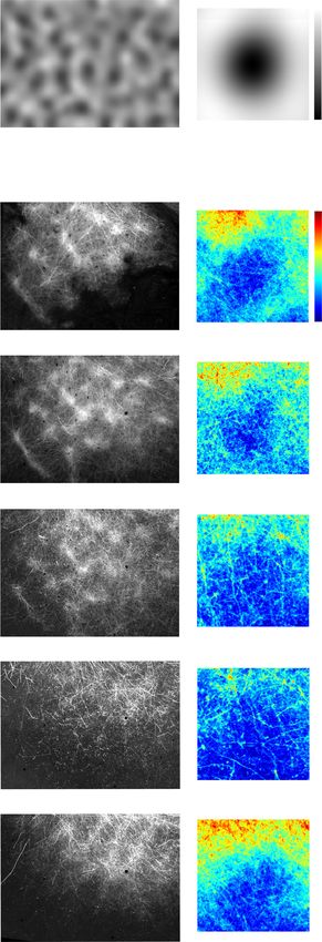
ARTICLE                                                                       NATURE COMMUNICATIONS | https://doi.org/10.1038/s41467-020-20505-5

                       a    OI                              ROI1                              ROI2                                 ROI2

                       V2
                                  TN        TN             TN            TN              TN                 TN                TN
                       V1

                                                                                   2mm
                       b    CO

                                    V2                                                                                   TN
                                                                                                TN         TN
                                    V1      TN             TN            TN

                       c    V2 injections

                            V2
                                         TN
                                                                                                                        TN

                             1 mm

                       d    V1 label

                             1 mm

Fig. 2 Segregated V2-to-V1 feedback pathways. Case MK374RHLat. a Functional maps recorded using optical imaging (OI). Left and middle: Orientation
difference map in two overlapping regions of interest (ROI1 and 2) encompassing V1 and V2, obtained by subtracting responses to achromatic gratings of
two orthogonal orientations (ROI1: 45–135°; ROI2: 90–0°). Solid yellow contour: V1/V2 border based on the orientation map. Dashed yellow contours
delineate the thin stripes (TN; regions of weak orientation responses). Right: SF difference map in ROI2, obtained by subtracting high-SF from low-SF
responses. Horizontal solid cyan contour: V1/V2 border based on the orientation map. Vertical cyan contours delineate TN (dashed) and thick (solid)
stripes, as regions having low-SF responsive domains (darker regions). b CO-stained tangential tissue sections 240 µm apart (left one is more superficial),
encompassing V1 and V2, revealing the stripes and the location of the two injection sites (ovals); the latter were determined by alignment of fluorescent
label to CO-stained sections (see Supplementary Fig. 1). Solid white contour: V1/V2 border based on CO staining. Dashed white contours delineate the
V2 stripes. Cyan and red box: locations of optically imaged ROI1 and 2, respectively, on the CO-stained sections. Scale bar in (a) valid for all panels in (a, b).
c Fluorescent micrographs of the AAV9-GFP and AAV9-tdT injection sites (shown at higher power in the inset below), outlined in green and red,
respectively, with superimposed outlines of TN stripes based on CO (white) and OI maps (yellow, orientation, cyan, SF). Note the good correspondence of
CO- and functionally-defined stripes. The injection outlines are shown overlaid to the V2 optical maps in (a) and CO sections in (b). d Micrograph of a
V1 section through L1B of V1 seen under GFP (LEFT) and tdT (MIDDLE) fluorescence, and with the two channels merged (RIGHT). Arrowheads point to
same blood vessels in all panels. GFP and tdT-labeled patches are interleaved. Label inside the white box is shown at higher power in (e), to demonstrate
lack of labeled somata, indicating anterograde viral expression. Results in (a–e) are representative of six independent injections centered in thin (n = 3) or
pale (n = 3) V2 stripes.

interblobs, across all layers of FB termination. Consistent with the              generate a heatmap of fluorescent signals for that layer (Supple-
laminar analysis shown above, the densest terminations were                       mentary Fig. 3d, Fig. 4b–f middle panels). The black circle on
located in L1/upper 2 and 5B-6, and sparser projections in L2/3                   each layer heatmap indicates the average blob diameter estimated
and 4B. To quantify the distribution of FB projections in the                     from the blobs used to compute the heatmap for that specific
blobs and interblobs of V1, for each layer we measured fluor-                      layer (as described in the “Methods” and in Supplementary
escent signal intensity within a square region of interest (ROI)                  Fig. 3a, b). In all layers, the highest fluorescence intensity lay
centered on each blob overlaying the FB termination zone, and                     outside the average blob border, indicating the densest FB ter-
encompassing the average blob and interblob diameter in the CO                    mination lay in the interblobs. The densest FB label, in this case,
map (see “Methods” and Supplementary Fig. 3a, c). Fluorescent                     was located in the upper right quadrant of the heatmaps, rather
signal intensity was, then, summed across all blob ROIs within a                  than uniformly filling the entire interblob region all around the
layer, and normalized to the maximum intensity value, to                          blob. Indeed the densest FB label was consistently located to one

4                  NATURE COMMUNICATIONS | (2021)12:228 | https://doi.org/10.1038/s41467-020-20505-5 | www.nature.com/naturecommunications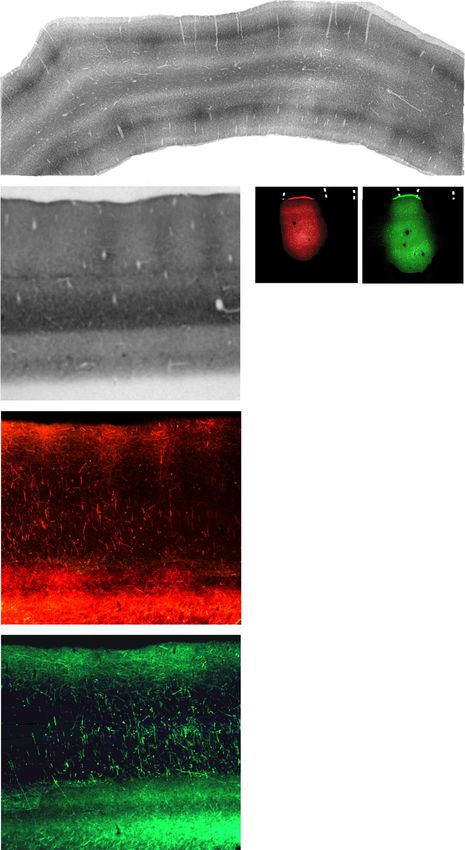
NATURE COMMUNICATIONS | https://doi.org/10.1038/s41467-020-20505-5                                                                        ARTICLE

                      a        OI
                                              TN
                                 TN

                                                                      1 mm
                      b    CO                                                  c   V2 injections
                                                                                           TN            TN

Fig. 3 Injection sites in V2 thick and thin stripes. Case MK356RH. Two AAV9-GFP injection sites, one confined to a V2 thick stripe, the other to a thin
stripe. a Orientation (45–135°; left) and SF (low-high; right) difference maps in V2. Dashed contours delineate regions having weak orientation responses
(yellow), and preferring low SFs (cyan), corresponding to thin stripes; solid white contour: V1/V2 border based on the orientation map.b Stack of aligned
and merged tangential V2 tissue sections stained for CO, revealing the stripe pattern. Red oval: imaged region from (a), determined based on the same
alignment procedure described for a different case in Supplementary Fig. 1. Dashed white contours outline the TN and thick stripes; solid black contour: V1/
V2 border based on the orientation map. c Micrographs of the two AAV9-GFP injection sites taken under fluorescent illumination and outlined, with
superimposed outlines of TN stripes based on CO (white) and OI maps (yellow, orientation, cyan, SF). Note the good correspondence between
functionally-defined and CO-defined stripes. The outlines of the injection sites (green ovals) indicate the location of the injection sites on CO sections (b)
and OI (a) maps. These injection sites in (a–c) are representative of six independent injections centered in thin (n = 3) or thick (n = 3) V2 stripes.

side of the blobs, in the termination zone, perhaps due to the                  FB label in V1 are shown in Fig. 2. A second example AAV9-GFP
small injection site being confined to few orientation domains in                injection site largely confined to a thin stripe (but slightly
the functional map of V2 (Fig. 3a), or due to the topographical                 encroaching into the adjacent pale-lateral stripe) is shown in
organization of FB connections, which precisely interconnect                    Fig. 3, and the FB axons in V1 labeled from this injection site are
matching retinotopic sites within the V1 and V2 CO compart-                     shown in Fig. 5 and Supplementary Fig. 2. Analysis of the dis-
ments. The heatmap for L4B showed much lower fluorescent                         tribution of FB labeled axons was performed as for the thick
label intensity compared to the other layers, but branching axons               stripe injection case described above. Qualitative observation
were clearly visible in this layer (Fig. 4e, left panel), and the               demonstrated patchy FB terminations, densest in V1 L1/upper 2
highest label intensity was still found within the interblobs                   and 5B-6, and sparser in L2/3, with little or no projections to L4B
(Fig. 4e, right panel).                                                         (Fig. 5b–f, left panels). Both qualitative and quantitative analyses
   From each layer heatmaps, we generated graphs of the                         revealed that the densest patches of labeled FB axons lay pre-
normalized fluorescence signal intensity as function of distance                 ferentially inside the blobs, although some sparser label also
from the center of the average blob (blue curves in right panels of             occurred in the interblobs, likely due to the injection site
Fig. 4b–f), as described in the “Methods” and Supplementary                     encroaching into the adjacent pale stripe (Fig. 5b–f, middle and
Fig. 3e. These curves were compared to similarly computed                       right panels). The heatmap for L4B showed no significant label
curves of CO signal intensity as function of distance from the                  (Fig. 5e, middle panel), with noisy background label in this layer
center of the average blob (black curves in right panels of                     being equally distributed across blobs and interblobs (Fig. 5e,
Fig. 4a–f, which were computed from the CO heatmap shown in                     right panel). Qualitative observations of L4B revealed only
the middle panel of Fig. 4a, as described in the “Methods” and in               punctate GFP label with little or no lateral axon branching,
Supplementary Fig. 3a, b, e). In all layers, the CO and fluorescent              suggesting this layer mainly contained unbranched axon trunks
signal curves showed similar trends, peaking at the largest                     traveling vertically (i.e., orthogonal to the plane of imaging)
distance from the blob center, indicating that the highest                      toward the superficial layers. This was in contrast to the branched
fluorescent signals coincided with the brightest regions in CO                   axonal label seen in this layer after both thick (Fig. 4e, left panel)
staining, i.e., the interblobs.                                                 and pale (Fig. 6e, left panel) stripe injections.
   The other two thick stripe injection cases showed similar results               The other two thin stripe injection cases showed similar results
to the case shown in Fig. 4, albeit, due to the smaller size of these           to the case shown in Fig. 5, but since these injection sites were
injections, the resulting V1 FB label was overall less dense and                more clearly confined to thin stripes, the terminal FB label
showed even greater specificity for the interblobs. Figure 7a                    showed even greater specificity for blobs. Figure 7b shows the thin
summarizes the thick stripe population data for all layers analyzed.            stripe population data for all layers analyzed.

V2 thin stripes project to V1 blobs. Three viral injections (2                  V2 pale stripes project to V1 interblobs. Three viral injections
AAV9-GFP, 1 AAV9-tdT, n = 3 animals) were confined to V2                         were confined to V2 pale stripes (1 AAV9-tdT in a pale-medial
thin stripes. One example AAV9-GFP injection site and resulting                 stripe and two AAV9-GFP in a pale-lateral stripe, n = 2 animals).

NATURE COMMUNICATIONS | (2021)12:228 | https://doi.org/10.1038/s41467-020-20505-5 | www.nature.com/naturecommunications                                   5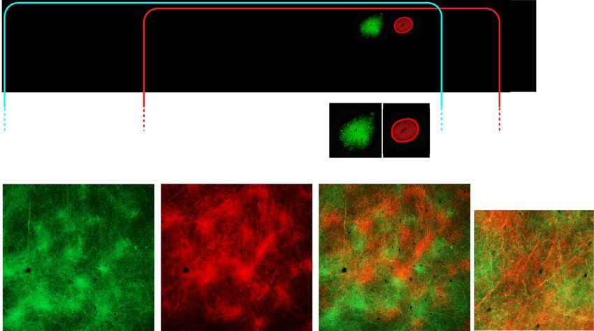
ARTICLE NATURE COMMUNICATIONS | https://doi.org/10.1038/s41467-020-20505-5
CO
1.0 1.0 CO
GFP
0.8 0.8
signal intensity
Normalized CO
0.6 0.6
0.4 0.4
0.2 0.2
0 0
0 1.0
1 mm Ictr Bctr Ictr Bctr Ictr
Normalized distance from Bctr
FB LABEL - Thick Stripes
1.0 L1A 1.0
0.8 0.8
signal intensity
0.6 0.6
Normalized
0.4 0.4
0.2 0.2
0 0
Ictr Bctr Ictr 0 1.0
L1B 1.0
0.8
0.6
0.4
0.2
0
0 1.0
L2/3 1.0
0.8
0.6
0.4
0.2
0
0 1.0
L4B 1.0
0.8
0.6
0.4
0.2
0
0 1.0
f L5/6 1.0
0.8
0.6
0.4
0.2
0
0 1.0
One example AAV9-tdT injection site confined to a pale-medial indicative of terminations within the layer. Both qualitative and
stripe is shown in Fig. 2a–c, and the FB axons in V1 labeled from quantitative analyses revealed that the densest patches of labeled
this injection site are shown in Figs. 2b–e and 6. FB axons from FB axons in all layers lay preferentially in the interblobs
this case also showed patchy FB terminations, densest in V1 L1/ (Fig. 6b–f, middle and right panels). Other pale-stripe injection
upper 2 and 5B-6, and sparser in L2/3 and L4B (Fig. 6b–f, left cases showed similar results. Figure 7c summarizes the pale-stripe
panels). FB terminals in L4B formed clear lateral branches population data for all layers analyzed.
6 NATURE COMMUNICATIONS | (2021)12:228 | https://doi.org/10.1038/s41467-020-20505-5 | www.nature.com/naturecommunications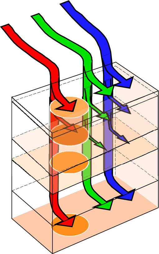
NATURE COMMUNICATIONS | https://doi.org/10.1038/s41467-020-20505-5                                                                             ARTICLE

Fig. 4 V2 thick stripes project to V1 interblobs. Case MK356RH. GFP-labeled FB axons in V1 after the thick stripe injection shown in Fig. 3. a Left: filtered
CO map from a section through V1 L2. Segmenting out the darkest 33% of pixels outlines the CO blobs (yellow). Scale bar valid also for (b–f, left). Middle:
heatmap of CO signal intensity, generated by measuring CO intensity within a 476 µm2 ROI centered around each blob, then summing all ROIs and
normalizing to maximum intensity (see “Methods” and Supplementary Fig. 3a, b). The average blob diameter (black circle) for this case was 284 µm. Right:
normalized CO signal intensity as a function of distance from the blob center (Bctr), computed from the CO heatmap, as described in the “Methods” and
Supplementary Fig. 3b, e. CO intensity is darkest in the Bctr and brightest in the interblob center (Ictr). The black CO-intensity curve is repeated on each plot
in (b–f, right) for comparison with the FB-label intensity curves. (b–f) Left: GFP-labeled FB axons in different V1 layers (indicated at the bottom left corner)
with superimposed the blob outlines (yellow) from (a, left). Dashed white lines in (b) outline the pial vessels. MIDDLE: heatmaps of the GFP-label intensity
for each layer, generated by measuring fluorescent signal intensity within an ROI centered on each blob overlaying the FB label in that layer, summing all
ROIs, and normalizing to maximum intensity. The size of the ROI in each layer is the average blob and interblob size within the FB termination zone in that
layer (see “Methods” and Supplementary Fig. 3a, c). Black circles: average blob diameter for that layer. Right: plots of normalized CO (black curves) and
GFP-fluorescence (blue curves) intensities as a function of distance from the Bctr, computed as described in the “Methods” and Supplementary Fig. 3b, d, e.
Here and in Figs. 5–7 right, the data were fitted with the following function: y = ax3 + bx2 + cx + d. In all layers, GFP-label intensity dominates in the
interblobs. Results in (a–f) are representative of three independent injections centered in thick stripes. Source data for right panels in (a–f) are provided as
a Source data file.

Population analysis. Figure 7 shows the summary data (see                         stripe types send densest projections to layers 1/upper 2 and 5B-6,
“Methods”) for the population of injections, grouped by stripe                    and sparser projections to lower layer 2 and layer 3. However,
type (n = 3 injections per stripe type). Like the individual                      only thick and pale, but not thin, stripes project to L4B (Fig. 8).
example cases, the population data shows that FB projections                         There has been a long-standing controversy regarding the
arising from V2 thick and pale stripes terminate preferentially in                clustering and specificity, or lack thereof, of FB connections to
the interblob regions of V1, across all layers of FB termination                  V1, mainly attributable to the technical limitations of the neu-
(Fig. 7a, c, respectively). In contrast, FB projections arising from              roanatomical tracers used in previous studies11. Conventional
V2 thin stripes terminate preferentially in the CO blobs (Fig. 7b).               tracers used to label FB axons were either transported ante-
Moreover, thick and pale, but not thin, stripes send FB projec-                   rogradely, but had poor sensitivity and resolution (e.g., tritiated
tions to L4B. Statistical comparison of the CO-compartment                        aminoacids, WGA-HRP, and first-generation adenoviral vectors),
location of densest FB label across stripe groups, for each V1                    or had good sensitivity, but were transported bidirectionally
layer, indicated no significant difference between pale and thick                  (CTB, BDA), thus labeling the axons of both FF- and FB-
stripes (L1A: p = 0.33, n = 20 for pale, n = 17 for thick; L1B: p =               projecting neurons. Studies using the first group of tracers
0.38, n = 28 for pale, n = 15 for thick; L2/3: p = 0.99, n = 15 for               injected in areas V2 or MT concluded that FB connections to V1
pale, n = 21 for thick; L4B: p = 0.6, n = 18 for pale, n = 12 for                 are diffuse, i.e., they make non-clustered terminations in their
thick; L5/6: p = 0.98, n = 26 for pale, n = 18 for thick;                         target areas, which are non-specific with respect to the CO
Kruskal–Wallis test with Bonferroni correction; n represents the                  compartments or functional domains of V128–30. Curiously,
number of bins within which fluorescent intensity was measured,                    however, one such study28 showed at least one example of patchy
over three independent injection cases for all comparisons, as                    FB axon terminations in layer 1 of macaque V1, but the authors
described in the “Methods”). In contrast, the CO-compartment                      did not comment on the modularity of FB connections. Studies
location of FB projections to V1 differed significantly between                    using injections of bidirectional tracers into V225,27 or V311,
thick and thin stripes, as well as between pale and thin stripes,                 instead, provided evidence for clustered11,25,27 and functionally
and this was the case for all layers of FB termination (p < 0.001 for             specific11,27 FB projections to V1. Due to the bidirectional
all comparisons and all layers but L4B for which p = 0.008 for the                transport of the tracers used in the latter studies, however, it was
thick versus thin comparison), except for L4B for the thin versus                 unclear whether the axon clustering reflected the termination
pale-stripe comparison which did not reach statistical significance                patterns of FB axons or of the axonal collaterals of the reciprocal
(p = 0.053), likely due to the low sample size (Kruskal–Wallis test               FF projection neurons, known to form patchy connections21,22,31.
with Bonferroni correction; the number of intensity bins exam-                    For the same reason, it had remained unclear whether FB pro-
ined over three independent injections for all thick vs. thin and                 jections to V1 terminate only in L1 and 6 (which do not send, or
pale vs. thin comparisons: L1A thick = 17, thin = 27, pale = 20;                  only send very sparse FF projections to extrastriate areas), or also
L1B thick = 15, thin = 19, pale = 28; L2/3 thick = 21, thin = 20,                 terminate in layers that send FF projections to higher cortical
pale = 15; L4B thick = 12, thin = 11, pale = 18; L5/6 thick = 18,                 areas (such as L2/3 and 4B). In a few studies, FB axons were
thin = 20, pale = 26). Moreover, when all layers data were pooled                 labeled by bulk injections of PHA-L or BDA in V2 or MT, and
together for each stripe group (see “Methods”), V2 thick and pale                 reconstructed through serial sections32–34. While these studies
stripes showed no significant difference in the V1 CO-                             were not affected by ambiguity in the interpretation of the origin
compartment location of their projections (p = 0.801), while                      of axonal label, they, however, provided a limited sample of
thick versus thin, and thin versus pale stripes were significantly                 partially reconstructed FB axons.
different from each other (p < 0.001 for all comparisons,                            To overcome the limitations of previous anatomical studies, in
Kruskal–Wallis test with Bonferroni correction, thick n = 83 bins,                this study we have taken advantage of recent advances in neu-
thin n = 97, pale n = 96).                                                        roanatomical labeling methods based on the use of viral vectors to
                                                                                  deliver genes for fluorescent proteins35. Specifically, we have used
Discussion                                                                        a mixture of AAV9-Cre and Cre-dependent-AAV9 to express
We have shown that FB projections arising from the different CO                   fluorescent proteins in V2 FB neurons projecting to V1 without
stripes of V2 do not diffusely and unspecifically contact all V1                   simultaneously labeling the axons of the reciprocal V1-to-V2 FF
regions within their termination zones, but rather form patchy                    projection neurons. Our results resolve existing controversies by
axon terminations which largely segregate in the CO compart-                      demonstrating unequivocally that FB connections from V2 to V1
ments of V1: thin stripes project predominantly to blobs, and                     form patchy terminations, in agreement with Angelucci et al.25
thick and pale stripes predominantly to interblobs. Moreover, all                 and Shmuel et al.27, and that the FB terminal patches are

NATURE COMMUNICATIONS | (2021)12:228 | https://doi.org/10.1038/s41467-020-20505-5 | www.nature.com/naturecommunications                                        7
ARTICLE NATURE COMMUNICATIONS | https://doi.org/10.1038/s41467-020-20505-5
CO
1.0 1.0 CO
GFP
0.8 0.8
signal intensity
Normalized CO
0.6 0.6
0.4 0.4
0.2 0.2
0 0
0 1.0
1 mm Ictr Bctr Ictr Bctr Ictr
Normalized distance from Bctr
FB LABEL - Thin Stripes
1.0
L1A 1.0
0.8 0.8
signal intensity
Normalized
0.6 0.6
0.4 0.4
0.2 0.2
0 0
Ictr Bctr Ictr 0 1.0
L1B 1.0
0.8
0.6
0.4
0.2
0
0 1.0
L2/3 1.0
0.8
0.6
0.4
0.2
0
0 1.0
L4B 1.0
0.8
0.6
0.4
0.2
0
0 1.0
L5/6 1.0
0.8
0.6
0.4
0.2
0
0 1.0
Fig. 5 V2 thin stripes project to V1 blobs. Case MK356RH. Same as in Fig. 4, but for GFP-labeled FB axons in V1 resulting from the AAV9-GFP injection
site in a V2 thin stripe shown in Fig. 3. In all layers, GFP-label intensity dominates inside blobs. Results in (a–f) are representative of three independent
injections centered in thin stripes. Source data for right panels in (a–f) are provided as a Source data file.
8 NATURE COMMUNICATIONS | (2021)12:228 | https://doi.org/10.1038/s41467-020-20505-5 | www.nature.com/naturecommunicationsNATURE COMMUNICATIONS | https://doi.org/10.1038/s41467-020-20505-5 ARTICLE
CO
1.0 1.0 CO
TDT
0.8 0.8
signal intensity
Normalized CO
0.6 0.6
0.4 0.4
0.2 0.2
0 0
0 1.0
1 mm
Ictr Bctr Ictr Bctr Ictr
Normalized distance from Bctr
FB LABEL - Pale Stripes
1.0 L1A 1.0
0.8 0.8
signal intensity
Normalized
0.6 0.6
0.4 0.4
0.2 0.2
0 0
Ictr Bctr Ictr 0 1.0
L1B 1.0
0.8
0.6
0.4
0.2
0
0 1.0
L2/3 1.0
0.8
0.6
0.4
0.2
0
0 1.0
L4B 1.0
0.8
0.6
0.4
0.2
0
0 1.0
L5/6 1.0
0.8
0.6
0.4
0.2
0
0 1.0
Fig. 6 V2 pale stripes project to V1 interblobs. Case MK374RHLat. Same as in Fig. 4, but for tdT-labeled FB axons in V1 resulting from the AAV9-tdT
injection site confined to a pale-medial stripe shown in Fig. 2a–c. In all layers, GFP-label intensity dominates in the interblobs. Results in (a–f) are
representative of three independent injections centered in pale stripes. Source data for right panels in (a–f) are provided as a Source data file.
NATURE COMMUNICATIONS | (2021)12:228 | https://doi.org/10.1038/s41467-020-20505-5 | www.nature.com/naturecommunications 9ARTICLE NATURE COMMUNICATIONS | https://doi.org/10.1038/s41467-020-20505-5
a Thick Stripes
L1A L1B L2/3 L4B L5/6
signal intensity
Normalized FB
Ictr Bctr Ictr
1.0 1.0 1.0 1.0 1.0
signal intensity
Normalized
0.8 0.8 0.8 0.8 0.8
0.6 0.6 0.6 0.6 0.6
0.4 0.4 0.4 0.4 0.4
0.2 0.2 0.2 0.2 0.2
0 0 0 0 0
0 1.0 0 1.0 0 1.0 0 1.0 0 1.0
Bctr Ictr CO signal
Normalized distance from Bctr FB signal
b Thin Stripes
1.0 1.0 1.0 1.0 1.0
0.8 0.8 0.8 0.8 0.8
0.6 0.6 0.6 0.6 0.6
0.4 0.4 0.4 0.4 0.4
0.2 0.2 0.2 0.2 0.2
0 0 0 0 0
0 1.0 0 1.0 0 1.0 0 1.0 0 1.0
c Pale Stripes
1.0
0.8
0.6
0.4
0.2
0
1.0 1.0 1.0 1.0 1.0
0.8 0.8 0.8 0.8 0.8
0.6 0.6 0.6 0.6 0.6
0.4 0.4 0.4 0.4 0.4
0.2 0.2 0.2 0.2 0.2
0 0 0 0 0
0 1.0 0 1.0 0 1.0 0 1.0 0 1.0
Fig. 7 Population analysis. Mean heatmaps of fluorescent signal intensity (top panels), and plots of fluorescent and CO signal intensities (bottom panels)
for the population of FB projections arising from a V2 thick stripes (n = 3), b thin stripes (n = 3), and c pale stripes (n = 3). For details of how the
population means were computed see “Methods”. Error bars in the fluorescent signal intensity plots are s.e.m. Statistical analysis of differences between
stripe types are reported in the “Results”. Conventions are as in Fig. 4. Source data for bottom panels in (a–c) are provided as a Source data file.
10 NATURE COMMUNICATIONS | (2021)12:228 | https://doi.org/10.1038/s41467-020-20505-5 | www.nature.com/naturecommunicationsNATURE COMMUNICATIONS | https://doi.org/10.1038/s41467-020-20505-5 ARTICLE
contact the same V1 cells, therefore integrating information
across these two parallel streams. However, current studies from
our laboratory, using rabies virus-mediated monosynaptic input
tracing to label direct inputs to V2-projecting neurons in V1,
suggest that FB projections from thick and pale stripes contact
predominantly distinct V1 projection neurons38.
Segregation of V1-to-V2 FF pathways within CO compart-
ments likely reflects specialized function, because CO compart-
ments in V1 and V2 show specialized neuronal responses
properties and functional maps. Specifically, the blob-thin-stripe
pathway is thought to process surface properties (color and
brightness), the interblob-pale-stripe pathway object contours
and form, and the interblob-thick stripe pathway object motion
and depth31,39–50. Our finding of segregated FB projections
within these same CO compartments, therefore, suggests that
V2 FB connections to V1 do not integrate information across
parallel functional streams, and thus across stimulus attributes,
but rather modulate V1 responses to the specific stimulus attri-
butes that are processed within their functional stream, an
organization that may support, for example, feature-selective
attention51,52, or the feature specificity of extraclassical receptive
field effects7,53,54.
Our finding of segregated V2-to-V1 FB pathways is consistent
Fig. 8 Parallel V2-to-V1 feedback pathways. Our proposed model of the
with previous results of stream-specific organization of cortico-
FB pathways from V2 to V1, based on the present study. The arrow
geniculate pathways in macaque55,56, suggesting this FB organi-
thickness indicates the relative density of projections to the different V1
zation may exist at multiple levels of the visual pathway. Our
layers (L4A is omitted). For all stripe types, layers 1/upper 2 and 5/6
results are also consistent with results in mouse visual cortex,
receive the densest FB projections, while lower L2 and L3 receive sparser
demonstrating segregation of functional FB channels from L5 of
projections from V2. Both thick (blue arrows) and pale (green arrows)
higher visual areas AL (anterolateral) and PM (posteromedial) to
stripes, but not thin (red arrows) stripes send FB projections to V1 L4B. FB
V157, which also matches the functional segregation of the reci-
projections from thin stripes predominantly target the V1 CO blob columns,
procal FF pathways from V1 to AL and PM58. Modular FB axon
while FB projections from thick and pale stripes predominantly target the V1
terminations have also been demonstrated anatomically in L1 of
interblob columns.
mouse V1, where FB axons from areas AL and PM form inter-
leaved terminal patches59. The FB patches from AL and PM, in
predominantly CO-compartment specific, in agreement with turn align with M2 muscarinic acetylcholine receptor-rich and
Shmuel et al.27. These results are also consistent with previous poor patches, respectively, which correspond to V1 regions spe-
demonstrations of patchy and CO-compartment-specific FB cialized for the processing of distinct spatio-temporal
connections from area V3 to V1 in macaque11. In particular, we features59,60. Interestingly, M2-positive patches are also found
demonstrate that in macaque monkey, FB connections arising in macaque V1 L1 where they are in register with the CO-poor
from the different CO stripes of V2 form parallel channels that interblobs60. Together with our results, these studies support the
mimic the reciprocal parallel pathways from V1 to V2 in this notion of functionally specialized parallel FB pathways.
species21. We also show that, with the exception of L1, the layers Our results of segregated FB pathways are consistent with
that give rise to FF connections to V2 (2/3, 4A, 4B, 5/6) receive predictive coding theories of FB function. According to these
reciprocal FB inputs. This suggests that V2 FB axons may make theories, the brain generates an internal model of the world, based
direct contacts with V1 neurons sending FF inputs to V2, a on sensory data and prior experience, which is refined by
hypothesis that we have recently confirmed using rabies virus- incoming sensory data. The latter is compared to the predicted
mediated monosynaptic input tracing to label monosynaptic sensory data, and the prediction error ascends up the cortical
inputs to V2-projecting neurons in V136. However, while L4B has hierarchy and refines the higher levels’ model5,61,62. Predictive
been shown to send at least some sparse inputs to thin and pale- coding models postulate the existence of different neuronal
medial stripes23,24,37, we only observed significant FB inputs to populations encoding expectations and prediction errors,
L4B from thick and pale, but not thin, stripes. It is possible that respectively, at each level of the cortical hierarchy. In these
our method of analysis failed to capture very sparsely labeled FB models, inter-areal FB connections carry the predictions, while FF
axons in L4B arising from thin stripes. Moreover, our low sample connections carry the error in those predictions12,13. In terms of
of injections into pale-medial stripes (n = 1) did not allow us to the architecture of hierarchical predictive coding schemes, one
assess potential quantitative differences in the FB projections to key attribute is the functional segregation of conditionally inde-
L4B from the two pale-stripe types, as has been previously pendent expectations, so that descending predictions are limited
demonstrated for the L4B to pale-stripe FF projections23. In this to prediction errors reporting a particular stimulus attribute, but
study, we have not analyzed L4A for potential FB terminations, as not prediction errors reporting opposite or different attributes.
this very thin layer is difficult to study in tangential sections, and For example, predictions about the orientation of a visual edge
in pia-to-white matter sections FB projections to L4A appeared to should not project to prediction errors units encoding visual
be, at best, very sparse. motion, because knowing the orientation of an edge does not,
Although here we are proposing the existence of at least three statistically, tell us anything about its motion. This suggests that
segregated FB pathways from V2 to V1, our study shows that FB direct descending predictions will be largely specific for stimulus
projections from thick and pale stripes both terminate in the attributes (e.g., contours vs. motion), which is consistent with our
interblobs, allowing for the possibility that these projections finding of FB-specific channels.
NATURE COMMUNICATIONS | (2021)12:228 | https://doi.org/10.1038/s41467-020-20505-5 | www.nature.com/naturecommunications 11ARTICLE NATURE COMMUNICATIONS | https://doi.org/10.1038/s41467-020-20505-5
While our results strongly support the existence of functionally speed. The pipette was left in place for an additional 5–10 min before being
specialized parallel FB pathways, it is noteworthy that our method retracted. These injection parameters yielded injection sites 1.3–1.8 mm in dia-
meter encompassing all cortical layers. For the cases used to investigate the dis-
of analysis was designed to extract the densest FB terminations in tribution of FB terminals relative to the V1 CO compartments, we used a similar
V1. However, lighter FB axonal label was visible in the regions procedure, but we injected smaller volumes in order to keep the injection site
between the densest labeled terminal patches. Therefore, we confined to a V2 stripe: 15–30 nl were injected at 1.2 mm depth, and an additional
cannot exclude that a smaller population of FB axons shows a 15–30 nl at 0.5–0.6 mm depth. Resulting injection sites ranged in diameter between
different terminal pattern, such as projections to all CO com- 0.56 and 0.95 mm and encompassed all V2 layers. One case used for the CO-
compartment analysis (MK356; Fig. 3) received a single injection of 105 nl in a thin
partments of V1 or projections to the opposite channel. This stripe and one injection of 75 nl in a thick stripe, both at a cortical depth of 1 mm.
population of FB axons may serve to integrate information across The resulting injection sites measured 1.26 and 0.65 mm in diameter, respectively,
streams, or to carry FB information about the same stimulus and encompassed all layers.
feature to neurons in different V1 CO compartments representing Each animal received 2–5 injections in dorsal area V2 of one hemisphere.
Within the same hemisphere either vectors expressing different fluorophores (GFP
that feature, for example orientation in the blobs and interblobs. or tdT) were injected, or injections of the same vector were spaced at least 10 mm
Similarly, FB from multiple stripes could affect the same neurons apart, to ensure no overlap of the resulting labeled fields in V1. In one case
within the same stimulus feature, for example both thick and pale (MK356), instead, two injections of the GFP-expressing vector were made in a
stripes have orientation maps, and FB to V1 from these stripes thick and a thin stripe within the same V2 stripe cycle (Fig. 3), which resulted in
two labeled fields in V1 that slightly overlapped (see Supplementary Fig. 2). In this
may be combined on the same V1 cells on the basis of orientation case, we excluded from analysis the region of label overlap.
preference.
Optical Imaging. Acquisition of intrinsic signals was performed using the Imager
Methods 3001 and VDAQ software (Optical Imaging Ltd, Israel) under red light illumina-
Experimental design. AAV9 vectors carrying the gene for either GFP or tdT were tion (630 nm). To identify the V2 stripes, we imaged V2 during presentation of
injected into specific V2 stripes, which in 3 animals were identified in vivo by gratings varying in orientation and SF. Orientation maps were obtained by pre-
intrinsic signal optical imaging. In two animals, instead, injections were made senting for 4 s full-field, high contrast (100%), pseudorandomized, achromatic
blindly with respect to stripe type. The V1 laminar and CO-compartment dis- drifting square-wave gratings of eight different orientations at 1.0–2.0 cycles/° SF,
tribution of FB axons labeled by these viral injections was analyzed quantitatively. moving back and forth at 1.5 or 2 cycles/s in directions perpendicular to the grating
orientation. Responses to same orientations were averaged across trials, following
baseline correction, and difference images were obtained by subtracting the
Animals. Five adult (aged 2–5 yrs old) cynomolgus macaque monkeys (Macaca
responses to two orthogonally oriented pairs (e.g., Figs. 2a, 3a). Imaging for SF (e.g.,
fasciculari; 4 females, 1 male) were used in this study. All procedures involving
Figs. 2a and 3a) was performed by presenting high contrast achromatic drifting
animals were approved by the Institutional animal Care and Use Committees of the
square-wave gratings of 6 different SFs (0.25, 0.5, 1, 1.5, 2, 3 cycles/°) alternating
University of Utah and conformed to the guidelines set forth by the USDA
through 8 different orientations every 500 ms, and drifting at 2 cycles/s. To create
and NIH.
SF difference maps, baseline-corrected responses to high SF (3 cycles/°) were
subtracted from baseline-corrected responses to low SF (0.25 cycles/°). Baseline
Surgical procedures. Animals were pre-anesthetized with ketamine (10–20 mg/kg, correction for both the orientation and SF maps was performed in three different
i.m.), intubated with an endotracheal tube, placed in a stereotaxic apparatus, and ways and the approach that provided the best maps was selected for analysis: (1)
artificially ventilated. Anesthesia was maintained with isofluorane (0.5–2.5%) in the baseline (pre-stimulus) was subtracted from the single condition response (i.e.,
100% oxygen, and end-tidal CO2, blood oxygenation level, electrocardiogram, and the images recorded during stimulation of one stimulus orientation or one SF); (2)
body temperature were monitored continuously. The scalp was incised, a cra- the single condition response was divided by the baseline; (3) the single condition
niotomy was made to expose the lunate sulcus and about 5 mm of cortex posterior response was divided by the “cocktail blank” (i.e., the average of responses to all
to it (encompassing V2 and a small portion of V1). In two animals (MK359, 4 oriented stimuli or all SF stimuli)63,64. Thick stripes were identified as the middle of
injections, and MK365, 3 injections) small durotomies were made just caudal to the regions having an orientation-preference map and domains responsive to low SFs;
posterior edge of the lunate sulcus, over V2, and viral vectors were injected into V2. pale stripes as regions having an orientation-preference map neighboring a region
In the reminder of cases (3 animals, total of 12 injections), optical imaging was with weak or no systematic orientation maps; and thin stripes as regions containing
used to identify the V2 stripes prior to the injections. In the latter cases, a large domains responsive to low SF, having weak or no systematic orientation maps
craniotomy and durotomy (15–20 mm mediolaterally, 6–8 mm anteroposteriorly) (Figs. 2a, 3a). In each case, reference images of the surface vasculature were taken
were performed to expose V2 and parts of V1, a clear sterile silicone artificial dura under green light (546 nm) illumination, and used in vivo as reference to position
was placed on the cortex, and the craniotomy was filled with a sterile 3% agar pipettes for viral vector injections, as well as postmortem to align the functionally
solution and sealed with a glass coverslip glued to the skull with Glutures (Abbott identified V2 stripes to the histological sections containing the injection sites and
Laboratories, Lake Bluff, IL). On completion of surgery, isoflurane was turned off sections labeled for CO to reveal the stripes (e.g., Figs. 2c, 3c, and Supplementary
and anesthesia was maintained with sufentanil citrate (5–10 µg/kg/h, i.v.). The Fig. 1).
pupils were dilated with a short-acting topical mydriatic agent (tropicamide), the
corneas protected with gas-permeable contact lenses, the eyes refracted, and optical
imaging was started. Once the V2 stripes were functionally identified (1–3 h of Histology. Areas V1 and V2 were dissected away from the rest of the visual cortex.
imaging, see below), the glass coverslip, agar, and artificial dura were removed and The block was postfixed for 1–2 h, sunk in 30% sucrose for cryoprotection, and
the viral vectors were injected in specific V2 stripe types, using surface blood vessels frozen-sectioned at 40 µm. For the cases used to investigate the distribution of FB
as guidance. On completion of the injections, new artificial dura was placed on the terminals across V1 layers (the cases in Fig. 1; n = 4), the block was cut perpen-
cortex, the craniotomy was filled with Gelfoam and sealed with sterile parafilm and dicularly to the layers and parallel to the V1–V2 border. This sectioning plane
dental cement, the skin was sutured and the animal was recovered from anesthesia. allows to easily identify layers, as well as the sequence of V2 stripes, which run
Animals survived 3–4 weeks post-injections, and underwent a terminal 3–5 day perpendicular to the border. For the reminder of the cases (n = 9), which were used
optical imaging experiment to obtain additional functional maps. At the conclu- for the analysis of FB terminals relative to the V1 CO compartments, instead, the
sions of this experiment the animal was sacrificed with Beuthanasia (0.22 ml/kg, block was postfixed between glass slides for 1–2 h to slightly flatten the cortex in
i.v.) and perfused transcardially with saline for 2–3 min, followed by 4% paraf- the optically imaged area, cryoprotected, and frozen-sectioned tangentially, parallel
ormaldehyde in 0.1 M phosphate buffer for 20 min. One animal was perfused with to the plane of the imaging camera. Sections were wet-mounted and imaged for
2% paraformaldehyde for 6 min and the brain postfixed overnight. fluorescent GFP and tdT-labeled cell bodies in V2 (the injection sites) and FB
axons in V1, using either Zeiss Axioskop 2 or Axio Imager Z2 microscopes (×10
magnification; software: Zen -blue edition-, Carl Zeiss Microscopy GmbH). After
Injections of viral vectors. A total of 19 viral vector injections were made in 5 digitizing the label, in most cases, the same sections were reacted for CO to reveal
macaque monkeys. We excluded from analysis 6 injections, which either did not the cortical laminae and V1 and V2 compartments, and then re-imaged under
produce detectable label in V1 (n = 2), or were located in an unidentifiable stripe bright field illumination (×1.25–5 magnification). In three cases, instead, the
(n = 4). The viral vectors consisted of a 1:1 mixture of AAV9.CaMKIIa.4.Cre.SV40 location of labeled axons for 2–3 sections was determined by alignment to
and either AAV9.CAG.Flex.eGFP.WPRE.bGH or AAV9.CAG.Flex.tdTomato. immediately adjacent CO-stained sections, rather than from the same section
WPRE.bGH (Penn Vector Core, University of Pennsylvania, PA), which were imaged for fluorescent label. In four cases, 1–2 sections were further immunor-
mixed and loaded in the same glass micropipette (tip diameter 35–45 µm), and eacted to enhance the GFP signal strength, and then imaged a third time using both
pressure injected using a picospritzer. For the injection cases used to investigate the bright field and fluorescent channels to maintain a perfect alignment between the
distribution of FB terminals across V1 layers (Fig. 1; n = 4), we slowly injected CO and label images. GFP immunohistochemistry was performed by incubating
(6–15 nl per min) 105–150 nl of the viral mixture at a cortical depth of 1.2 mm sections overnight at 4 °C in a chicken anti-GFP primary antibody (1:2000; RRID:
from the pial surface. After a 5 min pause, the pipette was retracted to a depth of AB_10000240), followed by incubation in Alexa Fluor 488 Donkey Anti-Chicken
0.5 mm, and an additional 105–150 nl of the viral mixture was injected at the same IgG secondary antibody (1:200; RRID:AB_2340375).
12 NATURE COMMUNICATIONS | (2021)12:228 | https://doi.org/10.1038/s41467-020-20505-5 | www.nature.com/naturecommunicationsYou can also read