Learning to Run challenge: Synthesizing physiologically accurate motion using deep reinforcement learning
←
→
Page content transcription
If your browser does not render page correctly, please read the page content below
Learning to Run challenge: Synthesizing physiologically
                                         accurate motion using deep reinforcement learning

                                         Łukasz Kidziński, Sharada P. Mohanty∗ , Carmichael Ong∗ , Jennifer L. Hicks, Sean F. Carroll, Sergey
                                         Levine, Marcel Salathé, Scott L. Delp
arXiv:1804.00198v1 [cs.AI] 31 Mar 2018

                                         Abstract Synthesizing physiologically-accurate human movement in a variety of conditions can help prac-
                                         titioners plan surgeries, design experiments, or prototype assistive devices in simulated environments, reduc-
                                         ing time and costs and improving treatment outcomes. Because of the large and complex solution spaces of
                                         biomechanical models, current methods are constrained to specific movements and models, requiring careful
                                         design of a controller and hindering many possible applications.
                                         We sought to discover if modern optimization methods efficiently explore these complex spaces. To do this,
                                         we posed the problem as a competition in which participants were tasked with developing a controller to
                                         enable a physiologically-based human model to navigate a complex obstacle course as quickly as possi-
                                         ble, without using any experimental data. They were provided with a human musculoskeletal model and a
                                         physics-based simulation environment.
                                         In this paper, we discuss the design of the competition, technical difficulties, results, and analysis of the
                                         top controllers. The challenge proved that deep reinforcement learning techniques, despite their high com-
                                         putational cost, can be successfully employed as an optimization method for synthesizing physiologically
                                         feasible motion in high-dimensional biomechanical systems.

                                         1 Overview of the competition

                                         Human movement results from the intricate coordination of muscles, tendons, joints, and other physiolog-
                                         ical elements. While children learn to walk, run, climb, and jump in their first years of life and most of us
                                         can navigate complex environments—like a crowded street or moving subway—without considerable active
                                         attention, developing controllers that can efficiently and robustly synthesize realistic human motions in a va-
                                         riety of environments remains a grand challenge for biomechanists, neuroscientists, and computer scientists.
                                         Current controllers are confined to a small set of pre-specified movements or driven by torques, rather than
                                         the complex muscle actuators found in humans (see Section 3.1).
                                             In this competition, participants were tasked with developing a controller to enable a physiologically-
                                         based human model to navigate a complex obstacle course as quickly as possible. Participants were provided
                                         with a human musculoskeletal model and a physics-based simulation environment where they could synthe-

                                          ∗   These authors contributed equally to this work

                                                                                                                                                      1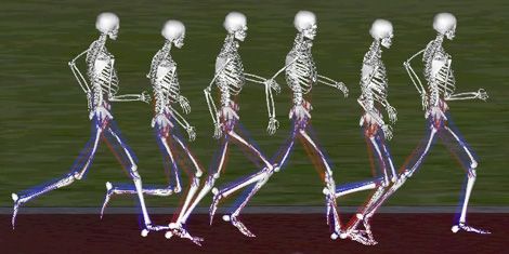
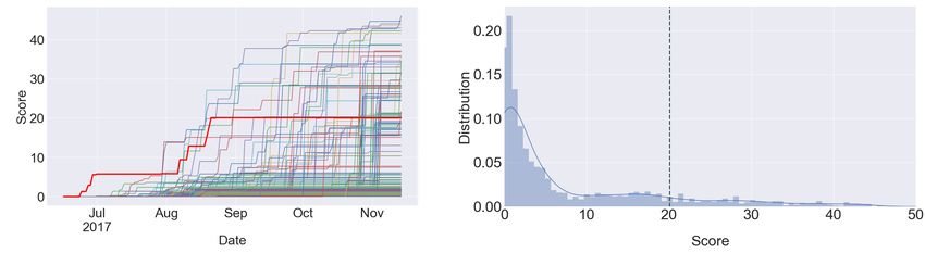
2                                                                               Authors Suppressed Due to Excessive Length

Fig. 1 Musculoskeletal simulation of human running in Stanford’s OpenSim software. OpenSim was used to simulate the
muscoloskeletal lower-body system used in the competition, and the competitors were tasked with learning controllers that
could actuate the muscles in the presence of realistic delays to achieve rapid running gaits. Image courtesy of Samuel Hamner.

size physically and physiologically accurate motion (Figure 1). Obstacles were divided into two groups:
external and internal. External obstacles consisted of soft balls fixed to the ground to create uneven terrain,
and internal obstacles included introducing weakness in the psoas muscle, a key muscle for swinging the
leg forward during running. Controllers submitted by the participants were scored based on the distance the
agents equipped with these controllers traveled through the obstacle course in a set amount of time. To simu-
late the fact that humans typically move in a manner that minimizes the risk of joint injury, controllers were
penalized for excessive use of ligament forces. We provided competitors with a set of training environments
to help build robust controllers; competitors’ scores were based on a final, unknown environment that used
more external obstacles (10 balls instead of 3) in an unexpected configuration (see Section 3.2).
   The competition was designed for participants to use reinforcement learning methods to create their
controllers; however, participants were allowed to use other optimization frameworks. As the benchmark,
we used state-of-the art reinforcement learning techniques: Trust Region Policy Optimization (TRPO) [17]
and Deep Deterministic Policy Gradients (DDPG) [15]. We included implementations of these reinforcement
learning models in the “Getting Started” tutorial provided to competitors.
   This competition fused biomechanics, computer science, and neuroscience to explore a grand challenge
in human movement and motor control. The entire competition was built on free and open source software.
Participants were required to tackle three major challenges in reinforcement learning: large dimensionality
of the action space, delayed actuation, and robustness to variability of the environments. Controllers that
can synthesize the movement of realistic human models can help optimize human performance (e.g., fine-
tune technique for high jump or design a prosthetic to break paralympic records) and plan surgery and
treatment for individuals with movement disorders (see Section 3.1). In Section 5, we analyze accuracy of
the top results from a biomechanical standpoint and discuss implications of the results and propose future
directions. For a description of solutions from top participants please refer to [13, 14].
   To the best of our knowledge, this was the largest reinforcement learning competition in terms of the num-
ber of participants and the most complex in terms of environment, to date. In Section 4 we share our insights
from the process of designing the challenge and our solutions to problems encountered while administering
the challenge.
Learning to Run challenge: Synthesizing physiologically accurate motion using deep reinforcement learning     3

2 Prior work

We identify two groups of prior challenges related to this proposal. The first set includes challenges held
within the biomechanics community, including the Dynamic Walking Challenge2 (exploring mechanics of
a very simple 2D walker) and the Grand Challenge Competition to Predict In Vivo Knee Loads3 (validation
of musculoskeletal model estimates of muscle and joint contact forces in the knee). In the Dynamic Walk-
ing Challenge, the model used was highly simplified to represent the minimimum viable model to achieve
bipedal gait without muscles. In the Grand Challenge, the focus was to predict knee loads given a prescribed
motion rather than to generate novel motions.
    The second class of prior challenges has been held in the reinforcement learning community. In the field
of reinforcement learning, competitions have periodically been organized around standardized benchmark
tasks4 . These tasks are typically designed to drive advancements in algorithm efficiency, exploration, and
scalability. Many of the formal competitions, however, have focused on relatively smaller tasks, such as sim-
ulated helicopter control [8], where the state and action dimensionality are low. More recently, vision-based
reinforcement learning tasks, such as the Arcade Learning Environment (ALE) [4] have gained popularity.
Although ALE was never organized as a formal contest, the Atari games in ALE have frequently been used
as benchmark tasks in evaluating reinforcement algorithms with high-dimensional observations. However,
these tasks do not test an algorithm’s ability to learn to coordinate complex and realistic movements, as would
be required for realistic running. The OpenAI gym benchmark tasks [5] include a set of continuous control
benchmarks based on the MuJoCo physics engine [23], and while these tasks do include bipedal running, the
corresponding physical models use simple torque-driven frictionless joints, and successful policies for these
benchmarks typically exhibit substantial visual artifacts and non-naturalistic gaits5 . Furthermore, these tasks
do not include many of the important phenomena involved in controlling musculoskeletal systems, such as
delays.
    There were three key features differentiating the “Learning to Run” challenge from other reinforcement
learning competitions. First, in our competition, participants were tasked with building a robust controller for
an unknown environment with external obstacles (balls fixed in the ground) and internal obstacles (reduced
muscle strength), rather than a predefined course. Models experienced all available types of obstacles in the
training environments, but competitors did not know how these obstacles would be positioned in the final test
obstacle course. This novel aspect of our challenge forced participants to build more robust and generalizable
solutions than for static environments such as those provided by OpenAI. Second, the dimensionality and
complexity of the action space were much larger than in most popular reinforcement learning problems.
It is comparable to the most complex MuJoCo physics OpenAI gym task Humanoid-V1 [5] which had
17 torque actuators, compared to 18 actuators in this challenge. In contrast to many robotics competitions,
the task in this challenge was to actuate muscles, which included delayed actuation and other physiological
complexities, instead of controlling torques. This increased the complexity of the relationship between the
control signal and torque generated. Furthermore, compared to torque actuators, more muscles are needed
to fully actuate a model. Third, the cost of one iteration is larger, since precise simulations of muscles are
computationally expensive. This constraint forces participants to build algorithms using fewer evaluations
of the environment.

2   http://simtk-confluence.stanford.edu:8080/pages/viewpage.action?pageId=5113821
3   https://simtk.org/projects/kneeloads
4   see, e.g., http://www.rl-competition.org/
5   see, e.g., https://youtu.be/hx_bgoTF7bs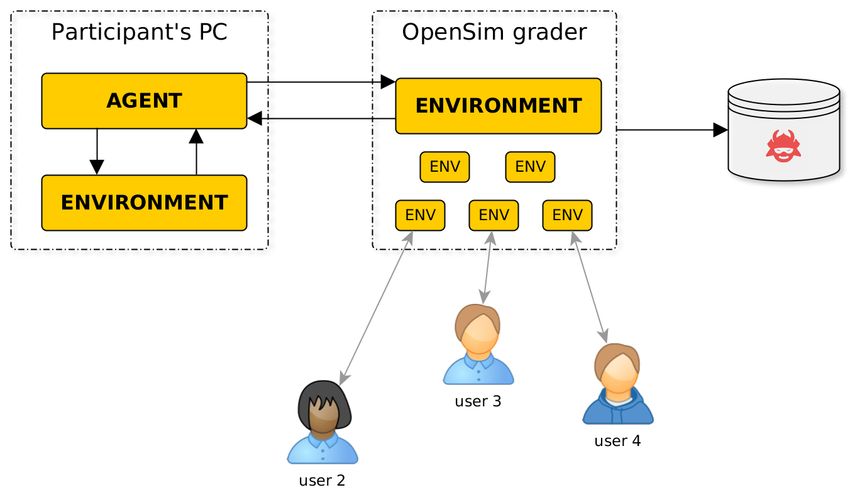
4                                                                      Authors Suppressed Due to Excessive Length

3 Competition description

3.1 Background

Understanding motor control is a grand challenge in biomechanics and neuroscience. One of the greatest
hurdles is the complexity of the neuromuscular control system. Muscles are complex actuators whose forces
are dependent on their length, velocity, and activation level, and these forces are then transmitted to the
bones through a compliant tendon. Coordinating these musculotendon actuators to generate a robust motion
is further complicated by delays in the biological system, including sensor delays, control signal delays,
and muscle-tendon dynamics. Existing techniques allow us to estimate muscle activity from experimental
data [22], but solutions from these methods are insufficient to generate and predict new motions in a novel
environment.
    Recent advances in reinforcement learning, biomechanics, and neuroscience can help us solve this grand
challenge. The biomechanics community has used single shooting methods to synthesize simulations of
human movement driven by biologically inspired actuators. Early work directly solved for individual muscle
excitations for a gait cycle of walking [3] and for a maximum height jump [2]. Recent work has focused on
using controllers based on human reflexes to generate simulations of walking on level ground [10]. This
framework has been extended to synthesize simulations of other gait patterns such as running [24], loaded
and inclined walking [9], and turning and obstacle avoidance [20]. Although these controllers were based
on physiological reflexes, they needed substantial input from domain experts. Furthermore, use of these
controllers has been limited to cyclic motions, such as walking and running, over static terrain.
    Modern reinforcement learning techniques have been used recently to train more general controllers for
locomotion. These techniques have the advantage that, compared to the gait controllers previously described,
less user input is needed to hand tune the controllers, and they are more flexible to learning additional, novel
tasks. For example, reinforcement learning has been used to train controllers for locomotion of complicated
humanoid models [15, 17]. Although these methods found solutions without domain specific knowledge,
the resulting motions were not realistic. One possible reason for the lack of human-like motion is that these
models did not use biologically accurate actuators.
    Thus while designing the “Learning to Run” challenge, we conjectured that reinforcement learning meth-
ods would yield more realistic results with biologically accurate models and actuators. OpenSim is an open-
source software environment which implements computational biomechanical models and allows muscle-
driven simulations of these models [7]. It is a flexible platform that can be easily incorporated into an opti-
mization routine using reinforcement learning.

3.2 OpenSim simulator

OpenSim is an open-source project that provides tools to model complex musculoskeletal systems in or-
der to gain a better understanding of how movement is coordinated. OpenSim uses another open-source
project, Simbody, as a dependency to perform the physics simulation. Users can employ either inverse meth-
ods, which estimate the forces needed to produce a given motion from data, or forward methods, which
synthesize a motion from a set of controls. In this competition, we used OpenSim to 1) model the human
musculoskeletal system and generate the corresponding equations of motion and 2) synthesize motions by
integrating the equations of motion over time.
Learning to Run challenge: Synthesizing physiologically accurate motion using deep reinforcement learning 5
The human musculoskeletal model was based on a previous model [6] and was simplified to decrease
complexity, similarly to previous work [16]. The model was composed of 7 bodies. The pelvis, torso, and
head were represented by a single body. Each leg had 3 bodies: an upper leg, a lower leg, and a foot. The
model contained 9 degrees of freedom (dof): 3-dof between the pelvis and ground (i.e., two translation and
one rotation), 1-dof hip joints, 1-dof knee joints, and 1-dof ankle joints.
The model included 18 musculotendon actuators [21], with 9 on each leg,
to represent the major lower limb muscle groups that drive walking (Figure 2).
For each leg, these included the biarticular hamstrings, short head of the biceps
femoris, gluteus maximus, iliopsoas, rectus femoris, vasti, gastrocnemius, soleus,
and tibialis anterior. The force in these actuators mimicked biological muscle as
the force depends on the length (l), velocity (v), and activation (a) level (i.e., the
control signal to a muscle that is actively generating force, which can range be-
tween 0% and 100% activated) of the muscle. Biological muscle can produce force
either actively, via a neural signal to the muscle to produce force, or passively, by
being stretched past a certain length. The following equation shows how the to-
tal force was calculated, due to both active and passive force, in the each muscle
(Fmuscle ),
Fmuscle = Fmax−iso (a factive (l) fvelocity (v) + f passive (l)),
where Fmax−iso is the maximum isometric force of a muscle (i.e., a stronger
muscle will have a larger value), factive and f passive are functions relating the active
and passive force in a muscle to its current length, and fvelocity is a function that
scales the force a muscle produces as a function of its current velocity (e.g., a
muscle can generate more force when lengthening than shortening). For a sense of
scale, in this model, values of Fmax−iso ranged between 557 N and 9594 N. Force
is transferred between the muscle and bone by tendons. Tendons are compliant
structures that generate force when stretched beyond a certain length. Given the
physical constraints between the tendon and muscle, a force equilibrium must be
satisfied between them, governed by the relationship,
Ftendon = Fmuscle cos(α),
Fig. 2 Musculoskeletal
where α is the pennation angle (i.e., the angle between the direction of the model in OpenSim used in
tendon and the muscle fibers). this competition. Red/pur-
Additionally, arbitrary amounts of force cannot be generated instantaneously ple curves indicate muscles,
due to various electrical, chemical, and mechanical delays in the biological sys- while blue balls attached to
feet model contact.
tem between an incoming electrical control signal and force generation. This was
modeled using a first-order dynamic model between excitation (i.e., the neural
signal as it reaches the muscle) and activation [21].
The model also had components that represent ligaments and ground contact. Ligaments are biological
structures that produce force when they are stretched past a certain length, protecting against excessively
large joint angles. Ligaments were modeled at the hip, knee, and ankle joints as rotational springs with
increasing stiffness as joint angle increases. These springs only engaged at larger flexion and extension
angles. Ground contact was modeled using the Hunt-Crossley model [12], a compliant contact model. Two
contact spheres were located at the heel and toes of each foot and generate forces depending on the depth6 Authors Suppressed Due to Excessive Length
and velocity of these spheres penetrating other contact geometry, including the ground, represented as a
half-plane, and other obstacles, represented as other contact spheres.
3.3 Tasks and application scenarios
In this competition, OpenSim and the model described in Section 3.2 served as a black-box simulator of
human movement. Competitors passed in excitations to each muscle, and OpenSim calculated and returned
the state, which contained information about joint angles, joint velocities, body positions, body velocities,
and distance to and size of the next obstacle. This occurred every 10 milliseconds during the simulation for
10 seconds (i.e., a total of 1000 decision time points).
At every iteration the agent receives the current observed state vector s ∈ R41 consisting of the following:
• Rotations and angular velocities of the pelvis, hip, knee and ankle joints,
• Positions and velocities of the pelvis, center of mass, head, torso, toes, and talus,
• Distance to the next obstacle (or 100 if it doesn’t exist),
• Radius and vertical location of the next obstacle.
Obstacles were small soft balls fixed to the ground. While it was possible to partly penetrate the ball, after
stepping into the ball the repelling force was proportional to the volume of intersection of penetrating body
and the ball. The first three balls were each positioned at a distance that was uniformly distributed between 1
and 5. Then, each subsequent obstacle was positioned at u meters after the last one, where u was uniformly
distributed between 2 and 4. Each ball was fixed at v meters vertically from the ground level, where v was
uniformly distributed between -0.25 and 0.25. Finally, the radius of each ball was 0.05 + v, where v was
drawn from an exponential distribution with a mean of 0.05.
Based on the observation vector or internal states, current strength and distance to obstacles, participants’
controllers were required to output a vector of current muscle excitations. These excitations were integrated
over time to generate muscle activations (via a model of muscle’s activation dynamics), which in turn gener-
ated movement (as a function of muscle moment arms and other muscle properties like strength and current
length and lengthening velocity). Participants were evaluated by the distance they covered in a fixed amount
of time. At every iteration the agent was expected to return a vector v ∈ [0, 1]18 of muscle excitations for the
18 muscles in the model.
Simulation environments were parametrized by: difficulty, seed and max_obstacles. Diffi-
culty corresponded to the number and density of obstacles. The seed was a number which uniquely identi-
fies pseudo-random generation of the obstacle positions in the environment and participants could use it in
training to obtain a robust controller. The seed ranges between 0 and 263 − 1. Both seed and difficulty
of the final test environment were unknown to participants. Such a setup allowed us to give access to in-
finitely many training environments, as well as choose the final difficulty reactively, depending on users’
performance leading up to the final competition round.
The controller modeled by participants was approximating functions of the human motor control sys-
tem. It collected signals from physiological sensors and generated signals to excite muscles. Our objective
was to construct the environment in such a way that its solutions could potentially help biomechanics and
neuroscience researchers to better understand the mechanisms underlying human locomotion.Learning to Run challenge: Synthesizing physiologically accurate motion using deep reinforcement learning 7
3.4 Baselines and code available
Before running the NIPS competition, we organized a preliminary contest, with similar rules, to better un-
derstand feasibility of the deep reinforcement learning methods for the given task. We identified that existing
deep learning techniques can be efficiently applied to the locomotion tasks with neuromusculoskeletal sys-
tems. Based on this experience, for the NIPS challenge, we used TRPO and DDPG as a baseline and we
included implementation of a simple agent in the materials provided to the participants.
One of the objectives of the challenge was to bring together researchers from biomechanics, neu-
roscience and machine learning. We believe that this can only be achieved when entering the compe-
tition and building the most basic controller is seamless and takes seconds. To this end, we wrapped
the sophisticated and complex OpenSim into a basic python environment with only two commands:
reset(difficulty=0, seed=None) and step(activations). The environment is freely avail-
able on GitHub6 and can be installed with 3 command lines on Windows, MacOS and Linux, using the
Anaconda platform7 . For more details regarding installation, refer to the Appendix.
3.5 Metrics
Submissions were evaluated automatically. Participants, after building the controller locally on their com-
puters, were asked to interact with a remote environment. The objective of the challenge was to navigate
through the scene with obstacles to cover as much distance as possible in fixed time. This objective
was measured in meters from the origin on the X-axis the pelvis traveled during the simulation. To promote
realistic solutions that avoid joint injury, we also introduced a penalty to the reward function for overusing
ligaments.
We defined the objective function as
Z Tp
reward(T ) = X(T ) − λ L(t)dt,
0
where X(T ) is the position of the pelvis at time T , L(t) is the sum of squared forces generated by ligaments
at time t and λ = 10−7 is a scaling factor. The value of λ was set very low due to an initial mistake in the
system and it turns the impact of ligament forces smaller than we initially designed. The simulation was
terminated either when the time reached T = 10s (equivalent to 1000 simulation steps), or when the agent
fell, which was defined as when the pelvis fell below 0.65m.
In order to fairly compare the participants’ controllers, the random seeds, determining muscle weakness
and parameters of obstacles, were fixed for all the participants during grading.
6 https://github.com/stanfordnmbl/osim-rl
7 https://anaconda.org/8 Authors Suppressed Due to Excessive Length
4 Organizational aspects
4.1 Protocol
Participants were asked to register on the crowdAI.org8 platform and download the “Getting Started” tutorial.
The guide led participants through installation and examples of training baseline models (TRPO and DDPG).
After training the model, participants connected to the grader and interacted with the remote environment,
using a submission script that we provided (Figure 4). The remote environment iteratively sent the current
observation and awaited response—the action of the participant in a given state. After that, the result was
sent to the crowdAI.org platform and was listed on the leaderboard (as illustrated in Figure 3). Moreover, an
animation corresponding to the best submission of a given user was displayed beside the score.
By interacting with the remote environment, participants could potentially explore it and tune their algo-
rithms for the test environment. In order to prevent this exploration and overfitting, participants were allowed
to send only five solutions per day. Moreover, the final score was calculated on a separate test environment
to which users can submit only 3 solutions in total.
At the beginning of the challenge we did not know, how many participants to expect, or if the difficulty
would be too low or too high. This motivated us to introduce two rounds:
1. The Open Stage was open for everyone and players were ranked by their result on the test environment.
Every participant was allowed to submit 1 solution per day.
2. The Play-off Stage was open only for the competitors who earned at least 15 points in the Open Stage.
Participants were allowed to submit only 3 solutions. Solutions were evaluated on a test environment
different than the one in Open Stage.
The Play-off Stage was open for one week after the Open Stage was finished. This setting allowed us to
adjust the rules of the Play-off before it starts, while learning more about the problem and dynamics of the
competition in the course of the Open Stage.
We anticipated that the main source of cheating for locomotion tasks could be tracking of real or engi-
neered data. To avoid this problem, we designed the competition such that competitors were scored on an
unknown environment with obstacles, which means that a controller solely based on tracking is very unlikely
to be successful.
To prevent overfitting as well as cheating, participants did not have access to the final test environment.
Moreover, since participants were only interacting with a remote environment (as presented in Figure 4),
they were not allowed to change parameters of the environment, such as gravity or obstacles. In fact, they
were constrained to send only action vectors in v ∈ [0, 1]18 to the grader.
4.2 Execution
In the Open Stage, participants interacted with the environment through a lightweight HTTP API included
in the osim-rl package. From a technical standpoint, in order to interact with a remote environment, they
only needed to change the class from the local environment to HTTP API environment. The grader, on the
remote host, was responsible for the life-cycle management of the environments. The cumulative rewards for
each submission were added to the crowdAI leaderboard, along with visualization of the actual simulations.
8 http://crowdai.org/Learning to Run challenge: Synthesizing physiologically accurate motion using deep reinforcement learning 9 Fig. 3 The leaderboard from the first round (Open Stage) of the “Learning to Run” challenge on the crowdAI.org platform. We conjecture that animated simulations contributed to engagement of participants. To judge submissions, 3 seeds for simulation environments were randomly chosen beforehand and were used to grade all submissions during this stage. In the Play-off stage, participants packaged their agents into self-contained Docker containers. The con- tainers would then interact with the grader using a lightweight redis API, simulating the process from the Open Stage. The grading infrastructure had a corresponding Docker image for the actual grading container. Grading a single submission involved instantiating the participant submitted Docker container, instantiat- ing the internal grading container, mapping the relevant ports of the grading container and the submitted container, wrapping up both the containers in a separate isolated network, and then finally executing the pre-agreed grading script inside the participant submitted container.
10                                                                                Authors Suppressed Due to Excessive Length

Fig. 4 Schematic overview of the model training and submission process in the competition. Participants trained their agents on
local machines, where they could run the environment freely. Once the agent was trained, they connected to the grader and, in
an iterative process, they received the current state of the environment to which they responded with an action. After successful
iteration until the end condition (10 seconds of a simulation or a fall of the agent), the final result was stored in the crowdAI
database. Multiple users could connect to the grader simultaneously—each one to a separate environment.

4.3 Problems and Solutions

The major issues we encountered concerned the computational cost of simulations, over-fitting, and stochas-
ticity of the results, i.e. high dependence of the random seed. Our solutions to each of these challenges are
described below.
    The Learning to Run environment was significantly slower than many visually similar environments
such as the humanoid robot Mujoco-based simulations in OpenAI Gym9 . This difference was due to the
complex ground reaction model, muscle dynamics, and precision of simulation in OpenSim. Some of the
participants modified the accuracy of OpenSim engine to trade off precision for execution speed10 ; even with
these changes, the OpenSim-based Learning to Run environment continued to be expensive in terms of the
actual simulation time. The computationally expensive nature of the problem required participants to find
sample-efficient alternatives.
    Another concern was the possibility of overfitting, since the random seed was fixed, and the number of
simulations required for a fair evaluation of performance of submitted models. These issues were especially
important in determining a clear winner during the Play-off stage. To address these issues, we based the
design of the Play-off stage on Docker containers, as described in 4.2.

9   https://github.com/stanfordnmbl/osim-rl/issues/78
10   https://github.com/ctmakro/stanford-osrl#the-simulation-is-too-slow
Learning to Run challenge: Synthesizing physiologically accurate motion using deep reinforcement learning 11
The design based on Docker containers has two main advantages for determining the top submissions.
First, we could run an arbitrary number of simulations until we got performance scores for the top agents
which were statistically significant. Given the observed variability of results in the Open Stage, we chose 10
simulations for the Play-off Stage and it proved to be sufficient for determining the winner. See Section 4.4
for details. Second, this setting prevents overfiting, since users do not have access to the test environment,
while it allows us to use exactly the same environment (i.e., the same random seed) for every submission.
The main disadvantage of this design is the increased difficulty of submitting results, since it requires
familiarity with the Docker ecosystem. For this reason, we decided to use this design only in the Play-off
stage. This could potentially discourage participation. However, we conjectured that top participants who
qualified to the Play-off stage will be willing to invest more time in preparing the submission, for the sake of
fair and more deterministic evaluation. All top 10 participants from the Open Stage submitted their solutions
to the Play-off stage.
4.4 Submissions
The competition was held between June 16th 2017 and November 13th 2017. It attracted 442 teams with
2154 submissions. The average number of submission was 4.37 per team, with scores ranging between
−0.81 and 45.97 in both stages combined. In Figure 5 we present the progression of submissions over time.
Fig. 5 Left: Progression of scores during the challenge. Each curve represents the maximum score of a single participant on
the leaderboard at any point in time. The bold red line represents the baseline submission. Right: The final distribution of the
scores for all the submitted solutions. The dotted gray line represents the score (20.083) of the baseline submission.
The design of the Play-off stage allowed us to vary the number of simulations used to determine the
winner. However, our initial choice of 10 trials turned out to be sufficiently large to clearly determine the top
places (Figure 6).
From the reports of top participants [14, 13], we observed that most of the teams (6 out of 9) used
DDPG as the basis for their final algorithm while others used Proximal Policy Optimization (PPO) [18].
Similarly, in a survey we conducted after the challenge, from ten respondents (with mean scores 17.4 and
standard deviation 14.1) five used DDPG, while two used PPO. This trend might be explained by the high
computational cost of the environment, requiring the use of data efficient algorithms.12 Authors Suppressed Due to Excessive Length
Fig. 6 Distribution of scores per simulation of the top 3 submitted entries in the Play-off Stage. In the final round of the
challenge we ran 10 simulations in order to reduce the impact of randomness on the results. As it can be seen in the plot,
the scores of top three participants were rather consistent between the simulations. This indicates that, despite stochasticity of
simulations, our protocol allowed to determine the winner with high degree of confidence.
5 Results
We conducted a post-hoc analysis of the submitted controllers by running the solutions on flat ground with
no muscle weakness (i.e., max_obstacles=0, difficulty=0). Only the last 5 seconds of each sim-
ulation were analyzed in order to focus on the cyclic phase of running. To compare simulation results with
experimental data, we segmented the simulation into individual gait cycles, which are periods of time be-
tween when a foot first strikes the ground until the same foot strikes the ground again. For each submission,
all gait cycles were averaged to generate a single representative gait cycle. We compared the simulations
to experimental data of individuals running at 4.00 m/s [11] as it is the closest speed to the highest scoring
submissions.
Figure 7 compares the simulated hip, knee, and ankle joint angle trajectories with experimental data,
separated by three bins of scores: 1) over 40, 2) between 30 and 40, and 3) between 25 and 40. These bins
represent solutions with the following rankings: 1) 1st through 5th, 2) 6th through 24th, and 3) 25th through
47th. Solutions in all of the score bins show some promising trends. For example, solutions in all three score
bins have joints that are extending, shown by decreasing angle values, through the first 40% of the gait cycle
indicating that the models are pushing off the ground at this phase. Joint angles begin flexing, shown by
increasing angle values during the last 60% of the gait cycle in order to lift the leg up and avoid tripping.
There were a few notable differences between the simulations and the running gait of humans. At the hip,
simulations have a greater range of motion than experimental data as solutions both flex and extend more
than is seen in human running. This could be due to the simple, planar model. At the knee, simulations had
an excessively flexed knee at initial contact of the foot (i.e., 0% of the gait cycle) and had a delayed timingLearning to Run challenge: Synthesizing physiologically accurate motion using deep reinforcement learning 13
Fig. 7 Simulated hip, knee, and ankle angle trajectories (black lines) compared to 20 experimental subjects running at 4.00
m/s (gray regions) [11]. Results are plotted from left to right with decreasing performance in three bins: scores over 40 (left),
between 30 and 40 (middle), and between 25 and 30 (right). Positive values indicate flexion, and negative values indicate
extension. 0% gait cycle indicates when the foot first strikes the ground.
of peak knee flexion compared to experimental data (i.e., around 80% of the gait cycle compared to 65% of
the gait cycle).
Future work can be done to improve the current results. Improving the fidelity of the model could yield
better results. For example, allowing the hip to adduct and abduct (i.e., swing toward and away from the
midline of the body) would allow the leg to clear the ground with less hip flexion and reduce the excessive hip
range of motion. Testing different reward functions may also improve results, such as adding terms related
to energy expenditure [24]. Finally, it is likely that the best solution still has not been found, and further
improvements in reinforcement learning methods would help to search the solution space more quickly,
efficiently and robustly.
6 Discussion
The impact of the challenge ranged across multiple domains. First, we stimulated new techniques in rein-
forcement learning. We also advanced and popularized an important class of reinforcement learning prob-
lems with a large set of output parameters (human muscles) and comparatively small dimensionality of14 Authors Suppressed Due to Excessive Length
the input (state of a dynamic system). Algorithms developed in the complex biomechanical environment
also generalize to other reinforcement learning settings with highly-dimensional decisions, such as robotics,
multivariate decision making (corporate decisions, drug quantities), stock exchange, etc.
This challenge also directly impacted the biomechanics and neuroscience communities. The control mod-
els trained could be extended to and validated in, for example, a clinical setting to help predict how a patient
will walk after surgery [1]. The controllers developed may also approximate human motor control and thus
deepen our understanding of human movement. Moreover, by the analogy to Alpha Go, where reinforcement
learning strategy outperforms humans [19] due to broader exploration of the solution space, in certain human
movements we may potentially find strategies more efficient in terms of energy or accuracy. Reinforcement
learning is also a powerful tool for identifying deficiencies and errant assumptions made when building
models, and so the challenge can improve on the current state-of-the-art for computational musculoskeletal
modeling.
Our environment was setup using an open-source physics engine - a potential alternative for commercial
closed-source MuJoCo, which is widely used in the reinforcement learning research community. Similarly,
crowdAI.org–the platform on which the challenge was hosted–is also an open-source alternative to Kaggle11 .
By leveraging the agile infrastructure of crowdAI.org and components from OpenAI reinforcement learning
environments12 , we were able to seamlessly integrate the reinforcement learning setting (which, to the date,
is not available in Kaggle).
This challenge was particularly relevant to the NIPS community as it brought together experts from both
neuroscience and computer science. It attracted 442 competitors with expertise in biomechanics, robotics,
deep learning, reinforcement learning, computational neuroscience, or a combination. Several features of
the competition ensured a large audience. Entries in the competition produced engaging (and sometimes
comical) visuals of a humanoid moving through a complex environment. Further, we supplied participants
with an environment that is easy to set-up and get started, without extensive knowledge of biomechanics.
7 Affiliations and acknowledgments
Łukasz Kidziński, Carmichael Ong, Jennifer Hicks and Scott Delp are affiliated with Department of Bio-
engineering, Stanford University. Sharada Prasanna Mohanty, Sean Francis and Marcel Salath are affiliated
with Ecole Polytechnique Federale de Lausanne. Sergey Levine is affiliated with University of California,
Berkeley.
The challenge was co-organized by the Mobilize Center, a National Institutes of Health Big Data to
Knowledge (BD2K) Center of Excellence supported through Grant U54EB020405. It was partially spon-
sored by NVIDIA, Amazon Web Services, and Toyota Research Institute.
References
1. Ackermann, M., Van den Bogert, A.J.: Optimality principles for model-based prediction of human gait. Journal of biome-
chanics 43(6), 1055–1060 (2010)
11 https://kaggle.com/
12 https://github.com/kidzik/osim-rl-graderLearning to Run challenge: Synthesizing physiologically accurate motion using deep reinforcement learning 15
2. Anderson, F.C., Pandy, M.G.: A dynamic optimization solution for vertical jumping in three dimensions. Computer meth-
ods in biomechanics and biomedical engineering 2(3), 201–231 (1999)
3. Anderson, F.C., Pandy, M.G.: Dynamic optimization of human walking. Journal of biomechanical engineering 123(5),
381–390 (2001)
4. Bellemare, M.G., Naddaf, Y., Veness, J., Bowling, M.: The arcade learning environment: An evaluation platform for general
agents. Journal of Artificial Intelligence Research 47, 253–279 (2013)
5. Brockman, G., Cheung, V., Pettersson, L., Schneider, J., Schulman, J., Tang, J., Zaremba, W.: Openai gym. arXiv preprint
arXiv:1606.01540 (2016)
6. Delp, S., Loan, J., Hoy, M., Zajac, F., Topp, E., Rosen, J.: An interactive graphics-based model of the lower extremity to
study orthopaedic surgical procedures. IEEE Transactions on Biomedical Engineering 37(8), 757–767 (1990)
7. Delp, S.L., Anderson, F.C., Arnold, A.S., Loan, P., Habib, A., John, C.T., Guendelman, E., Thelen, D.G.: Opensim: open-
source software to create and analyze dynamic simulations of movement. IEEE transactions on biomedical engineering
54(11), 1940–1950 (2007)
8. Dimitrakakis, C., Li, G., Tziortziotis, N.: The reinforcement learning competition 2014. AI Magazine 35(3), 61–65 (2014)
9. Dorn, T.W., Wang, J.M., Hicks, J.L., Delp, S.L.: Predictive simulation generates human adaptations during loaded and
inclined walking. PloS one 10(4), e0121,407 (2015)
10. Geyer, H., Herr, H.: A muscle-reflex model that encodes principles of legged mechanics produces human walking dynamics
and muscle activities. IEEE Transactions on neural systems and rehabilitation engineering 18(3), 263–273 (2010)
11. Hamner, S.R., Delp, S.L.: Muscle contributions to fore-aft and vertical body mass center accelerations over a range of
running speeds. Journal of Biomechanics 46(4), 780–787 (2013)
12. Hunt, K., Crossley, F.: Coefficient of restitution interpreted as damping in vibroimpact. Journal of Applied Mechanics
42(2), 440–445 (1975)
13. Jaśkowski, W., Lykkebø, O.R., Toklu, N.E., Trifterer, F., Buk, Z., Koutnı́k, J., Gomez, F.: Reinforcement Learning to Run...
Fast. In: S. Escalera, M. Weimer (eds.) NIPS 2017 Competition Book. Springer, Springer (2018)
14. Kidziński, Ł., Mohanty, S.P., Ong, C., Huang, Z., Zhou, S., Pechenko, A., Stelmaszczyk, A., Jarosik, P., Pavlov, M.,
Kolesnikov, S., Plis, S., Chen, Z., Zhang, Z., Chen, J., Shi, J., Zheng, Z., Yuan, C., Lin, Z., Michalewski, H., Mio, P.,
Osiski, B., andrew, M., Schilling, M., Ritter, H., Carroll, S., Hicks, J., Levine, S., Salath, M., Delp, S.: Learning to run
challenge solutions: Adapting reinforcement learning methods for neuromusculoskeletal environments. In: S. Escalera,
M. Weimer (eds.) NIPS 2017 Competition Book. Springer, Springer (2018)
15. Lillicrap, T.P., Hunt, J.J., Pritzel, A., Heess, N., Erez, T., Tassa, Y., Silver, D., Wierstra, D.: Continuous control with deep
reinforcement learning. arXiv preprint arXiv:1509.02971 (2015)
16. Ong, C.F., Geijtenbeek, T., Hicks, J.L., Delp, S.L.: Predictive simulations of human walking produce realistic cost of trans-
port at a range of speeds. In: Proceedings of the 16th International Symposium on Computer Simulation in Biomechanics,
pp. 19–20 (2017)
17. Schulman, J., Levine, S., Abbeel, P., Jordan, M.I., Moritz, P.: Trust region policy optimization. In: ICML, pp. 1889–1897
(2015)
18. Schulman, J., Wolski, F., Dhariwal, P., Radford, A., Klimov, O.: Proximal policy optimization algorithms. arXiv preprint
arXiv:1707.06347 (2017)
19. Silver, D., Schrittwieser, J., Simonyan, K., Antonoglou, I., Huang, A., Guez, A., Hubert, T., Baker, L., Lai, M., Bolton, A.,
et al.: Mastering the game of go without human knowledge. Nature 550(7676), 354 (2017)
20. Song, S., Geyer, H.: A neural circuitry that emphasizes spinal feedback generates diverse behaviours of human locomotion.
The Journal of physiology 593(16), 3493–3511 (2015)
21. Thelen, D.G.: Adjustment of muscle mechanics model parameters to simulate dynamic contractions in older adults. Journal
of Biomechanical Engineering 125(1), 70–77 (2003)
22. Thelen, D.G., Anderson, F.C., Delp, S.L.: Generating dynamic simulations of movement using computed muscle control.
Journal of Biomechanics 36(3), 321–328 (2003)
23. Todorov, E., Erez, T., Tassa, Y.: Mujoco: A physics engine for model-based control. In: Intelligent Robots and Systems
(IROS), 2012 IEEE/RSJ International Conference on, pp. 5026–5033. IEEE (2012)
24. Wang, J.M., Hamner, S.R., Delp, S.L., Koltun, V.: Optimizing locomotion controllers using biologically-based actuators
and objectives. ACM transactions on graphics 31(4) (2012)16 Authors Suppressed Due to Excessive Length
8 Appendix
8.1 Installation
We believe that the simplicity of use of the simulator (independently of the skills in computer science
and biomechanics) contributed significantly to the success of the challenge. The whole installation pro-
cess took around 1-5 minutes depending on the internet connection. To emphasize this simplicity let us
illustrate the installation process. Users were asked to install Anaconda (https://www.continuum.
io/downloads) and then to install our reinforcement learning environment by typing
conda create -n opensim-rl -c kidzik opensim git
source activate opensim-rl
pip install git+https://github.com/kidzik/osim-rl.git
Next, they were asked to start a python interpreter which allows interaction with the musculoskeletal model
and visualization of the skeleton (Figure 8) after running
from osim.env import GaitEnv
env = GaitEnv(visualize=True)
observation = env.reset()
for i in range(500):
observation, reward, done, info = env.step(env.action_space.sample())
Fig. 8 Visualization of the environment with random muscles activations after. This simulation is immediately visible to the
user after following simple installation steps as described in Appendix.You can also read