Within-Generation Polygenic Selection Shapes Fitness-Related Traits across Environments in Juvenile Sea Bream - MDPI
←
→
Page content transcription
If your browser does not render page correctly, please read the page content below
G C A T
T A C G
G C A T
           genes
Article
Within-Generation Polygenic Selection Shapes
Fitness-Related Traits across Environments in
Juvenile Sea Bream
Carine Rey 1,2 , Audrey Darnaude 3 , Franck Ferraton 3 , Bruno Guinand 1 , François Bonhomme 1 ,
Nicolas Bierne 1 and Pierre-Alexandre Gagnaire 1, *
 1   ISEM, Univ Montpellier, CNRS, EPHE, IRD, Montpellier, France; carine.rey@ens-lyon.fr (C.R.);
     bruno.guinand@umontpellier.fr (B.G.); francois.bonhomme@umontpellier.fr (F.B.);
     nicolas.bierne@umontpellier.fr (N.B.)
 2   Univ Lyon, ENS de Lyon, Univ Claude Bernard, CNRS UMR 5239, INSERM U1210, Laboratoire de Biologie
     et Modélisation de la Cellule, 15 parvis Descartes, F-69007 Lyon, France
 3   MARBEC, Univ Montpellier, CNRS, IRD, Ifremer, 34095 Montpellier, France;
     audrey.darnaude@umontpellier.fr (A.D.); franck.ferraton@umontpellier.fr (F.F.)
 *   Correspondence: pierre-alexandre.gagnaire@umontpellier.fr

 Received: 1 March 2020; Accepted: 4 April 2020; Published: 7 April 2020

 Abstract: Understanding the genetic underpinnings of fitness trade-offs across spatially variable
 environments remains a major challenge in evolutionary biology. In Mediterranean gilthead sea
 bream, first-year juveniles use various marine and brackish lagoon nursery habitats characterized
 by a trade-off between food availability and environmental disturbance. Phenotypic differences
 among juveniles foraging in different habitats rapidly appear after larval settlement, but the relative
 role of local selection and plasticity in phenotypic variation remains unclear. Here, we combine
 phenotypic and genetic data to address this question. We first report correlations of opposite signs
 between growth and condition depending on juvenile habitat type. Then, we use single nucleotide
 polymorphism (SNP) data obtained by Restriction Associated DNA (RAD) sequencing to search for
 allele frequency changes caused by a single generation of spatially varying selection between habitats.
 We found evidence for moderate selection operating at multiple loci showing subtle allele frequency
 shifts between groups of marine and brackish juveniles. We identified subsets of candidate outlier
 SNPs that, in interaction with habitat type, additively explain up to 3.8% of the variance in juvenile
 growth and 8.7% in juvenile condition; these SNPs also explained significant fraction of growth rate
 in an independent larval sample. Our results indicate that selective mortality across environments
 during early-life stages involves complex trade-offs between alternative growth strategies.

 Keywords: antagonistic pleiotropy; habitat association; fitness trade-off; juvenile growth; polygenic
 scores; RAD-sequencing; spatially varying selection

1. Introduction
      Understanding how species adapt to heterogeneous environments is a central objective in
evolutionary biology and ecology [1–4]. This basic question has important ramifications for our
understanding of diversification and extinction and therefore has gained practical importance for
predicting species resilience in the face of rapid global change [5,6]. Population genomic approaches
facilitate the identification and characterization of adaptive genetic variation in nature [7–10]. However,
deciphering the complex mechanisms underlying local adaptation remains a challenging issue
that needs to explicitly consider the links connecting genotype to phenotype and fitness across
environments [11].

Genes 2020, 11, 398; doi:10.3390/genes11040398                                  www.mdpi.com/journal/genes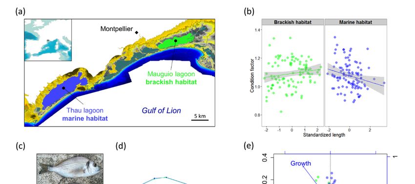
Genes 2020, 11, 398                                                                                   2 of 17

      The main obstacle to establishing such connections occurs when selection affects complex
quantitative traits that are themselves encoded by many genes [12,13]. In these situations, genome-wide
association (GWA) studies between complex traits and single nucleotide polymorphisms (SNPs) usually
lack the power to detect loci with small individual effects on phenotype [14,15]. Moreover, the small
allele frequency changes generated by polygenic selection represent a major challenge for ecological
genomics studies that search for single locus signatures of selection in molecular data [13,16].
      Polygenic selection may however generate heterogeneous patterns with both subtle and large allele
frequency changes [17–19], in particular when local selection occurs in an unpredictable, heterogeneous
environment [9]. Indeed, when dispersal occurs on a large scale compared to environmental variation,
genotypes are exposed to spatially varying selective pressures, which maintain polygenic variation
among individuals [20,21]. Under high gene flow conditions, the migration–selection balance tends to
favor intermediate and large effect loci that better resist gene swamping [3,22]. It is therefore likely
that, under such conditions, the outlier loci detected in genome scans for selection collectively explain
a significant (although incomplete) fraction of the genetic variance for fitness traits [19]. Unfortunately,
the joint contribution of candidate variants to phenotypic variation is rarely assessed in empirical
genome scan studies, although some studies have proved its interest for connecting genotype to
phenotype and fitness [23–25]. Here, we implement this approach in a high gene flow marine fish
species, to test whether phenotypic differentiation established within a single generation reflects
differential survival of genotypes at loci affecting traits, as opposed to pure phenotypic plasticity.
      Our model, the gilthead sea bream (Sparus aurata L.), is a seasonal migratory fish which uses
highly heterogeneous habitats throughout its life cycle. Adults reproduce at sea during winter and the
3–4-month-long larval duration ensures efficient mixing of drifting larvae before they recruit to coastal
juvenile habitats [26]. In the Gulf of Lion (northwestern Mediterranean), sea bream postlarvae settle in
various types of nursery habitats in March–April without evidence for habitat choice and probably
remain within the same habitat over the entire summer before returning to the open sea at the juvenile
stage in October–November when water temperatures drop [26,27]. Multielemental otolith fingerprints
have revealed that, in the Gulf of Lion, only 15% of the first-year juveniles stay in the nearshore
marine habitat, whereas the majority of juveniles use shallow brackish lagoons (47%) or deep marine
coastal lagoons (38%) for foraging [27,28]. Marine lagoons have a low food productivity compared to
brackish ones but offer much more stable conditions with regards to variations in physicochemical
parameters (e.g., oxygen, temperature, salinity) [29]. This trade-off between food availability and
environmental disturbance translates into phenotypic differences (including growth rate, condition
and shape) between juveniles foraging in different habitats, which rapidly appear a few months
after recruitment [26]. The genetic basis of these phenotypic differences and the possible role of
diversifying selection remain unclear, although genotype-by-environment interactions have been
detected at growth-related candidate genes [30,31].
      In this study, we specifically investigated the genotype–phenotype–fitness links across different
juvenile environments by combining population genomics and quantitative genetics approaches. To
this aim, we jointly analyzed phenotypic and genomic variation in a single cohort of wild sea bream,
including newly settled larvae and juveniles that foraged in contrasted (brackish vs. marine) lagoon
environments. We developed a test to detect allele frequency shifts caused by a single generation of
selection and evaluated the extent to which outlier loci additively contribute to survival probability in
each environment. Furthermore, we used polygenic scores to test whether spatially varying selection
affecting multiple loci partly explains the observed environment-dependent correlation between
growth and condition, and the larval growth rate. Our study illustrates how spatially varying selection
acting on complex traits involved in alternative growth strategies can help maintain variation at loci
affecting survival in different environments.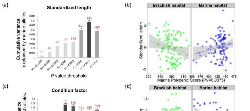
Genes 2020, 11, 398 3 of 17
2. Materials and Methods
2.1. Sampling
Genes 2020, 11, x FOR PEER REVIEW 3 of 17
Wild sea bream were sampled from two different nursery habitats of a single population in the
95 2. Materials and Methods
northern part of the Gulf of Lion, Southern France (Figure 1a). We collected three samples from the
same96year2.1. cohort (2013), consisting of (i) newly settled postlarvae (N = 44), (ii) young juveniles (0+)
Sampling
from97 the Mauguio Wild seabrackish
bream werelagoon
sampled = 106)
(Nfrom and (iii)nursery
two different young juveniles
habitats (0+)population
of a single from theinThau the marine
lagoon = 106), part
98 (N northern which represent
of the theSouthern
Gulf of Lion, main nursery habitats
France (Figure 1a). in
Wethe region.
collected threePostlarvae
samples from were
the collected
99 same year cohort (2013), consisting of (i) newly settled postlarvae (N
at the entrance of Thau lagoon in early spring, and juveniles were collected at different points in = 44), (ii) young juveniles (0+)
both100lagoonsfrom the Mauguio brackish lagoon (N = 106) and (iii) young juveniles (0+) from the Thau marine
during summer and fall of the same year (Table S1, see Supplementary for full details).
101 lagoon (N = 106), which represent the main nursery habitats in the region. Postlarvae were collected
Mauguio
102 and
at theThau lagoons
entrance of Thauare separated
lagoon by lessand
in early spring, than 30 km,
juveniles werea sufficiently small points
collected at different geographical
in both scale to
ensure103 that all individuals
lagoons during summer belong
and tofallthe same
of the samepanmictic
year (Tablepopulation, since genetic
S1, see Supplementary for fullhomogeneity
details). has
been104 Mauguio
observed and Thau
at much lagoons
larger are separated
spatial scales inby less than 30study
a previous km, a sufficiently
[30]. Thissmalldesign geographical
enabled scale
us to compare
105 diversity
genetic to ensure that all individuals belong to the same panmictic population, since genetic homogeneity
within the postlarval pool (i.e., before postsettlement selective mortality) to genetic
106 has been observed at much larger spatial scales in a previous study [30]. This design enabled us to
diversity
107 within
comparetwo groups
genetic of within
diversity youngthe juveniles
postlarvalthat
pool were grown
(i.e., before in ecologically
postsettlement selectivecontrasted
mortality) habitats
(i.e.,108
selected in different
to genetic diversityenvironments).
within two groups of The twojuveniles
young sampled thatbrackish
were grown and marine nurseries
in ecologically contrasted represent
109 ends
different habitats
of (i.e., selected in
a trade-off different food
between environments).
availabilityThe two
andsampled brackish and
environmental marine nurseries
disturbance that occur in
110 represent different ends of a trade-off between food availability and environmental disturbance that
the coastal waters of the Gulf of Lion [27]. The brackish habitat (Mauguio lagoon) has a high primary
111 occur in the coastal waters of the Gulf of Lion [27]. The brackish −1
habitat (Mauguio lagoon) has a high
production
112 (mean
primary annual (mean
production Chl aannual
concentration of 56.1ofµg
Chl a concentration 56.1Lµg L)−1and
) and provides suitable
provides suitable conditions for
conditions
rapid 113growth. However,
for rapid growth.itHowever,
also shows important
it also temporaltemporal
shows important variations of physicochemical
variations of physicochemical parameters
114
(temperature, parameters (temperature,
salinity, dissolvedsalinity,
oxygen) dissolved
due to oxygen) due to its
its shallow shallow
depth (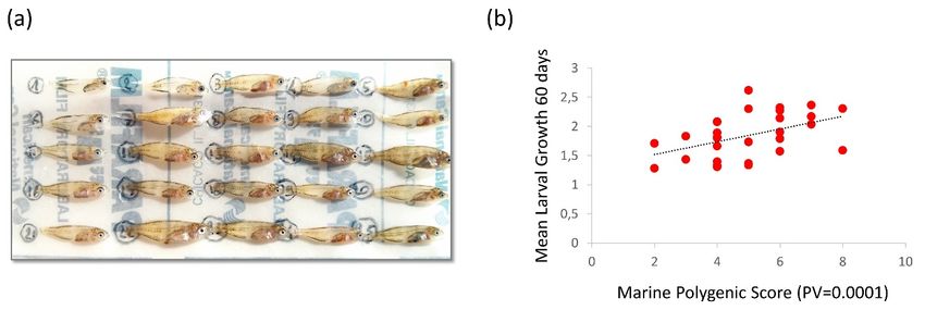
Genes 2020, 11, 398                                                                                4 of 17

2.2. Scoring of Phenotypes
     We collected two phenotypic traits, condition factor and growth, which are generally considered
as good indicators of fitness in fish [32]. Each juvenile was measured (total length in mm from head to
the end of caudal fin) and weighted (eviscerated weight in g). The relative condition factor (K) was
calculated as the ratio of its measured weight to the predicted weight obtained from the log–log linear
regression of weight against length based on all juvenile samples [33]. Total lengths were centered
to mean zero and normalized to unit variance within each habitat for each sampling date to avoid
scaling difficulties due to heterochronous sampling. We thus produced a standardized length index
capturing interindividual growth differences while controlling for a possible effect of sampling date on
total length. Linear correlations were tested between individual standardized length and condition
factor in each habitat. Since we found slopes of opposite signs, we specifically tested the interaction
between individual standardized length and habitat type (brackish vs. marine) for the condition factor
response using an analysis of covariance (ANCOVA) in R, which allows fitting different slopes and
intercepts in each habitat using lm(formula = Condition ~ Habitat × Std length).
     The predictive accuracy of the standardized index as a surrogate for individual somatic growth
rate was evaluated using otolith age reading in 40 juveniles. Twenty fish from each lagoon were
prepared following the protocol of [26] to obtain fish age and calculate somatic growth rate in mm
per day. Refined readings were also performed in those 40 juveniles to separately estimate the otolith
larval growth rate as the average daily width increment of otolith rings (in µm per day) during the first
60 days of larval life and the juvenile summer otolith growth rate as the average daily width increment
during June and July. In addition, 30 of the 44 larvae were submitted to refined otolith reading to
estimate individual otolith growth rate during the 60 first days of larval life.
     A picture of the left lateral side of 145 randomly selected juveniles was used to perform
morphometric measurements in tpsDig 2.17 [34]. Photographs were digitized with 22 anatomically
homologous landmarks covering the entire body. A generalized Procrustes analysis was performed
using the R package geomorph [35], and aligned Procrustes coordinates were used to estimate the mean
shape of juveniles in each nursery habitat. We then used the R package vegan [36] to estimate the
extent to which individual shape was influenced by experimental variables using the model Shape
~ Sampling date + Habitat + Std length + Condition. The significance of each factor was tested using
a redundancy analysis (RDA) marginal effects permutation test (1000 permutations). Finally, we
analyzed the influence of growth and condition on shape independently from temporal effects using a
partial RDA under the model Shape ~ Std length + Condition, removing the effect of Sampling date.

2.3. RAD Sequencing, Variant Calling and Individual Genotyping
     Genomic DNA was isolated from each of the 256 individuals (larvae and juveniles) using the
NucleoSpin Tissue Kit (Macherey-Nagel), standardized to 25 ng µL−1 and digested with the restriction
enzyme SbfI-HF. Eight Restriction Associated DNA (RAD) libraries were constructed by multiplexing 32
uniquely barcoded individuals per library, following a protocol adapted from previous studies [37,38].
Each library was then sequenced on a separate lane of an Illumina HiSeq2000 instrument with 101 bp
single-end reads.
     Illumina reads were demultiplexed and quality filtered using process_radtags in Stacks [39,40] and
subsequently trimmed to 86 bp (Figure S1). Cleaned individual reads were de novo assembled with
ustacks using a minimum read depth (−m) of 5 × per individual per allele and allowing at most three
mismatches (−M) between two alleles for a same locus. We used the ‘bounded error rate’ model with
a maximal error rate of 1% for SNP calling. These parameters were optimized in preliminary runs
using different individuals (Figure S2). A catalog of loci was then constructed with cstacks, allowing
at most three mismatches (–N) between alleles within loci. Each individual was finally matched
back to the catalog of loci using sstacks, and the program populations was used to export genotypes
using a minimum call rate of 70% in at least two of the three samples and a minor allele frequency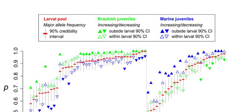
Genes 2020, 11, 398                                                                                 5 of 17

(maf) threshold of 1%. Individual genotypes were exported as biallelic SNPs as well as multiallelic
haplotypes defined by reads at the scale of single RAD-tags.
      The two polymorphism datasets (SNPs and haplotypes) were further filtered to include only loci
with no missing data in at least 90% of the individuals within each of the three samples (larvae, brackish
and marine juveniles). We then excluded markers showing significant deviation from Hardy–Weinberg
equilibrium within at least one sample using a P-value threshold of 10−3 in PLINK [41]. This filter
mainly aims at removing loci showing strong heterozygote excesses or deficiencies and should not
significantly interfere with our capacity to subsequently detect loci influenced by section. Indeed, even
strong spatially varying selection can be compatible with HWE proportions [42]. Finally, we used a
custom script to detect systematic bias in read counts in favor of a given allele across individuals. For
each locus, the allele with the lowest overall read count was identified to compute the ratio of lower to
higher allele read depth for each heterozygote. Loci showing significant deviation to the expected ratio
of 0.5 (one-sided t-test, P-value threshold of 0.05) were excluded from the datasets.

2.4. Genetic Homogeneity among Samples
    The overall genetic structure among all individuals was examined using a principal component
analysis (PCA) in the R package adegenet [43]. Genetic differentiation between larval and juvenile
samples and between brackish and marine juveniles was estimated using pairwise FST for each
polymorphism dataset (SNPs and haplotypes).

2.5. Test for Single-Generation Selection
      In order to detect within-generation allele frequency changes that are unlikely to occur by random
chance alone, we developed a statistical test based on a previous method that detects selective changes
occurring within a single generation [44]. Our approach takes into account two different sources of
allele frequency variance, one due to the finite size of the population, which influences the allele
frequency spectrum, and the other due to the finite sample size, which influences the level of uncertainty
in measuring the real allele frequencies from population samples. We considered a panmictic common
gene pool from which two samples of size N1 and N2 are drawn within the same generation, either
at two different times or in two different environments. For a given allele at a given biallelic locus,
the observed allele frequency difference between the two samples (∆p = p1 − p2 ) was compared
with the null distribution of ∆p expected from random sampling effects (i.e., due to finite sample size
effects). The mathematical details of the method are described as Supplementary Methods and Figures
(Figures S3 and S4).
      The power of the test was evaluated using simulations and compared to Fisher’s exact test, which
is classically used to test for genetic differentiation. We considered a finite panmictic population
(N = 10, 000) from which two samples of size N1 and N2 were drawn within the same generation.
Selection only occurred in sample 2 with genotypes’ fitness coefficients ωAA = 1 + s, ωAa = 1 and
ωaa = 1 − s. The value of ∆p was calculated after selective mortality, genetic drift and sampling effects,
using 100 simulations for each combination of initial allele frequency and selection coefficient value
(p, s). Power was measured as the proportion of tests rejecting the null hypothesis of ∆p = 0 at a 5%
significance level for each combination of p and s values (Figure S5).
      The test for detecting single-generation selection (SGS) was finally applied to the SNP dataset
to compare brackish (N = 105) versus marine (N = 102) juveniles, using 10,000 iterations to estimate
P-values.

2.6. Estimating the Survival Probability of Genotypes
     We used the subset of outlier loci detected with the SGS test (P-value threshold of 10−3 ) to perform
a PCA using all individuals. The distribution of larval genotypes in the plane defined by the first
two PC axes was used as a representation of the initial genetic composition within the larval pool
before postsettlement selection. This multilocus diversity was then compared to that observed in each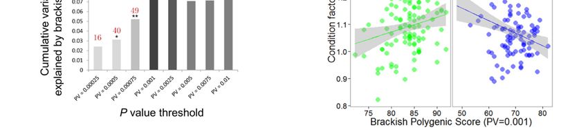
Genes 2020, 11, 398                                                                                  6 of 17

juvenile sample in order to estimate the relative enrichment or depletion of genotypes after selection
over the genotypic space. For each of the three samples, individual coordinates on the first two PCs
were used to perform two-dimensional kernel density estimation using the kde2D function in the R
package MASS. We then calculated the difference between juvenile and larval density estimates to
estimate a relative survival probability surface within each habitat. The genotype of each individual
was then projected on this surface to get individual survival probability scores in each habitat.

2.7. Genotype–Phenotype Links
     Genome-wide association (GWA) study was used to identify RAD markers linked with causative
variants underlying variation in standardized length and condition. Quantitative-trait association
analysis was performed using three different models in PLINK [41]: (i) a simple linear model capturing
the additive effect of each individual SNP on the phenotype y = β0 + β1 x + ε; (ii) a linear model
including juvenile environment as a covariate y = β0 + β1 x + β2 E + ε; and (iii) a linear model including
a genotype-by-environment interaction term y = β0 + β1 x + β2 E + β3 G × E + ε. We used the P-value
of the SNP term for the first two models (i.e., with or without adjustment for environmental effects) and
the interaction term P-value for the third model (i.e., the significance of the difference between the two
regression coefficients in each habitat). The genome-wide significance threshold was adjusted using
Bonferroni correction by taking within-RAD-tag linkage disequilibrium into account. Quantile–quantile
(Q–Q) plots and Manhattan plots were drawn using the R package qqman.
     In order to test whether selected genes collectively contribute to phenotypic variation in interaction
with the environment, we performed ANCOVA based on individual polygenic scores for both growth
using lm(formula = Std length ~ Habitat × Polygenic Score) and condition using lm(formula = Condition ~
Habitat × Polygenic Score). Individual polygenic scores were obtained by summing over all significant
SNPs the number of alleles that are favored in a given environment. We thus obtained a marine
polygenic score and a brackish polygenic score that measure the cumulative effects of alleles that
were inferred to be advantageous in the marine and brackish habitat, respectively. Because of the
low amount of missing genotypes per individual (3.7%), we did not correct for missing data in the
calculation of individual polygenic scores. Therefore, marine and brackish polygenic scores (that
sum to 2 times the number of loci in the absence of missing data) were computed separately for each
individual and separately tested in the ANCOVA. Individual polygenic scores were computed for
different sets of loci that were detected at different P-value cutoffs in the SGS test to determine the
nominal significance threshold maximizing the amount of total phenotypic variance explained by the
ANCOVA for each trait [19].
     The genotype-by-environment interaction for growth was then tested using the juvenile summer
otolith growth rate measured as the average daily width increment (in µm per day) during 60 days in
June–July. Although this strongly decreased the power of the tests due to data availability for otolith
growth rates in only 40 samples, it provided a better estimation of summer growth as compared to the
standardized length.
     Finally, we evaluated the genotype–phenotype relationships using an independent sample of
larvae that were not used for outlier SNP detection. Mean otolith growth rate from 30 larvae during
the 60 first days of larval life were used to test for association between larval growth and polygenic
scores using the linear model lm(formula= Larval growth ~ Polygenic Score).

3. Results

3.1. Phenotypic Variation
     The average condition factor did not differ significantly between brackish and marine juveniles
(marine K̂ = 0.996, brackish K̂ = 1.011, t-test P = 0.2). However, the ANCOVA model for the condition
response was significant (P = 0.014, R2 = 0.050, Figure 1b) and revealed significantly different regression
slopes of individual condition versus standardized length between habitats (P = 0.003). Condition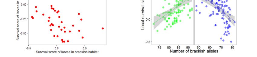
Genes 2020, 11, 398                                                                                 7 of 17

tended to be positively correlated with standardized length in the brackish habitat, but negatively
correlated in the marine habitat. Otolith daily increments and age readings in 40 juveniles confirmed
that the standardized length provides a good substitute measure for both individual somatic growth
rate (R2 = 0.77, Figure 1c) and otolith growth rate calculated from birth to sampling date (R2 = 0.40).
Therefore, standardized length was used as a measure of somatic growth in the remaining analyses,
since this phenotype was available for all juvenile fish, which was not the case for otolith readings. For
the larval sample, a particular effort was made to measure the daily width increment of otolith rings
during the first 60 days of larval life, which averaged to 1.84 ± 0.37 µm per day. This refined measure
of larval growth rate was obtained in 30 individuals to test for genotype–phenotype correlations in the
larval sample.
      Mean body shape differed significantly between habitats (Figure 1d), as revealed by the
permutation test for Procrustes distances between groups (P < 0.001). On average, brackish juveniles
displayed a larger body height between first dorsal spine and anterior pectoral-fin insertion compared
with marine juveniles. All factors had significant marginal effects in the RDA of body shape (P < 0.001).
The effect of standardized length and condition remained significant (P < 0.001) after controlling for
sampling date. The two axes of the partial RDA constrained by standardized length and condition
after removing the sampling date effect explained 7.8% of the total morphological variance, and partly
separated brackish and marine juveniles (Figure 1e). In the marine sample, the direction of maximum
variance among individuals coincided with RDA axis 2, highlighting a negative correlation between
standardized length and condition. In the brackish habitat, individual projections were preferentially
distributed along the vector indicating the main gradient of variation in standardized length.

3.2. Population Genetic Homogeneity
    A total of 34,679 SNPs (17,579 haplotype markers) were retained after filtering for genotype quality.
We detected no evidence of population structure from each of these two datasets (SNPs and haplotypes).
Genetic differentiation (FST ) was almost zero in all pairwise sample comparisons (Table S2). Genetic
homogeneity was also illustrated by the perfect overlap of all three samples in the PCA (Figure S6).

3.3. Genotype–Fitness Links
      The test to detect allele frequency shifts caused by single generation selection (SGS) outperformed
Fisher’s exact test for genetic differentiation in most simulations (Figure S5). Applying the SGS test
between brackish and marine juveniles detected 67 outliers at the nominal significance threshold of
10−3 (Figure 2). For most of these SNPs (86.6%), the major allele frequency observed in the larval
sample was intermediate to the values observed in juveniles from brackish and marine habitats, and for
71.6% of them at least one juvenile sample lay outside the 90% posterior credibility interval estimated
from the larval sample. Also, for the majority of these outliers (59.7%), the major allele increased in
frequency in the brackish habitat compared to the larval sample. For simplicity, we later refer to those
alleles as “brackish alleles”, and we refer to “marine alleles” in the same manner.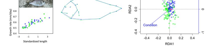
Genes 2020, 11, x FOR PEER REVIEW                                                                              8 of 17
    Genes 2020, 11, 398                                                                                           8 of 17

         Figure 2. Allele frequency changes at 67 outlier loci detected between brackish and marine juveniles
315     with   the single generation selection (SGS) test, using a nominal significance threshold of 10−3 . For
         each locus, allele frequency of the major allele (p) is indicated in the larval pool (red, with the 90%
316           Figure 2. Allele frequency changes at 67 outlier loci detected between brackish and marine juveniles
         credibility interval in grey), brackish juveniles (green triangles) and marine juveniles (blue triangles).
317           with the single generation selection (SGS) test, using a nominal significance threshold of 10-3. For each
         Upper triangles show increased allele frequency compared to the larval pool; lower triangles show
318           locus, allele frequency of the major allele (p) is indicated in the larval pool (red, with the 90%
         decreased allele frequency compared to the larval pool.
319           credibility interval in grey), brackish juveniles (green triangles) and marine juveniles (blue triangles).
320      The Upper    triangles
              PCA based      on show
                                 the 67increased  allele
                                         outlier loci    frequency
                                                      partly         compared brackish
                                                               distinguished  to the larval
                                                                                         andpool; lowerjuveniles
                                                                                             marine      triangles along
                                                                                                                   show
321the first axis,
              decreased   allele frequency  compared    to the larval pool.
                    whereas larvae occupied mostly intermediate positions (Figure S7). The estimation of
    relative survival probability scores in each habitat (Figure 3a,b) revealed that 61.4% of the genotypic
322          The PCA based on the 67 outlier loci partly distinguished brackish and marine juveniles along
   combinations initially present in larvae were found overrepresented in one of the two habitats at the
323    the first axis, whereas larvae occupied mostly intermediate positions (Figure S7). The estimation of
   juvenile stage. This overrepresentation was stronger in the brackish environment, where 45.5% of the
324    relative survival probability scores in each habitat (Figure 3a,b) revealed that 61.4% of the genotypic
   genotypes initially present in the larval pool had a positive survival score, whereas only 15.9% were
325    combinations initially present in larvae were found overrepresented in one of the two habitats at the
   favored in the marine environment. Estimated survival probability scores of larvae in each habitat
326    juvenile stage. This overrepresentation was stronger in the brackish environment, where 45.5% of the
   displayed a moderate trade-off (Figure 3c). The number of brackish alleles per individual (i.e., brackish
327    genotypes initially present in the larval pool had a positive survival score, whereas only 15.9% were
   polygenic score calculated for the 67 outlier loci) was a good predictor of juvenile survival probability
328    favored in the marine environment. Estimated survival probability scores of larvae in each habitat
   scores. Higher brackish polygenic scores were associated with higher survival scores in the brackish
329    displayed a moderate trade-off (Figure 3c). The number of brackish alleles per individual (i.e.,
   habitat but lower survival scores in the marine habitat (Figure 3d; ANCOVA: P = 2.8 × 10⁻¹⁰ , R2 =
330    brackish polygenic score calculated for the 67 outlier loci) was a good predictor of juvenile survival
   0.208; interaction term: P = 6.6 × 10⁻¹¹ ).
331    probability scores. Higher brackish polygenic scores were associated with higher survival scores in
332    the brackish habitat but lower survival scores in the marine habitat (Figure 3d; ANCOVA: P = 2.8 ×
333    10−10,    = 0.208; interaction term: P = 6.6 × 10⁻¹¹).
Genes 2020, 11, 398 9 of 17
Genes 2020, 11, x FOR PEER REVIEW 9 of 17
334
335 Figure 3.
Figure Genotype–fitnessrelationships
3. Genotype–fitness relationshipsassessed
assessedwith
with6767outlier
outlier loci
loci detected
detected with
with the
the SGS
SGS test.
test.
336 Individual coordinates in the two first PCA axes were compared (a) between larvae (red)
Individual coordinates in the two first PCA axes were compared (a) between larvae (red) and brackish and brackish
337 juveniles (green)
juveniles (green) or
or (b)
(b) between
between larvae
larvae and and marine
marine juveniles
juveniles (blue)
(blue) to
to estimate
estimate the
the relative
relative enrichment
enrichment
338 or depletion of multilocus genotypes over the genotypic space (z, the relative survival
or depletion of multilocus genotypes over the genotypic space (z, the relative survival probability probability
339 score surface)
score surface) inin each
each habitat. (c) Estimated
habitat. (c) Estimated survival
survival scores
scores of
of larvae
larvae show
show aa moderate
moderate trade-off
trade-off
340 between habitats. (d) The sum of brackish-favored alleles in individual juveniles is
between habitats. (d) The sum of brackish-favored alleles in individual juveniles is positively positively correlated
341 with survival
correlated withscore in thescore
survival brackish
in the habitat buthabitat
brackish negatively correlated in
but negatively the marine
correlated habitat
in the (ANCOVA
marine habitat
342 interaction term: P = 6.6 × 10 −11 ).
(ANCOVA interaction term: P = 6.6 × 10⁻¹¹).
3.4. Genotype–Phenotype Links
343 3.4. Genotype–Phenotype Links
Only four SNPs showed significant associations at the genome-wide significance level (P < 2.88 ×
344 −5 Only four SNPs showed significant associations at the genome-wide significance level (P < 2.88
10 ) in the GWA study performed for standardized length and condition using three different models.
345 × 10 ) in the GWA study performed for standardized length and condition using three different
−5
Overlaid Q–Q plots for the three models showed that smaller P-values were generally obtained with
346 models. Overlaid Q–Q plots for the three models showed that smaller P-values were generally
the model including genotype-by-environment interaction (Figure S8). Among the 669 loci that were
347 obtained with the model including genotype-by-environment interaction (Figure S8). Among the 669
detected by the SGS test at a nominal significance thresholds of P = 0.01, 15 were found associated
348 loci that were detected by the SGS test at a nominal significance thresholds of P = 0.01, 15 were found
with standardized length and 17 with condition using the same P-value cutoff.
349 associated with standardized length and 17 with condition using the same P-value cutoff.
The proportion of phenotypic variance cumulatively explained by nominally significant variants
350 The proportion of phenotypic variance cumulatively explained by nominally significant variants
detected by the SGS test first increased with decreasing nominal significance thresholds and then
351 detected by the SGS test first increased with decreasing nominal significance thresholds and then
decreased (Figure 4a,c). The amount of explained variance for standardized length was maximized
352 decreased (Figure 4a,c). The amount of explained variance for standardized length was maximized
for a nominal significance threshold of P = 0.0075, at which 495 loci cumulatively explained 3.85% of
353 for a nominal significance threshold of P = 0.0075, at which 495 loci cumulatively explained 3.85% of
phenotypic variation in interaction with habitat using the marine polygenic score (Figure 4b; ANCOVA:
354 phenotypic variation in interaction with habitat using the marine polygenic score (Figure 4b;
P = 0.046; interaction term: P = 6.5 × 10⁻³ ). A similar trend was obtained using measures of mean
355 ANCOVA: P = 0.046; interaction term: P = 6.5 × 10⁻³). A similar trend was obtained using measures of
summer otolith growth rate from 40 juveniles and a nominal significance threshold of P = 0.01 to detect
356 mean summer otolith growth rate from 40 juveniles and a nominal significance threshold of P = 0.01
candidate selected SNPs. However, the significance of the interaction between the marine polygenic
357 to detect candidate selected SNPs. However, the significance of the interaction between the marine
score and habitat was only suggestive (interaction term: P = 0.077) due to a lack of power.
358 polygenic score and habitat was only suggestive (interaction term: P = 0.077) due to a lack of power.Genes 2020, 11, 398 10 of 17
Genes 2020, 11, x FOR PEER REVIEW 10 of 17
359
360 Figure
Figure4. Phenotypic
4. Phenotypic variance
variance explained
explained byby outlier
outlierloci. (a)(a)
loci. The cumulative
The cumulative variance
variance in in
standardized
standardized
361 length
length(y (y axis)
axis) explained
explained byby marine-favored
marine-favored alleles
allelesincreases
increases when
when outlier
outliersingle
single nucleotide
nucleotide
362 polymorphisms
polymorphisms (SNPs)
(SNPs)reaching
reaching lower
lower significance
significance thresholds
thresholds (x (x
axis) areare
axis) included
included in in
thethe
ANCOVA
ANCOVA
363 model
model(interaction
(interaction term: PGenes 2020, 11, 398 11 of 17
Genes 2020, 11, x FOR PEER REVIEW 11 of 17
380
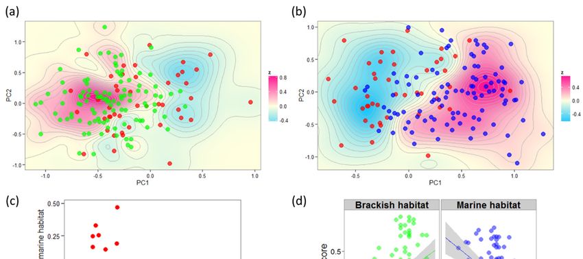
381 Figure 5. Phenotypic
Figure 5. Phenotypicvariance explained
variance explainedby byoutlier lociloci
outlier in the independent
in the independent sample
sampleof of
larvae. (a)(a)
larvae. Picture
382 Picturecollected
of larvae of larvaeoncollected on the
the same day,same day, showing
showing differencesdifferences
in sizeinbetween
size between individuals.
individuals. (b) (b)
Positive
383 Positive (R
correlation correlation
2 = 0.214,( slope
= 0.214,
P= slope P =between
0.01) 0.01) between the average
the average daily
daily widthwidth incrementofofotolith
increment otolith rings
384 during the first 60 days of larval life (y axis, in µm per day) and the marine polygenic score score
rings during the first 60 days of larval life (y axis, in µm per day) and the marine polygenic calculated
385 calculated for the 11 most significant outliers found in the SGS test (x axis, P-value threshold of
for the 11 most significant outliers found in the SGS test (x axis, P-value threshold of 0.0001).
386 0.0001).
4. Discussion
387 4. Discussion
How fitness trade-offs across spatially variable environments translate into population phenotypic
388 How fitness trade-offs across spatially variable environments translate into population
389and genetic responses remains a challenging question in evolutionary biology. Here, we evaluated the
phenotypic and genetic responses remains a challenging question in evolutionary biology. Here, we
390single-generation
evaluated theeffects of dispersal and
single-generation local
effects ofselection
dispersalin and
heterogeneous environments
local selection by comparing
in heterogeneous
391phenotypic and genomic
environments by comparing variation amongand
phenotypic habitats
genomicand life stages
variation among within a single
habitats population
and life stages withincohort of
392gilthead seapopulation
a single bream. cohort of gilthead sea bream.
393 OurOur firstfirst
observation
observationisisthat thatthe the type nurseryhabitat
type of nursery habitatused usedby by juvenile
juvenile fish fish influences
influences the the
394direction
direction of the
of the correlation
correlation betweenindividual
between individual growth
growthraterateandand condition,
condition, which are two
which are important
two important
395fitness-related
fitness-related traits
traits in fish
in fish [32].
[32]. Theseenvironment-dependent
These environment-dependent trait traitcorrelations
correlations arearealso detectable
also detectable at
396the morphometric
at the morphometric level, especially in the marine habitat where
level, especially in the marine habitat where rapid-growth morphologiesrapid-growth morphologies tendtend to
397 to display lower condition. Environmental conditions experienced by juvenile fish strongly influence
display lower condition. Environmental conditions experienced by juvenile fish strongly influence their
398 their growth trajectories, which themselves impact a series of fitness-related traits across the entire
399growth trajectories, which themselves impact a series of fitness-related traits across the entire life cycle
life cycle (e.g., juvenile mortality, timing of winter migration at sea, survival to sexual maturity,
400(e.g.,reproduction).
juvenile mortality,
Although timing of winter
selection should migration
generally at sea,higher
favor survival to sexual
juvenile growth maturity, reproduction).
rates to maximize
401Although selection should generally favor higher juvenile growth
survival and reproduction, fast growth can be sometimes associated to physiological, developmentalrates to maximize survival and
402reproduction,
and ecologicalfast conditions
growth can thatbeinduce
sometimesfitnessassociated to physiological,
costs [45]. For instance, elevated developmental
growth rates can and ecological
reduce
403conditions
the juveniles' ability to
that induce endure
fitness periods
costs [45].ofForstarvation,
instance, which are typically
elevated growthmore ratesfrequent
can reducein thethe
marine
juveniles’
404ability
environment. Therefore,
to endure periods of the optimal growth
starvation, which are strategy may more
typically change according
frequent to habitat
in the marinetype, and
environment.
405Therefore,
different growth strategies that are genetically encoded may evolve and
the optimal growth strategy may change according to habitat type, and different growth segregate in the population
406strategies
in response to fitness trade-offs between habitats.
that are genetically encoded may evolve and segregate in the population in response to
407 Although the phenotypic correlations observed here may partly reflect environmentally induced
fitness trade-offs between habitats.
408 plasticity, they also mirror environment-dependent genetic correlations that have been already
409 Although the phenotypic correlations observed here may partly reflect environmentally induced
observed between growth and condition in experimental conditions [46]. These correlations also
410plasticity, they also
correspond mirror environment-dependent
to long-term evolutionary responses that genetic
have correlations
been associated that have
with been already
different observed
life-history
411between growth
strategies and condition
in fishes. In general,in experimental
species that occurconditions
in unstable but[46].highly
These correlations
productive also correspond
environments like to
412long-term
brackish evolutionary
lagoons tendresponsesto show higher that have beengrowth
juvenile associated
rates with differentindices
and condition life-history
comparedstrategies
to in
413fishes.
marine species occupying
In general, species that more stableinbut
occur less productive
unstable environments
but highly productive [47].environments
Therefore, the sea beam
like brackish
414lagoons
that tend
uses both habitat types at the juvenile stage may face trade-offs between
to show higher juvenile growth rates and condition indices compared to marine species growth and other life-
415occupying
history more
traits stable
due to butvarying environmental
less productive constraints
environments among
[47]. nursery
Therefore, thehabitats.
sea beam Thisthatraises
uses both
416habitat
interesting questions about maintenance of variation at loci affecting survival in each environment.
types at the juvenile stage may face trade-offs between growth and other life-history traits due
417 Growth rate and condition are both complex polygenic traits with moderate to high heritable
to varying environmental constraints among nursery habitats. This raises interesting questions about
418 components in sea bream [48,49]. These traits are also genetically correlated [46,49] and are therefore
419maintenance of variation at loci affecting survival in each environment.
possibly encoded by partially overlapping sets of genes. If selection underlies the environment-
420 Growth rate
dependent and
trait conditionobserved
correlations are both here, complex this polygenic
should involvetraitsmutations
with moderate to high heritable
with environment-
components in sea bream [48,49]. These traits are also genetically correlated [46,49] and are
therefore possibly encoded by partially overlapping sets of genes. If selection underlies the
environment-dependent trait correlations observed here, this should involve mutations withGenes 2020, 11, 398 12 of 17
environment-dependent pleiotropic effects, that is, genotype–environment interactions [50,51]. Here,
conditionally neutral mutations and mutations with antagonistic fitness effects across environments [9]
were searched by explicitly considering the single-generation footprint of selection in panmixia. As for
other statistical approaches based on single-locus tests, our method lacks the power to detect very small
allele frequency changes caused by selection. This limitation is however potentially compensated for by
the prediction that, in high gene flow species, local selection in spatially heterogeneous environments
tends to favor polygenic architectures characterized by a high variance in locus effect size [3,22]. If this
prediction is verified, even in the presence of false positives, our approach should at least detect the
fraction of loci that contribute the most to differential survival in the fraction of the genome tagged by
our RAD markers.
The fitness effects of candidate outlier SNPs were evaluated both individually and collectively. In
both cases, comparisons between pre- and postselection samples revealed that groups of juveniles from
different environments depart in opposite directions from their larval pool of origin. This suggests
that recruitment to brackish and marine nurseries is random with respect to the ability of larvae to
succeed in a given environment. Under the alternative hypothesis of habitat selection, our larval
sample collected at the entrance of the Thau lagoon would be expected to show more genetic proximity
to marine juveniles at outlier loci, which is not what we observed (we actually found a trend in the
opposite direction). This clearly rejects the matching habitat choice hypothesis, which was already
dismissed in earlier works in sea bream [30]. Therefore, the subtle changes in allele frequency detected
here most likely reflect the action of spatially varying polygenic selection spread across multiple
loci [13,52]. Interestingly, our results suggest that selection generates softer allele frequency changes in
the brackish environment, which is the most abundant habitat type used by the majority of juveniles
in the studied region [27,53]. The mean fitness of the population is therefore probably closer to the
optimum of the brackish environment, as illustrated by survival probability score surfaces and by
the fact that twice as many larvae have a positive survival score in the brackish compared to the
marine environment. In species like sea bream, density regulation should mainly occur within nursery
habitats, such that each habitat has a constant contribution to the next generation that reflects its
carrying capacity [1]. Under weak to moderate trade-offs, this type of life cycle is known to favor
the evolution of a single generalist showing intermediate local adaptation biased toward the most
abundant and productive habitat [54]. Our results are consistent with this theoretical prediction. A
limitation, though, could be the lack of replication compared to other study designs in similar studies
(e.g., [25]). Our study only includes a single sample from each of the two alternative juvenile habitats,
which is not enough to fully demonstrate that the differences observed are due to the environmental
differences between marine and brackish habitats. Therefore, the relationships detected here cannot be
extended beyond the two study sites at the present time and will need further investigations.
Our next objective was to evaluate the extent to which candidate SNPs for spatially varying
selection explained phenotypic variation among individuals and environments. GWA analyses revealed
that individual variants explain at most a small and usually insignificant fraction of phenotypic variance.
Therefore, there is a limited overlap between the list of candidate SNPs for spatially varying selection
and candidate loci detected in our GWA study. To compensate for this lack of power, we used additive
polygenic scores to estimate the joint contribution of candidate variants to phenotypic variation. This
approach has already provided informative assessments of polygenic gene action on fitness-related
traits [23,24]. It is however intrinsically constrained by the statistical threshold used for candidate SNP
detection in single locus tests. GWA studies for complex traits in humans have dealt with this issue
using decreasing significance thresholds to progressively include additional smaller-effect candidate
variants in polygenic scores [55,56]. Here, we adopted a similar strategy by evaluating the amount of
phenotypic variance collectively explained by candidate outlier SNPs that were detected without taking
phenotypic information into account, under different significant thresholds. Although this approach
may be prone to false-positive detection of candidate SNPs for selection, false positive outliers are
unlikely to contribute to phenotypic variance by chance, thus insuring an independent assessmentGenes 2020, 11, 398 13 of 17
of the additive effect of outlier SNPs on phenotype in interaction with environment. Moreover, the
correlation detected between the marine polygenic score and larval growth rate indicated that false
positive detection was not a major issue. Indeed, outlier loci were only searched using juvenile samples,
and therefore the larval sample provided a completely independent support that at least some of
the detected genes are truly involved in the studied phenotypes. These results also indicate that
larval growth and juvenile growth are controlled by partially overlapping sets of genes, which is
not surprising.
Overall, our results provide empirical support that selected variants with moderate to small
individual effects on fitness traits can cumulatively explain several percent of the phenotypic variance
among individuals living in contrasted environments. More generally, they support the view that
selected mutations with antagonistic pleiotropic effects partly underlie the environment-dependent
correlations between growth and condition in juvenile sea bream.
Antagonistic pleiotropy between environments likely involves complex allocation trade-offs that
emerge due to compromises between growth and stress regulation [57,58]. Juvenile sea bream are
subject to different sources of stress, ranging from highly unstable conditions in brackish lagoons
to frequent starvation in the marine environment [26]. This supposes the existence of different
optimal growth trajectories among environments, because the fast-growing genotypes favored in rich
habitats are not the best adapted to poor habitats, where they are unable to cope with prolonged food
deprivation. The well-studied phenomenon of compensatory growth [59] illustrates the necessity
for fish to perform growth regulation to buffer unpredictable environmental variation. In juvenile
sea bream, the environment-dependent correlation between growth and condition may thus reflect
selection for different growth trajectories in relation with food availability and stress.
Reduced genome representation methods such as RAD-Seq have been criticized as providing
insufficiently dense genome-scans for detecting local adaptation genes when linkage disequilibrium
extends over small chromosomal distances around selected loci [60–62]. We acknowledge that we
have most probably missed a number of selected loci, possibly some with larger effects than those
we detected. This can be explained by several reasons, including imperfect linkage disequilibrium of
marker loci with the causative variants, or the existence of rare variants of large effect and especially
of many small effect-size loci that cannot be detected with the limited sample sizes used in this
study. This drawback adds to the issue discussed above that even intermediate-effect variants are
expected to display small allele frequency differentials between habitats. However, our approach
allowed quantifying the proportion of phenotypic variance explained by the candidate outlier loci [19],
which proved to be non-negligible. In line with previous studies [63,64], we therefore argue that
the cost-effective approach implemented here provides sufficient marker density to get access to a
meaningful fraction of the genetic variance for fitness traits.
5. Conclusions
To conclude, the molecular footprint of local polygenic selection acting within a single generation
was found at multiple SNPs, which will need to be further validated using a recently developed
high-density SNP array in the gilthead sea bream. Our results imply that fitness-related traits such as
juvenile growth and condition are encoded by multiple small-effect genes with antagonistic pleiotropic
effects across environments. They also support the view that different life-history strategies, which are
partly genetically encoded, segregate in sea bream as a response to different optimal growth trajectories
across juvenile habitats.
Supplementary Materials: The following are available online at http://www.mdpi.com/2073-4425/11/4/398/s1,
Figure S1: Distribution of per-individual read counts that were retained after quality filtering, Figure S2: Parameter
optimization for Stacks, Figure S3: The prior probability distribution of Z in the common gene pool. Figure S4:
The posterior probability distribution of Z in the common gene pool, Figure S5: Assessment of the power of
the Bayesian test to detect single-generation selection in comparison to Fisher’s exact test. Figure S6: Principal
Component Analysis performed for each of the two datasets, Figure S7: Principal Component Analysis performed
on the outlier SNP dataset (67 SNPs from Figure 2), Figure S8: Genome-wide association analysis performed forGenes 2020, 11, 398 14 of 17
standardized length (a) and condition (b). Table S1: Sampling details, Table S2: Pairwise genetic differentiation
(FST ) among the three samples based on two different polymorphism datasets (SNPs, haplotypes). Supplementary
Methods: Test for single-generation selection. Data Accessibility: Data supporting the results will be deposited
under GenBank SRA and Dryad upon acceptance.
Author Contributions: P.-A.G. conceived and designed the study with inputs from B.G., F.B. and N.B. P.-A.G.
and C.R. collected and analyzed phenotypic and molecular data. A.D. and F.F. collected and analyzed otolith data.
P.-A.G. and C.R. drafted the initial version of the manuscript and all authors contributed to later versions of the
manuscript. All authors have read and agreed to the published version of the manuscript
Funding: This research was funded by the CNRS-INEE Appel à Projets En Génomique Environnementale - APEGE
2013, grant number ArchiGen BFC 78167. The APC was funded by CNRS.
Acknowledgments: We thank M-T Augé and A Souissi for their precious help with RAD library construction.
We also thank three anonymous reviewers for their insightful comments on the manuscript. Fish collection and
otolith processing for this work were supported by the CNRS INEE EC2CO project METASPAR (PI: D. Mc Kenzie)
and by the BOUCLEDOR project co-funded by the European Regional. Development Fund and the French
Languedoc-Roussillon Region (FEDER FSE IEJ 2014-2020, PI: A Darnaude). We are grateful to Chloé Vagnon for
her assistance in otolith data acquisition.
Conflicts of Interest: The authors declare no conflict of interest. The funders had no role in the design of the
study; in the collection, analyses, or interpretation of data; in the writing of the manuscript, or in the decision to
publish the results.
References
1. Levene, H. Genetic Equilibrium When More Than One Ecological Niche is Available. Am. Nat. 1953, 87,
331–333. [CrossRef]
2. Levins, R. Evolution in Changing Environments: Some Theoretical Explorations; Princeton University Press:
Princeton, NJ, USA, 1968.
3. Lenormand, T. Gene flow and the limits to natural selection. Trends Ecol. Evol. 2002, 17, 183–189. [CrossRef]
4. Hedrick, P.W. Genetic Polymorphism in Heterogeneous Environments: The Age of Genomics. Annu. Rev.
Ecol. Evol. Syst. 2006, 37, 67–93. [CrossRef]
5. Chevin, L.-M.; Lande, R.; Mace, G.M. Adaptation, plasticity, and extinction in a changing environment:
Towards a predictive theory. PLoS Boil. 2010, 8, e1000357. [CrossRef] [PubMed]
6. Sgrò, C.M.; Lowe, A.; Hoffmann, A.A. Building evolutionary resilience for conserving biodiversity under
climate change. Evol. Appl. 2010, 4, 326–337. [CrossRef] [PubMed]
7. Funk, W.C.; McKay, J.K.; Hohenlohe, P.A.; Allendorf, F.W. Harnessing genomics for delineating conservation
units. Trends Ecol. Evol. 2012, 27, 489–496. [CrossRef] [PubMed]
8. Harrisson, K.A.; Pavlova, A.; Telonis-Scott, M.; Sunnucks, P. Using genomics to characterize evolutionary
potential for conservation of wild populations. Evol. Appl. 2014, 7, 1008–1025. [CrossRef]
9. Savolainen, O.; Lascoux, M.; Merilä, J. Ecological genomics of local adaptation. Nat. Rev. Genet. 2013, 14,
807–820. [CrossRef]
10. Grummer, J.A.; Beheregaray, L.B.; Bernatchez, L.; Hand, B.; Luikart, G.; Narum, S.R.; Taylor, E.B. Aquatic
Landscape Genomics and Environmental Effects on Genetic Variation. Trends Ecol. Evol. 2019, 34, 641–654.
[CrossRef]
11. Barrett, R.D.H.; Hoekstra, H.E. Molecular spandrels: Tests of adaptation at the genetic level. Nat. Rev. Genet.
2011, 12, 767–780. [CrossRef]
12. Wellenreuther, M.; Hansson, B. Detecting Polygenic Evolution: Problems, Pitfalls, and Promises. Trends
Genet. 2016, 32, 155–164. [CrossRef] [PubMed]
13. Pritchard, J.K.; Di Rienzo, A. Adaptation – not by sweeps alone. Nat. Rev. Genet. 2010, 11, 665–667. [CrossRef]
[PubMed]
14. Rockman, M.V. THE QTN PROGRAM AND THE ALLELES THAT MATTER FOR EVOLUTION: ALL
THAT’S GOLD DOES NOT GLITTER. Evolution 2011, 66, 1–17. [CrossRef] [PubMed]
15. Goddard, M.; Hayes, B. Mapping genes for complex traits in domestic animals and their use in breeding
programmes. Nat. Rev. Genet. 2009, 10, 381–391. [CrossRef]
16. De Villemereuil, P.; Frichot, É.; Bazin, E.; François, O.; Gaggiotti, O.E. Genome scan methods against more
complex models: When and how much should we trust them? Mol. Ecol. 2014, 23, 2006–2019. [CrossRef]You can also read