Linking Nature in the City - Part Two - Applying the Connectivity Index Holly Kirk, Caragh Threlfall, Kylie Soanes, Kirsten Parris - The Clean ...

Linking Nature in the City – Part
Two

Applying the Connectivity Index
Holly Kirk, Caragh Threlfall, Kylie Soanes, Kirsten Parris.

May 2020

About the Clean Air and Urban Landscapes Hub
The Clean Air and Urban Landscapes Hub (CAUL) is a consortium of four universities: the
University of Melbourne, RMIT University, the University of Western Australia and the
University of Wollongong. The CAUL Hub is funded by the Australian Government’s
National Environmental Science Program. The task of the CAUL Hub is to undertake research
to support
environmental quality in our urban areas, especially in the areas of air quality, urban greening,
liveability and biodiversity, and with a focus on applying research to develop practical solutions.

www.nespurban.edu.au

Acknowledgements
We acknowledge the Traditional Custodians of the land where this research took place, and pay
our respects to Elders past, present and emerging. We are very grateful to the City of Melbourne
for funding this project. We would especially like to thank members of the Urban Sustainability
Branch for making this exciting research possible. We thank the researchers involved in Part 1
(Kirk et al. 2018) upon which this work builds. We would also like to thank Dr Nick Golding for
his assistance setting up the RStudio servers needed to complete this work and his useful
comments on the methodology. This research was supported by the Australian Government’s
National Environmental Science Program and the Nectar Research Cloud, a collaborative
Australian research platform supported by the Australian Research Data Commons (ARDC) and
National Collaborative Research Infrastructure Strategy (NCRIS).

Please cite this document as:
Kirk H., Threlfall C., Soanes K. & Parris, K. (2020) Linking Nature in the City Part Two: Applying
the Connectivity Index. Report prepared for the City of Melbourne Urban Sustainability Branch.

The Clean Air and Urban Landscapes Hub is funded by the Australian Government's
National Environmental Science Program

Executive Summary

Building on the Linking Nature in the City: A framework for improving ecological
connectivity across the City of Melbourne project (Kirk et al, 2018), this report (Linking
Nature in the City – Part Two) summarises findings and guidance for applying
ecological connectivity theory to the City of Melbourne’s capital works. It tests the
sensitivity of the connectivity index to underlying assumptions about animal movement
across an urban landscape. It also demonstrates how the connectivity index can be
used to prioritise road segments to be targeted for biodiversity-focussed actions as the
City of Melbourne works to achieve targets laid out in its Nature in the City Strategy
(2017).

The connectivity index depends on three main parameters, which are contingent on
the species being considered: the area and spatial arrangement of habitat patches in
the focal landscape, the spatial arrangement of barriers to movement, and the
movement capability of the target species. Movement ability of the target species
translates to the threshold distance at which habitat patches are connected for that
species. Barriers to movement are physical obstacles that cannot be crossed by the
species in question. These barriers include roads of different widths or vehicle activity,
buildings, or areas that could be inhospitable such as expanses of open ground,
concrete or saltwater. To understand the response of the connectivity index to differing
parameter inputs, we kept the area of habitat constant and incrementally changed the
threshold distance or road-barrier definition and re-calculated the index each time. We
did this for the seven species groups introduced in Part One (reptiles, amphibians,
insect pollinators, aquatic insects, tree-hollow using birds, tree-hollow using bats and
woodland birds).

Testing the sensitivity of the connectivity index to these parameters showed that
careful consideration is needed when applying the index to different animal species. If
the movement ability of the target species is uncertain, the estimated minimum and
maximum movement ability should always be used in order to produce a range of
estimates of ecological connectivity. The analysis undertaken here showed that the
distance parameters based on mean or median movement ability used in the Linking
Nature in the City – Part One were too generous. When the connectivity index was
tested for varying road barrier definitions it showed the greatest variation between
roads wider than 7m and roads wider than 20m. Again, this indicates that if there is

 Page 1

uncertainty about how a target species responds to road width, then the connectivity
index should be calculated for the range of possible values.

We modelled removing the barrier effect of each road segment in the City of Melbourne
to understand the impact of each road segment on the ecological connectivity of the
city. The consequent increase in the connectivity index could be compared for all road
segments, which allowed us to rank each road segment across the City of Melbourne.
We have identified the Top 10 roads to prioritise for biodiversity-focussed actions in
order to improve ecological connectivity for each of the seven target species. Road-
based works aimed at improving ecological connectivity should focus on mitigating the
barrier effect of the road through actions such as street planting and narrowing or
traffic calming.

Top 10 Roads with segments to target for improving overall ecological connectivity:

 1 Government House Drive
 2 Hotham Street
 3 Old Poplar Road
 4 St Kilda Road
 5 Linlithgow Avenue
 6 Morell Bridge
 7 Swanston Street
 8 Simpson Street
 9 Birdwood Avenue
 10 Docklands Drive

 Page 2

Contents

Executive summary Page 1

1. Introduction and methods Page 4

2. Results Page 8

 Activity 1 – Sensitivity testing Page 8

 Activity 2 – Ranking roads Page 21

3. Recommendations Page 29

4. Detailed methodology Page 34

5. References Page 38

 Page 3

1. Introduction and methods

Ecological connectivity & the City of Melbourne
The City of Melbourne has made a commitment to enhance the liveability of the City
by encouraging urban nature and supporting “diverse, resilient, and healthy
ecosystems” (Nature in the City Strategy, 2017). A key target within this Strategy was
“by 2027, City of Melbourne will be a more ecologically-connected city than in 2017”.
Ecological connectivity, the degree to which a landscape facilitates or impedes the
movement of an organism, is a fundamental concept in conservation science and is
increasingly being applied to a range of environments to measure species return and
persistence (Bunn et al., 2000; Taylor et al., 1993; Tischendorf & Fahrig, 2000). Many
animal species need to move or disperse for several reasons: to find food, water or
shelter, for reproductive opportunities and after breeding to establish new territories
(Baguette et al., 2013, 2014; Brooker et al., 1999; Chisholm et al., 2011). Measuring
ecological connectivity quantifies the spatial arrangement of habitat or resources
within a landscape, accounting for barriers to movement, and allows practitioners to
compare the potential effects of different planning scenarios on populations (Beier et
al., 2011; Bunn et al., 2000; Correa Ayram et al., 2016; LaPoint et al., 2015; Loro et
al., 2015). By considering ecological connectivity in their environmental planning, the
City of Melbourne is intending that the strategies they use to improve urban nature
result in thriving, stable wildlife populations.

The 2018 report Linking Nature in the City: A framework for improving ecological
connectivity across the City of Melbourne outlined a framework for quantifying
ecological connectivity within urban landscapes, focussing on animal species. The
framework details a GIS-based workflow to allow the City of Melbourne to assess
existing ecological connectivity and determine the effect of different development
scenarios. Linking Nature in the City: A framework for improving ecological
connectivity across the City of Melbourne (hereafter Linking Nature in the City – Part
One) quantified connectivity for seven animal groups, each of which could act as an
“umbrella” for several species occurring within Greater Melbourne (Table 1).

Species groups and example members:
Amphibians (e.g. spotted marsh frog Limnodynastes tasmaniensis)
Reptiles (e.g. Eastern blue-tongue lizard Tiliqua scincoides)
Insect pollinators (e.g. blue-banded bee Amegilla sp.)
Aquatic insects (e.g. blue skimmer dragonfly Orthetrum caledonicum)
Tree-hollow using birds (e.g. red-rumped parrot Psephotus haematonotus)
Tree-hollow using bats (e.g. Gould’s wattled bat Chalinolobus gouldii)
Woodland birds (e.g. superb fairywren Malarus cyaneus)

 Page 4

There are several ways to quantify ecological or landscape connectivity (Calabrese &
Fagan, 2004; Correa Ayram et al., 2016; Kindlmann & Burel, 2008). The approach
used in Linking Nature in the City - Part One was chosen as it 1) allowed comparisons
over time and between different cities and 2) could be implemented by the City of
Melbourne’s in-house GIS team using existing vector-based spatial data (Jaeger et
al., 2008; Deslauriers et al., 2018). The measure of ecological connectivity (the
connectivity index), used in Linking Nature in the City – Part One and here, is based
on the geometric measure of effective mesh size ( eff ), a method that quantifies the
degree to which patches of habitat are fragmented. Effective mesh size compares the
number of groups of connected habitat patches against the total area of habitat within
the landscape (see section 4 for more details; (Deslauriers et al., 2018; Spanowicz &
Jaeger, 2019). The connectivity index (m_eff) represents the average amount of
habitat available to an individual animal placed anywhere into the landscape (Jaeger,
2000; Spanowicz & Jaeger, 2019).

Sensitivity of the connectivity index
A sensitivity analysis explores how the output from a model is affected by varying each
of the input parameters used within the model. When estimating ecological
connectivity using the connectivity index described here, the model uses three types
of data: a spatial polygon of available habitat for the target species, a spatial polygon
of potential barriers to movement and an estimate of the dispersal capability (in
metres) of the target species. Dispersal capability informs the distance threshold used
to determine if patches of habitat are “connected” or not. Background ecological
knowledge for each target species is used to identify their appropriate habitat types,
potential movement barriers and the average dispersal capability, although these
pieces of information are not always known for the species in question. The data used
for each species group in Linking Nature in the City – Part One are described briefly
here (Table 1). There is some uncertainty within all three of the data inputs:
 o Habitat uncertainty: has the required habitat been correctly identified
 and is the spatial information accurate?
 o Barrier uncertainty: have appropriate barriers to movement been
 identified? These are usually roads, railways and or buildings depending
 on the target species.
 o Distance uncertainty: has the dispersal capability (or gap-crossing
 ability) of the target species been recorded empirically? How big is the
 range in possible distance values, and should the mean or median be
 used? If no empirical evidence is available for the target species, what
 alternatives are available?

 Page 5

Table 1. Input data used to estimate the connectivity index across the City of Melbourne for seven
animal groups in Linking Nature in the City - Part One.
 Distance
 Group Habitat threshold Barriers
 (m)
 Understorey vegetation and turf Roads > 5m, all
 Amphibians 1000
 near water buildings
 Mid- & understorey vegetation Roads > 5m, all
 Reptiles 1000
 and turf buildings
 Mid-storey vegetation and trees,
 Insect pollinators 350 Roads > 10m
 nearby turf
 Water and all vegetation close to
 Aquatic insects 1500 Roads > 10m
 water
 Tree-hollow using Turf and canopy close to hollow- Roads > 15m,
 500
 bird bearing trees buildings > 10m
 Tree-hollow using Canopy close to hollow-bearing Roads > 15m,
 1000
 bats trees buildings > 10m
 All canopy and mid-storey
 Roads > 15m,
 Woodland birds vegetation, turf close to 1500
 buildings > 10m
 vegetation

To understand the sensitivity of the connectivity index to changes in these input
parameters, we changed one input parameter at a time then re-calculated the index
using R 3.6.0, an open source software for statistical computing (R Core Team, 2019).
This facilitated the many hundreds of repeated calculations of the connectivity index
needed to test the sensitivity of the model.

To investigate the effect of changing distance threshold, we calculated the connectivity
index for each of the seven species groups and varied the assumed dispersal
capability for each group from 5 m to 1800 m in 10 m increments. The distance
parameter represents how large a gap in habitat needs to be before patches can no
longer be considered as “connected”. For species that cannot move very far, habitat
patches need to be closer together, while species that can move larger distances may
cross larger gaps between habitat patches. In this analysis, the area of available
habitat was held constant for each species group, as were any barriers to movement.

In this definition of ecological connectivity, two patches of habitat are considered
“connected” if they are not separated by a barrier to movement, such as a road, river,
railway or building. In Linking Nature in the City – Part One we used three different
definitions of what could be considered a road barrier: roads wider than 5 m, 10 m or
15 m. This depended on the focal species group (amphibians and reptiles would
struggle to cross a road wider than 5 m, whereas birds may cross a road wider than
15 m). To look at how varying the road-barrier definition affects the connectivity index,
we calculated the index using a variety of different road widths: roads wider than 3 m,
> 5 m, > 7 m, > 10 m, > 15 m, > 20 m, > 25 m and > 30 m. We also calculated the
connectivity index where all roads in the City of Melbourne were considered barriers.

 Page 6

The area of habitat and the distance threshold (100 m) were kept constant. For this
analysis, we did not consider different animal groups separately but used all vegetation
layers as the definition of habitat. This is consistent with the “structural connectivity”
definition used in Linking Nature in the City – Part One.

Contribution of roadways to connectivity
Consultation with the City of Melbourne indicated that roads are key spaces where the
City can act to improve ecological connectivity. This could be through various actions
including enhancing existing roadside habitat and managing traffic. In order to target
these actions towards road segments with the greatest potential to improve ecological
connectivity, we compared the change in connectivity index across road segments,
allowing us to provide an overall ranking.

We calculated the connectivity index for all seven species groups, based on existing
habitat availability, the lowest estimated inter-patch movement distance (from Activity
1) and the same barrier & habitat definitions as in Linking Nature in the City - Part One
(see Table 1). We then modelled scenarios where the barrier effect of each road
segment was removed to allow the different animal groups to cross. We did this by
first excluding all road segments that were labelled as either “Arterial”, “Port roads”,
“Freeway”, “Citylink”, “Lease/Reserve”, “Private” or “Intersection”. Intersection
segments are very small areas in the middle of four different road segments, rather
than an actual stretch of road. The remaining roads were then grouped according to
three width classes, wider than 5 m (1283 roads), wider than 10 m (648 roads) and
wider than 15 m (110 roads), corresponding to the different barrier definitions for
different animal groups. We then incrementally removed each road segment (to model
the removal of its barrier effect) and re-calculated the connectivity index. For each road
segment, its contribution to the landscape measure of connectivity was measured by
the difference between the initial connectivity index and the one calculated after its
removal.

 Page 7

2. Results

Activity 1 – Sensitivity of the connectivity index to varying inputs
Distance threshold
The distance parameter in estimations of ecological connectivity corresponds to the
ability of an animal to cross gaps between suitable habitat patches. The further a
species can move (the longer its dispersal capability), the wider the gap in habitat it
can cross, which means that patches that are further apart can still be classified as
“connected”. We tested the relationship between assumed dispersal distance and the
connectivity index by keeping the habitat availability and barrier definition (see Table
1) constant for each animal group and varying the threshold distance from 5 m to 1800
m.

Figure 1 illustrates how the connectivity index changes with assumed dispersal
distance for each species across this range. The connectivity index increases as the
threshold distance increases; however, it does this in a stepwise manner. This is
because, as the distance threshold increases, some larger habitat patches become
“connected” (e.g. parks) leading to a big increase in the overall connected area. This
stepwise change in connectivity shows that the index is very sensitive to changes the
distance threshold. Therefore, the threshold distance used to calculate connectivity for
a species needs to be robust. If there is uncertainty in the animal’s movement ability,
then using the estimated lowest and highest values would allow for better evaluation
of the range in connectivity index (Table 2, Figures 1 & 2). This will prevent under- or
over-estimation of the connectivity index for a species and is especially important for
species where movement ability might vary across shorter distances (1 m - 200 m,
appearing as steep slopes in Figure 1). The range in connectivity index values across
the range in species movement estimates can be compared in Figure 2.

In Linking Nature in the City – Part One a single mean or median distance was used
to estimate connectivity for each animal group. These average values were taken from
empirical studies on similar species; however, these studies frequently showed a
range in recorded movement abilities (Table 2, Figure 2). Figure 3 shows the distance-
connectivity curves for each of the seven animal groups in separate plots. Each plot
has a black dot which represents the distance threshold originally used in Linking
Nature in the City – Part One of the project and a shaded area showing the range in
distances recorded in the literature. This range was sometimes very large, for example
different bat species were recorded moving between 100 and 8500 m (Lumsden et al.,
2002; Threlfall et al., 2013) and dragonflies have been recorded migrating more than
100km (Theischinger & Hawking, 2016). A more extensive literature review has
revealed that our earlier estimates of average distance moved were too generous for

 Page 8

the reptile species group. This highlights the need to consider movement over much
 shorter distances.

 The stepwise change in connectivity is spatially visualised in Figure 4, where a pair of
 maps have been created for each animal group across the range in movement
 distances (lowest and highest values). Black boxes indicated places where several
 large areas of habitat have become “connected” as the distance increases (shown by
 a change from two/three different colours to all being the same colour).

 Table 2. Summary of information used to determine the dispersal capability of each animal group, the
 original distance threshold used in Linking Nature in the City – Part One, the range of distances taken
 from the literature and corresponding range in connectivity values.
 Original Distance
 Distances in Connectivity Connectivity
Group distance range tested References
 literature Index Index range
 (m) (m)
 (Berven &
 Growling grass frog Grudzien, 1990;
 min 1196m (mark- 0.292 – 2014;
 1500 0.312 400-1200
insects recapture); other 0.312 Southwood,
 studies report “many 1962)
 miles” for migration.

 Regent parrot colony
 (Baker-Gabb &
 range 50m-9km; red-
 Hurley, 2011);
 rumped parrot
Tree-hollow 0.457 – (Lowry & Lill,
 minimum 10m; ground 500 0.473 100-500
using birds 0.473 2007);
 parrot home range
 (McFarland,
 9.2Ha, flight distance
 1991)
 90-450m.

 Page 9

Gould’s long-eared bat
 max distance from (Threlfall et al.,
Tree-hollow 0.357 –
 roost 111-284m; 1000 0.523 100-1200 2013; Lumsden
using bats 0.523
 Gould’s wattled bat 4- et al., 2002)
 10km

 Superb fairywren
 dispersal distance
 500m – 5km; various
 species wide gaps (Lees & Peres,
 >70m; Eastern 2009; Garrard
Woodland 0.479 –
 spinebill 460m; red 1500 0.852 200-1200 et al., 2012;
birds 0.852
 wattlebird 1.3km; Harrisson et al.,
 spotted pardalote 2013)
 1.2km; brown-headed
 honeyeater 280m;
 golden whistler 1.5km

 Table 2 (cont). Summary of information used to determine the dispersal capability of each animal
 group, the original distance threshold used in Linking Nature in the City – Part One, the range of
 distances taken from the literature and corresponding range in connectivity values.

 Page 10

Figure 1. Effect of changing distance threshold on the connectivity index, presented here as a probability of any two patches being connected (effective mesh
size divided by the total area of habitat) for all seven animal groups. The black dot shows the original distance threshold used in Linking Nature in the City -
Part 1.

 Page 11

Figure 2. The range in connectivity estimates for each animal group. The line shows the connectivity
estimates calculated for the min and max distances taken from the literature. The dot shows the
connectivity value for the distance threshold originally used in Linking Nature in the City - Part 1.

 Page 12

Figure 3. Effect of inter-patch distance threshold on the probability of connectedness (effective mesh
size divided by the total area of habitat) for the amphibian, reptile and insect pollinator groups. The grey
shaded area shows the range of estimated dispersal distances taken from the literature. The black dot
shows the original distance threshold used in Linking Nature in the City - Part 1.

 Page 13

Figure 3 (continued). Effect of inter-patch distance threshold on the probability of connectedness
(effective mesh size divided by the total area of habitat) for the aquatic insect, tree-hollow using bird
and tree-hollow using bat groups. The grey shaded area shows the range of estimated dispersal
distances taken from the literature. The black dot shows the original distance threshold used in Linking
Nature in the City - Part 1.

 Page 14

Figure 3 (continued). Effect of inter-patch distance threshold on the probability of connectedness
(effective mesh size divided by the total area of habitat) for the woodland bird group. The grey shaded
area shows the range of estimated dispersal distances taken from the literature. The black dot shows
the original distance threshold used in Linking Nature in the City - Part 1.

 Page 15

Figure 4. Maps illustrating the difference between using high and low distance thresholds to estimate
connectivity. These show the available habitat for amphibian, reptile and insect pollinator groups
coloured according to patch ID. Connected patches are shown in the same colour, unconnected
patches in different colours. The higher distance-threshold maps are on the right, with a box highlighting
where patches have become classified as “connected” as the predicted gap-crossing ability of the
animal group has increased.

 Page 16

Figure 4 (continued). Maps illustrating the difference between using high and low distance thresholds
to estimate connectivity. These show the available habitat for tree-hollow using bird, bat and woodland
bird groups coloured according to patch ID. Connected patches are shown in the same colour,
unconnected patches in different colours. The higher distance-threshold maps are on the right, with a
box highlighting where patches have become classified as “connected” as the predicted gap-crossing
ability of the animal group has increased.

 Page 17

Effect of road width
To examine the effect of road width on the connectivity index we combined all
vegetation layers and used a 100m distance threshold. These inputs were the same
as those used in Linking Nature in the City – Part One for the overall “structural
connectivity” assessment. These parameters for habitat and threshold distance are
analogous to those originally used in the City Biodiversity Index (Singapore Index)
method for measuring connectivity (Deslauriers et al., 2018). Nine different definitions
of “barrier” were then used to calculate the connectivity index: all roads, then roads
wider than 3 m to roads wider than 30 m (in 2 – 5 m increments).

The connectivity index increases as fewer, wider roads are defined as barriers (Figure
5). The steepest slope in this relationship occurs between roads wider than 7m and
roads wider than 20m. The relationship plateaus after only roads wider than 20m are
used, but this is because there are very few (< 10) roads in the City of Melbourne that
meet this definition. The definition of road barriers used Linking Nature in the City –
Part One ranged from roads wider than 5m to roads wider than 15m. This band falls
into the steepest part of Figure 5, indicating that if there is any uncertainty about what
width of road would act as a barrier for an animal species, then the range in possible
barrier values should be used.

Figure 5. Effect of road barrier definition on the connectivity index (given here as effective mesh size).
This represents the range of road widths present in the City of Melbourne.

 Page 18

Traffic volume and road width
We hypothesised that traffic volume was related to road width. The City of Melbourne
provided a traffic-volume dataset for a subset of their roads. We summarised mean
total daytime and night-time traffic volume for each road and then matched these using
the segment ID to the road spatial layer (containing road width information). Of the
>4000 road segments within the road layer, only 169 had traffic volume information.
Hence, it was not possible to carry out a connectivity analysis using traffic-volume
data. Instead, we examined the relationship between traffic volume and road width
using a simple linear model. Figure 6 shows the relationship between daytime and
night-time traffic volume and road width. There is a significant linear relationship
between the logarithm of daytime traffic volume and road width (F1/119 = 29.4, P <
0.001, R2Adj = 0.1914) and night-time traffic volume and road width (F1/104 = 29.4, P =
0.008, R2Adj = 0.05643). We therefore decided to continue using road width as the
main way to distinguish between different road barrier definitions. However, there is a
large amount of variation in these distributions (and low R2) suggesting that it would
be beneficial to collect traffic-volume data for additional roads.

 Page 19

Figure 6. Relationship between road width (x-axis) and the logarithm of traffic volume (y-axis). Daytime
traffic volume is shown on the top (light blue) and night-time traffic volume on the bottom (dark blue).
The trend line is plotted from the linear model coefficient and shows the strength of the relationship.

 Page 20

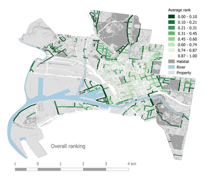
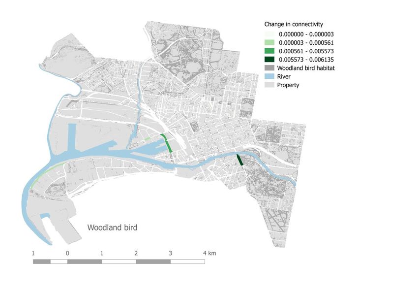
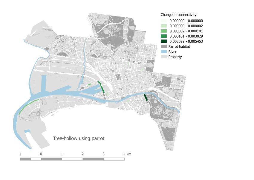
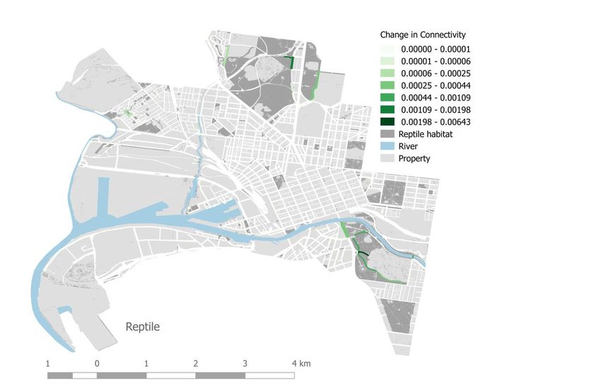
Activity 2 – Identifying priority road segments for connectivity action
Roads form major barriers to movement for many species, especially smaller flying
organisms (such as insects, Muñoz et al., 2015) and terrestrial animals such as
reptiles and amphibians (Forman et al, 2003; Taylor & Goldingay, 2010; Rytwinski &
Fahrig, 2012). Street-lighting along major roads can also impact nocturnal species
(Bliss-Ketchum et al., 2016). Because a large proportion of council owned and
managed land occurs along roads, mitigating the barrier effect of roads may be one of
the most effective ways that the City of Melbourne can improve ecological connectivity
across the municipality. By ranking the contribution of each road segment to landscape
connectivity we can help the City of Melbourne prioritise where to target actions
focused on improving urban biodiversity. To do this, we removed each road segment
one at a time and re-calculated the connectivity index, while keeping the habitat area
and distance threshold constant. The difference between the initial connectivity index
and one calculated after removal of a road segment (i.e. the change in value)
represents the contribution of that road segment to the landscape connectivity. This
process was repeated for all seven animal groups.

The change in the probability of connectedness ranged from 0 to an increase of 0.01
(representing changes in effective mesh size, eff , from 0 Ha to +3.28 Ha). Across
the seven species groups, removing road segments had the biggest effect on
connectivity for the tree-hollow using bat group, followed by the woodland birds,
reptiles, tree-hollow using birds, aquatic insects and amphibians. The insect-pollinator
group showed the smallest changes in connectivity when road segments were
removed. This is probably due to the configuration of existing habitat for that species
group across the City of Melbourne. If significant habitat patches become connected
by removal of a road segment this will cause a larger increase in connectivity. This is
because roads are considered a barrier to movement and therefore prevent nearby
habitat patches from being connected. By quantifying the change in the probability of
connectedness for each road segment we were able to rank the road segments in
order of their overall contribution to landscape connectivity (average rankings in Table
3, Figure 7) and for the seven species groups (Table 4).

We generated maps for each of the species groups which show the road segments
ranked and coloured by their contribution to ecological connectivity (Figure 8). Darker
colours show a greater increase in the connectivity index when that road was removed.
In most cases, removing one road segment made an exceedingly small change to the
connectivity index, or no change at all. This indicates that for many species, removal
of small road barriers alone is not enough to increase landscape-level connectivity:
road-barrier mitigation will need to be combined with the creation of new habitat. It is
also important to remember that this method treated each road segment separately,
whereas a real-life scenario would perhaps mean several road segments would be

 Page 21

changed (or mitigated) at the same time. Despite this, ecological connectivity can be
improved by focussing on mitigating the barrier effect of the road segments detailed in
the following two tables. We highly recommend re-running the connectivity analysis to
quantify the effect of specific roadway interventions (as demonstrated in Linking
Nature in the City – Part One), especially if multiple segments will be targeted together.

Table 3. Top target road segments to improve ecological connectivity in the City of Melbourne. These
roads performed best in an average ranking across the seven different animal groups.

 Segment Average
 Road name
 ID ranking

 1 Government House Drive from Birdwood Avenue 22698 1

 Hotham Street between Hoddle Street & Simpson Street 21910
 2 3
 Old Poplar Road from The Avenue 22407

 3 St Kilda Road between Yarra River & Southbank Boulevard 22087 3.5

 4 Linlithgow Avenue between St Kilda Road and Alexandra Avenue 22696 4

 5 Morell Bridge from Alexandra Avenue 22486 5

 6 Swanston Street between Princes Bridge and Flinders Street 22195 5.5

 Simpson Street between George Street & Hotham Street 21921
 7 Birdwood Avenue between Dallas Brooks Drive & Anzac Avenue 22198 6
 Docklands Drive between Waterfront Way & Pearl River Road 23254

 8 Oak Street between Poplar Road and Manningham Street 22403 6.5

 Simpson Street between Wellington Parade & George Street 22380
 9 Linlithgow Avenue between St Kilda Road & Government House Dr. 22089 7
 The Avenue between Leonard Street & Walker Street 22380

 10 Princes Park Drive between Cemetery Road West & MacPherson St. 22512 7.25

Table 4 (opposite page). Top 10 target roads for improving ecological connectivity in the City of
Melbourne. These are the specific road segments to target for each of the seven animal groups.

 Page 22

Rank Amphibian Reptile Insect pollinator Aquatic insect Tree-hollow bird Bat Woodland bird

 Docklands Government St Kilda Sims St Kilda St Kilda St Kilda
1 23256 22698 22087 21685 22087 22087 22087
 Drive House Drive Road Street Road Road Road

 23311
 Swanston Collins 22452 Harbour Lorimer 22452 Harbour
2 22403 Oak Street 22388 The Avenue 22195 23308 22168
 Street Street 22835 Esplanade Street 22835 Esplanade
 22956
 22801
 Manningham Old Poplar Hotham Bourke Lorimer Harbour Lorimer
3 22416 22407 21910 22913 22168 22835 22168
 Street Road Street Street Street Esplanade Street
 23293

 22696 Linlithgow The St Kilda Docklands Whiteman Lloyd
4 22380 The Avenue 22392 22087 23254 22562 21672
 22089 Avenue Avenue Road Drive Street Street

 Poplar Princes Swanston Lloyd Barry Docklands
5 22932 Cade Way 22404 22512 22195 21672 20476 23254
 Road Park Drive Street Street Street Drive

 Princes
 Princes Park Morell 21921 Simpson Whiteman Drummond Whiteman
6 22512 22486 22512 Park 22562 20542 22562
 Drive Bridge 21949 Street Street Street Street
 Drive

 Birdwood Kensington Salmon Barry Swanston Barry
17 22321 Story Street 22198 21843 22159 20476 20484 20476
 Avenue Road Street Street Street Street

 Queens
 The Dryburgh Batman’s Docklands Batman’s
8 21789 22397 Park Street 21162 22184 Bridge 22802 23254 22802
 Crescent Street Hill Drive Drive Hill Drive
 Street

 Galada Princes 22380 The Queens Drummond Drummond
9 22938 22512 22186 20542 20542
 Avenue Park Drive 22388 Avenue Bridge Street Street

 St Kilda Lloyd La Trobe La Trobe
10 21303 Arden Street 22087 22334 Park Drive 21672 22549 22549
 Road Street Street Street

 Page 23

Figure 7. City of Melbourne road segments coloured by their overall impact on ecological connectivity.
The darker the green colour, the greater the benefit of removing or reducing the barrier effect of that
road segment.

 Page 24

Figure 8. These maps show City of Melbourne road segments coloured by their impact on ecological
connectivity as calculated for the amphibian and reptile groups. The darker the green colour, the greater
the benefit of removing or reducing the barrier effect of that road segment.

 Page 25

Figure 8 (continued). These maps show City of Melbourne road segments coloured by their impact on
ecological connectivity as calculated for the insect pollinator and aquatic insect groups. The darker the
green colour, the greater the benefit of removing or reducing the barrier effect of that road segment.

 Page 26

Figure 8 (continued). These maps show City of Melbourne road segments coloured by their impact on
ecological connectivity as calculated for the tree-hollow using bird and bat groups. The darker the green
colour, the greater the benefit of removing or reducing the barrier effect of that road segment.

 Page 27

Figure 8 (continued). These maps show City of Melbourne road segments coloured by their impact on
ecological connectivity as calculated for the woodland bird group. The darker the green colour, the
greater the benefit of removing or reducing the barrier effect of that road segment.

 Page 28

3. Recommendations

In addition to this report we are providing the raw result files (spreadsheets) from the
sensitivity testing and road-ranking exercise, along with a collection of shape files that
can be loaded into the City of Melbourne’s in-house GIS program, CoMPass. These
shape files can be overlayed on the road segment network to identify where
opportunities for connectivity-improvement overlap with planned capital works.
Visualising roads in this way will make it easier for planning combined capital works
and targeted improvements for specific species groups.

Choosing input parameters
As highlighted in Linking Nature in the City – Part One, when estimating ecological
connectivity there are many assumptions made about how to define what is “habitat”,
how to define what is a “barrier” and how to decide on a distance threshold. The results
from our investigation into the sensitivity of the connectivity index used here indicate
that reducing the uncertainty of these assumptions is important. Where ambiguity
exists in the parameterisation of the distance threshold and the definition of a road
barrier, it is best to calculate the index for the upper and lower limits of each. This
allows the uncertainty in the connectivity index to be quantified for the target species.

Choosing the inputs for a target species involves the following steps:
 1. Identify what resources/habitat the animal needs to survive.
 • Consult with a species expert where possible, but if this is not feasible
 then check the existing ecological literature. Where data on a given
 species are unavailable, look for analogous species (e.g. in a similar
 taxonomic group or ecological niche). Habitat might include specific
 types of vegetation, or abiotic features such as water or cavities.
 • Identify where these resources are within the City, combine the spatial
 information together.
 • This input is likely to be the least uncertain in terms of its species-specific
 definition. However, it is important to be aware of any limitations in the
 availability of spatial data for some resources (e.g. nesting sites, or
 specific plant species) when interpreting the connectivity results.
 2. Identify potential barriers to movement for this species
 • Consult with a species expert where possible, but if this is not feasible
 then check the existing literature. Where data on the specific species are
 unavailable, look for information on species that are similar in behaviour.
 • Consider barriers might include buildings, rivers, rail and tram ways,
 large open spaces, impervious surfaces as well as roads. Some species
 might be able to traverse roads below a certain width, others might only
 cross at night.

 Page 29

• Identify which of these categories could be barriers and combine the
 spatial information for all types of barrier.
 • If there is uncertainty in what features might be considered a barrier to
 this species, it is best to use the most conservative estimate.
 3. Decide what threshold to use to determine whether habitat patches are
 connected*
 • Consult with a species expert where possible, but if this is not feasible then
 check the existing literature. Where data on the specific species are
 unavailable, look for information on species that are similar in size or
 method of movement.
 • The best estimate of movement ability for this application is gap-crossing
 distance. Failing that, min/mean/maximum dispersal distance is a good
 measure. This information can also be obtained from models of dispersal
 probability and home-range size.
 • Where there is uncertainty in the dispersal ability of the target species,
 calculate the connectivity index for the highest and lowest values in the
 range. This will quantify uncertainty and provide two maps which can be
 used to understand the spatial arrangement of connected areas.

*NOTE The distance threshold is used to determine if habitat patches are part of the
same connected area if the patches are not also separated by a barrier.

Based on the connectivity maps generated during the distance sensitivity analysis we
can also identify some key areas where the City of Melbourne might want to consider
creating additional habitat to improve connectivity for each of the seven species
groups. These recommendations were determined by comparing the maps in Figure
4, focussing on places where patches remained unconnected. The suggested actions
detailed below are certain to make a positive impact on ecological connectivity for the
group in question.

Amphibians (e.g. spotted marsh frog Limnodynastes tasmaniensis)
Since amphibians are one of the least mobile species groups, focussing on connecting
habitat patches within parks will help boost connectivity. Concentrating on the areas
within Royal Park and the riparian habitat along the upper Moonee Ponds Creek will
help facilitated amphibian connectivity. The estuarine Yarra River forms a major barrier
for this group, so efforts to improve connectivity will need to take place separately
north and south of the river.

Reptiles (e.g. eastern blue-tongued lizard Tiliqua scincoides)
Similar to amphibians, the suitable habitat patches for reptiles in Royal Park could be
connected, particularly by managing the edges of roads, railway and tram lines that
cross the park. There is also potential in the residential suburb of Kensington to link
up patches of reptile habitat with the Stock Route and surrounding reserves/gardens.

 Page 30

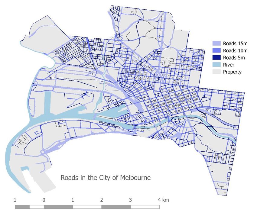
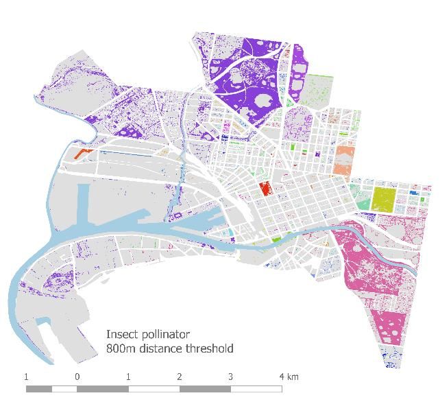
Insect pollinators (e.g. blue-banded bee Amegilla chlorocyanea)
Connectivity can be improved for insect pollinators by concentrating on the creation of
smaller habitat patches between parks, particularly in the suburbs of North Melbourne,
Carlton and East Melbourne. These could be along streets, helping to bridge gaps
between larger, contiguous habitat areas found in parks and gardens.

Aquatic insects (e.g. blue skimmer dragonfly Orthetrum caledonicum)
Improving the abundance and structural diversity of riparian habitat along the Moonee
Ponds Creek and Yarra River will help to increase ecological connectivity for aquatic
insects, which are otherwise well connected within individual parks like Royal Park
and Kings Domain.

Tree-hollow using bird (e.g. red-rumped parrot Psephotus haematonotus)
Ecological connectivity for tree-hollow using birds is already high, the main way to
improve this is to focus on ways to lessen the effect of wide roads, which are the main
barriers to connectedness for this group.

Tree-hollow using bat (e.g. Gould’s wattled bat Chalinolobus gouldii)
Ecological connectivity for tree-hollow using bats is already high, the main way to
improve this is to focus on ways to lessen the effect of wide roads, which are the main
barriers to connectedness for this group, particularly around South Bank.

Woodland bird (e.g. superb fairywren Malurus cyaneus)
Ecological connectivity for woodland birds is already high, the main way to improve
this is to focus on ways to lessen the effect of wide roads, especially around South
Bank and Fishermans Bend.

Mitigating the barrier effect of roads
The City of Melbourne has a relatively high level of habitat available to animal species,
however, there are many barriers to movement across the City that reduce the
landscape-level connectivity. The most extensive of these are the road and rail
networks, although the concentration of buildings in the CBD will also present a major
barrier to many species. Roads form a large proportion of the land owned and
managed by the City of Melbourne, meaning that targeting roadways may be the most
effective way for the City to improve connectivity.

For species which can move relatively easily (birds, bats and larger flying insects), the
wider busier roads (>15 m wide, Figure 9) form the greatest barriers to movement.
These include Flemington Road, Westgate Freeway, Footscray Road, Dynon Road,
St Kilda Road and Royal Parade. Many of these roads pass between or next to major
parks which contain the largest patches of contiguous habitat in the City. Intermediate

 Page 31

sized roads (between 5 and 10 m wide, Figure 9) contribute the most to habitat
fragmentation in more residential areas where habitat availability is high, but patch
sizes are smaller (areas like North Melbourne, Carlton and East Melbourne). These
areas often contain many smaller green spaces which could act as “stepping-stones”
between the larger parks but are prevented from contributing to connectivity because
of the road network. Finally, narrower roads (

Figure 9. The City of Melbourne road and rail network, narrower roads darker, wider roads lighter in
colour. The road grids around the CBD, Carlton, Fitzroy and North Melbourne create fragmentation of
smaller habitat patches which limits the ability of these small patches to be used as stepping-stones
between the larger parks.

 Page 33

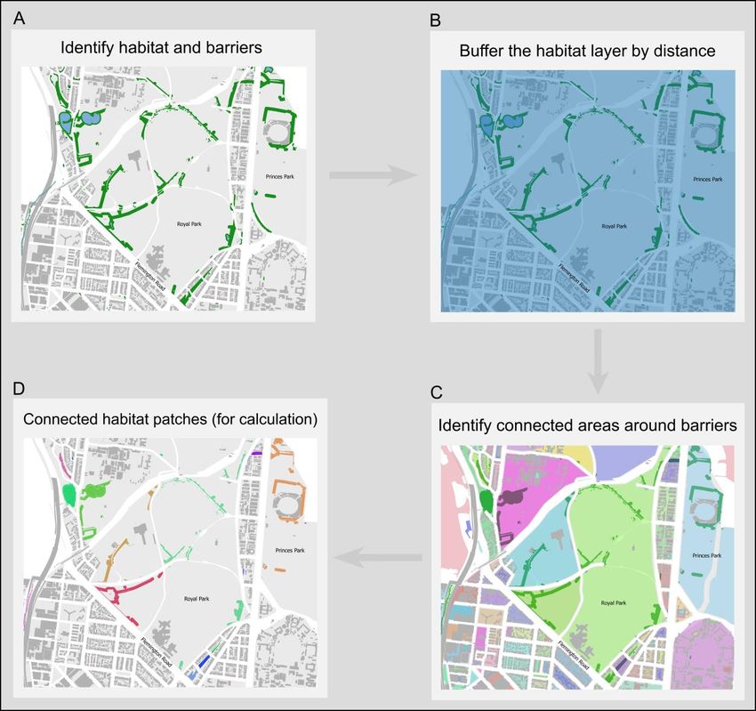
4. Detailed methodology

Glossary of terms

Barrier - a landscape feature which complete impedes movement of an animal.
Depending on the target species in question, roads, railways, tramways and buildings
are all considered movement barriers. In some species open expanses of ground or
large water bodies would also be considered barriers.

Connectivity index – in Linking Nature in the City – Part One we use effective mesh
size ( eff ) as a measure of ecological connectivity. This is a measure of area (Ha)
where increasing the landscape connectivity leads to an increase in connected area.
We converted this to a “probability of connectedness”, scaled between 0 and 1, where
1 would be a completely connected landscape.

Distance threshold – the distance (in metres) beyond which patches of habitat are no
longer considered connected. Usually based on knowledge about the general
dispersal or movement ability of the target species.

Habitat – a collection of different land-use types that can support a species through
the provision of resources such as food, water, nesting sites, shelter or cover. The
definition of habitat changes depending on the species being considered. For
calculation of the connectivity index habitat is

Dispersal capability – ability of the target species to move around the landscape. Can
also be considered the ability of an organism to cross gaps in preferred habitat. This
is usually derived from the results of published research into the home range or daily
movements of the species in question (or related organisms), or by consulting with
species experts.

Calculation of the Connectivity Index
The connectivity index used here (also called the effective mesh size, eff ) can be
calculated using the following equation:

 1
 eff = ∑ 2 
 
 =1

Where = the number of groups of connected patches, = the total area of the
landscape and 2 = size of each of the groups of patches (where = 1, 2, 3, … )
(Spanowicz & Jaeger, 2019). Figure 10 (reproduced from Linking Nature in the City –
Part 1) shows a schematic of how the effective mesh size calculation works. In this
report, we also converted the connectivity index (a measure of area) into a “probability

 Page 34

of connectedness” (scaled between 0 and 1) by dividing the connectivity index or eff
by the total area of habitat. This is analogous to Jaeger’s “degree of coherence”,
defined as “the probability that two animals placed in different areas somewhere in the
region of investigation might find each other” (Jaeger, 2000).

Steps for calculating the connectivity index:
 Part A
 1. Define what land-use types are considered to be habitat for the target species.
 Combine all the different spatial polygons into one spatial layer (Figures 10.A
 & 11.A).
 2. Define what land-use types are considered to be barriers to movement of the
 target species. Combine all the different spatial polygons into one spatial layer.
 3. Remove any habitat patches that currently intersect with the barrier layer. *
 4. Buffer the habitat layer using a fixed distance buffer, with the buffer value set
 to HALF the appropriate threshold distance for the target species (Figures 10.B
 & 11.B). Save the buffered habitat layer as a new spatial layer.
 5. Take the buffered layer and overlay the barrier layer. Remove all areas from
 the buffered habitat layer that lie under the barrier layer. This creates what is
 called a “fragmentation geometry” (Figure 11.C).
 6. Use the fragmentation geometry and the habitat layer to identify which patches
 of habitat are part of the same “connected areas” (Figure 10.C). Classify the
 habitat patched according to which connected area they are part of (i.e. give
 them an ID, Figure 11.D).
 Part B
 7. Determine the total area of the habitat patches within each connected area
 (Figure 10.D). Calculate the 2 of each connected area.
 8. Use the equation for effective mesh size (above) to calculate the Connectivity
 Index in Ha (Figure 10.D).
 9. If needed, calculate the “probability of connectedness” by dividing the
 Connectivity Index value by the Total area of habitat.

* Need to decide how habitat that lies within or on barriers (e.g. road medians) is
treated. This is a complicated issue and depends on how you have defined a “barrier”.

 Page 35

Figure 10. Worked example calculation with diagram. In this example, the landscape contains four
patches of habitat (A). Buffering these habitat patches by a fixed distance determines which are
connected (B). In this example, the two red patches are part of the same connected area. The area of
each individual patch is then calculated (C). These values are used to calculate the connectivity index,
or effective mesh size (D). Note that the two patches that make up the red connected area are summed
together.

 Page 36

Figure 11. Example GIS visualisation of the processing steps required to find the area of connected
habitat available.

When implementing the above workflow in R 3.6.0 the following packages and
functions were used:

Package sf (Pebesma, 2018)
Functions from the sf package were used to prepare the spatial data layers for
analysis (reading, writing and cleaning data). The st_buffer, st_union,
st_intersects, st_area functions were used to identify which habitat patches
were connected and calculate the habitat areas.

Package tidyverse (Wickham, 2017)
Various functions, (especially group_by) from the tidyverse package were used
to identify and remove unwanted road segments and to calculate the average
ranking of roads by their contribution to connectivity.

 Page 37

5. References

Software
R Core Team (2019). R: A language and environment for statistical computing. R Foundation
for Statistical Computing, Vienna, Austria. URL https://www.R-project.org/.

Pebesma, E., 2018. Simple Features for R: Standardized Support for Spatial Vector Data. The
R Journal 10 (1), 439-446, https://doi.org/10.32614/RJ-2018-009

Hadley Wickham (2017). tidyverse: Easily Install and Load the 'Tidyverse'. R package
version 1.2.1. https://CRAN.R-project.org/package=tidyverse

Publications
Baker-Gabb, D., & Hurley, V. G. (2011). National Recovery Plan for the Regent Parrot
 (eastern subspecies) Polytelis anthopeplus monarchoides (p. 29). Department of
 Sustainability and Environment, Melbourne.

Berven, K. A., & Grudzien, T. A. (1990). Dispersal in the wood frog (Rana sylvatica ):
 implications for genetic population structure. Evolution, 44(8), 2047–2056.
 https://doi.org/10.1111/j.1558-5646.1990.tb04310.x

Bliss-Ketchum, L. L., de Rivera, C. E., Turner, B. C., & Weisbaum, D. M. (2016). The effect
 of artificial light on wildlife use of a passage structure. Biological Conservation, 199,
 25–28. https://doi.org/10.1016/j.biocon.2016.04.025

Davis, R. A., Lohr, C. A., & Dale Roberts, J. (2019). Frog survival and population viability in
 an agricultural landscape with a drying climate. Population Ecology, 61(1), 102–112.
 https://doi.org/10.1002/1438-390X.1001

Dolný, A., Harabiš, F., & Mižičová, H. (2014). Home Range, Movement, and Distribution
 Patterns of the Threatened Dragonfly Sympetrum depressiusculum (Odonata:
 Libellulidae): A Thousand Times Greater Territory to Protect? PLoS ONE, 9(7),
 e100408. https://doi.org/10.1371/journal.pone.0100408

Richard T. T. Forman, Daniel Sperling, John A Bissonette, Anthony P Clevenger, Carol D
 Cutshall, Virginia H Dale, Lenore Fahrig, Robert France, Charles R Goldman, Kevin
 Heanue, Julia A Jones, Frederick J Swanson, Thomas Turrentine, and Thomas C
 Winter (2002) Road Ecology: Science and Solutions Washington, DC: Island Press,
 2002.

Garrard, G. E., McCarthy, M. A., Vesk, P. A., Radford, J. Q., & Bennett, A. F. (2012). A
 predictive model of avian natal dispersal distance provides prior information for
 investigating response to landscape change: Prior information on avian dispersal
 distance. Journal of Animal Ecology, 81(1), 14–23. https://doi.org/10.1111/j.1365-
 2656.2011.01891.x
Haddad, N. M. (1999). Corridor and distance effects on interpatch movements: a landscape
 experiment with butterflies. Ecological Applications, 9(2), 612–622.
 https://doi.org/10.1890/1051-0761(1999)009[0612:CADEOI]2.0.CO;2

 Page 38

Harrisson, K. A., Pavlova, A., Amos, J. N., Takeuchi, N., Lill, A., Radford, J. Q., & Sunnucks,
 P. (2013). Disrupted fine-scale population processes in fragmented landscapes
 despite large-scale genetic connectivity for a widespread and common cooperative
 breeder: the superb fairy-wren ( Malurus cyaneus ). Journal of Animal Ecology, 82(2),
 322–333. https://doi.org/10.1111/1365-2656.12007

Heard, G. W., Scroggie, M. P., & Malone, B. S. (2012). Classical metapopulation theory as a
 useful paradigm for the conservation of an endangered amphibian. Biological
 Conservation, 148(1), 156–166. https://doi.org/10.1016/j.biocon.2012.01.018

Kirk H, Threlfall C, Soanes K, Ramalho C, Parris K, Amati M, Bekessy SA, Mata L. (2018)
 Linking nature in the city: A framework for improving ecological connectivity across
 the City of Melbourne. Report prepared for the City of Melbourne Urban Sustainability
 Branch.

Koenig, J., Shine, R., & Shea, G. (2001). The ecology of an Australian reptile icon: how do
 blue-tongued lizards (Tiliqua scincoides) survive in suburbia? Wildlife Research,
 28(3), 214. https://doi.org/10.1071/WR00068

Lees, A. C., & Peres, C. A. (2009). Gap-crossing movements predict species occupancy in
 Amazonian forest fragments. Oikos, 118(2), 280–290. https://doi.org/10.1111/j.1600-
 0706.2008.16842.x

Lowry, H., & Lill, A. (2007). Ecological factors facilitating city-dwelling in red-rumped parrots.
 Wildlife Research, 34(8), 624. https://doi.org/10.1071/WR07025

Lumsden, L. F., Bennett, A. F., & Silins, J. E. (2002). Location of roosts of the lesser long-
 eared bat Nyctophilus geoffroyi and Gould’s wattled bat Chalinolobus gouldii in a
 fragmented landscape in south-eastern Australia. Biological Conservation, 106(2),
 237–249. https://doi.org/10.1016/S0006-3207(01)00250-6

McFarland, D. (1991). The Biology of the Ground Parrot, Pezoporus wallicus, in
 Queensland. I. Microhabitat Use, Activity Cycle and Diet. Wildlife Research, 18(2),
 169. https://doi.org/10.1071/WR9910169

Muñoz, P. T., Torres, F. P., & Megías, A. G. (2015). Effects of roads on insects: a review.
 Biodiversity and Conservation, 24(3), 659–682. https://doi.org/10.1007/s10531-014-
 0831-2

Rytwinski, T., & Fahrig, L. (2012). Do species life history traits explain population responses
 to roads? A meta-analysis. Biological Conservation, 147(1), 87–98.
 https://doi.org/10.1016/j.biocon.2011.11.023

Schultz, C. B. (1998). Dispersal Behavior and Its Implications for Reserve Design in a Rare
 Oregon Butterfly. Conservation Biology, 12(2), 9.

 Page 39

Southwood, T. R. E. (1962). Migration of terrestrial arthropods in relation to habitat.
 Biological Reviews, 37(2), 171–211. https://doi.org/10.1111/j.1469-
 185X.1962.tb01609.x
Taylor, B. D., & Goldingay, R. L. (2010). Roads and wildlife: impacts, mitigation and
 implications for wildlife management in Australia. Wildlife Research, 37(4), 320.
 https://doi.org/10.1071/WR09171

Threlfall, C. G., Law, B., & Banks, P. B. (2013). The urban matrix and artificial light restricts
 the nightly ranging behaviour of Gould’s long-eared bat ( Nyctophilus gouldi ):
 Ranging Behaviour of an Urban Bat. Austral Ecology, 38(8), 921–930.
 https://doi.org/10.1111/aec.12034

Valdez, J. W., Stockwell, M. P., Klop-Toker, K., Clulow, S., Clulow, J., & Mahony, M. J.
 (2015). Factors driving the distribution of an endangered amphibian toward an
 industrial landscape in Australia. Biological Conservation, 191, 520–528.
 https://doi.org/10.1016/j.biocon.2015.08.010

 Page 40