Long-term observations from Antarctica demonstrate that mismatched scales of fisheries management and predator-prey interaction lead to erroneous ...
←
→
Page content transcription
If your browser does not render page correctly, please read the page content below
www.nature.com/scientificreports

            OPEN           Long-term observations from
                           Antarctica demonstrate that
                           mismatched scales of fisheries
                           management and predator-prey
                           interaction lead to erroneous
                           conclusions about precaution
                                                      *
                           George M. Watters           , Jefferson T. Hinke          & Christian S. Reiss

                           Low catch limits for forage species are often considered to be precautionary measures that can help
                           conserve marine predators. Difficulties measuring the impacts of fisheries removals on dependent
                           predators maintain this perspective, but consideration of the spatio-temporal scales over which forage
                           species, their predators, and fisheries interact can aid assessment of whether low catch limits are as
                           precautionary as presumed. Antarctic krill are targeted by the largest fishery in the Southern Ocean and
                           are key forage for numerous predators. Current krill removals are considered precautionary and have
                           not been previously observed to affect krill-dependent predators, like penguins. Using a hierarchical
                           model and 30+ years of monitoring data, we show that expected penguin performance was reduced
                           when local harvest rates of krill were ≥0.1, and this effect was similar in magnitude to that of poor
                           environmental conditions. With continued climate warming and high local harvest rates, future
                           observations of penguin performance are predicted to be below the long-term mean with a probability
                           of 0.77. Catch limits that are considered precautionary for forage species simply because the limit is a
                           small proportion of the species’ standing biomass may not be precautionary for their predators.

                           To conserve large fishes, seabirds, and marine mammals, many stakeholders advocate precautionary management
                           of fisheries that target forage species (e.g., krill, anchovies, and sardines). One strategy to conserve predators is
                           to reserve some proportion of their prey1, perhaps by establishing a low catch limit for the fisheries that target
                           the forage populations or stocks2. However, fishing activities may concentrate where target species are profitably
                           caught, potentially increasing local harvest rates above intended levels3. If management fails to prevent concen-
                           trated fishing where dependent predators forage, these predators may be impacted despite a low overall catch
                           limit. From an ecosystem perspective, the level of precaution implied by a low catch limit may be better-assessed
                           relative to the time and space scales over which forage species, their predators, and fisheries interact.
                               Assessing whether catch limits are precautionary from an ecosystem perspective is challenging because the
                           impacts of forage-fish fisheries on predators are difficult to measure4–6. This difficulty arises because predators
                           respond to many drivers, including environmental conditions and food-web interactions that are modulated by
                           competition and responses to the availability of alternative prey. Reducing uncertainty to draw unambiguous
                           inference about fisheries impacts on predators requires data that disentangle the effects of fishing from those of
                           the environment and match the temporal and spatial scales of predator life histories, predator-prey interactions,
                           and fishery catches. Data of this nature may not be available at the broad scale of the forage stock, but may be so
                           on smaller scales. Experimental approaches to estimate the effects of fishing are possible7, but such experiments
                           are rare and can be controversial8. An alternative to experimentation is to leverage long-term observational data
                           that capture natural and anthropogenic variations in the focal system. Such long-term studies in locations where

                           Antarctic Ecosystem Research Division, Southwest Fisheries Science Center, National Marine Fisheries Service, National
                           Oceanic and Atmospheric Administration, La Jolla, California, 92037, USA. *email: George.Watters@noaa.gov

Scientific Reports |   (2020) 10:2314 | https://doi.org/10.1038/s41598-020-59223-9                                                             1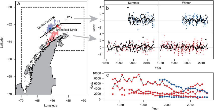
www.nature.com/scientificreports/ www.nature.com/scientificreports
the foraging ranges of predators overlap in time and space with locally intense fishing operations are also rare, but
the observations provided by these studies may include contrasts that are sufficient to improve inference about
the impacts of forage-fish fisheries on dependent predators.
The Antarctic marine ecosystem provides a useful case study for assessing whether a catch limit established at
a regional scale is precautionary given locally high harvest rates. Around the Antarctic Peninsula (AP), Antarctic
krill (Euphausia superba) are the target of the largest fishery in the Southern Ocean9 and a key forage species for
fishes, seabirds, and marine mammals10. The current catch limit for krill in the entire southwest Atlantic sector of
the Southern Ocean is 620,000 tons3. This catch limit is spatially divided across four statistical subareas (48.1, 48.2,
48.3 and 48.4; defined by the Commission for the Conservation of Antarctic Marine Living Resources) to reduce
the risks of negative impacts on krill-dependent predators in the region. The catch limit in Subarea 48.1, which
surrounds the AP, is 155,000 tons, representing 1 Mt) had the smallest effect on
penguin performance (Fig. 2) and had the lowest probability (0.7) that expected performance was reduced from
the best case (Table 1). The probability that a marginal increase in LKB reduced expected penguin performance
below the long-term mean performance was ≤0.04 (Table 1). The insensitivity of penguin performance to varia-
tion in LKB corroborates previous failures to parameterize a functional response3,18,19 and seems consistent with
view that krill biomass in the AP is generally sufficient to support penguin production27.
Warm temperatures (ONI > −0.5 °C) and high LHR (≥0.1) decreased penguin performance, and the
effects of these two factors were similar (Fig. 2). The probabilities that the marginal effects of intermediate ONI
(−0.5 °C < ONI < 0.5 °C) and high LHR caused expected performance to be less than that of the best case were
≥0.93 (Table 1). The probabilities that these marginal effects caused expected penguin performance to be less
than the long-term mean were ≥0.64 (Table 1). In contrast to the best case, we defined the “worst case” as condi-
tions with intermediate ONI, high LKB, and high LHR. Relative to the best case, the worst case caused expected
penguin performance to be below the long-term mean with a probability of 0.99 (Table 1). We have little doubt
that our study populations responded to both the environment and fishing.
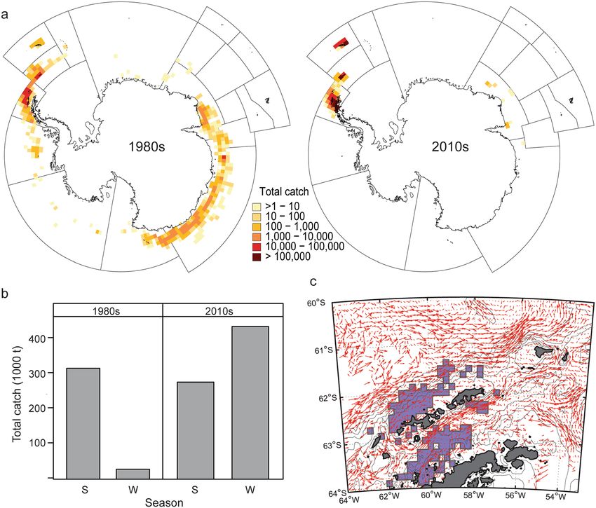
Recent increases in the spatial and temporal concentration of krill catches9,28 provide a plausible mechanism
by which the fishery has affected penguins. During the development of the krill fishery, catches contracted from
a circumpolar distribution to local hotspots near the AP, the South Orkney Islands, and South Georgia (Fig. 3a,
adapted from29). In our Bransfield Strait and Drake Passage strata, annual catches taken prior to 2010 averaged
about 34,000 t/yr30, and LHRs ranged from 0 to 0.01. From 2010 through 2016, catches averaged about 121,000 t/
yr30, and season-specific LHRs ranged from 0 to 0.32, with rates ≥0.1 occurring 20% of the time in the Bransfield
Strait and 10% of the time in the Drake Passage (Supplementary Data S12). For reference, the target harvest rate
used to establish precautionary catch limits for the Antarctic krill fishery is 0.0933. All instances when the LHR
exceeded 0.1 occurred during winter. Winter catches in the AP region have increased over time and now exceed
the total catch taken during summer (Fig. 3b).
Scientific Reports | (2020) 10:2314 | https://doi.org/10.1038/s41598-020-59223-9 2www.nature.com/scientificreports/ www.nature.com/scientificreports
Figure 1. Study area, standardized indices, and trends in penguin abundance. (a) Study area, noting Cape
Shirreff (blue dot), Copacabana (red dot), and Subarea 48.1 (dashed line); the thick black line separates the
Bransfield Strait and Drake Passage strata, and, within these strata, areas of penguin and fishery overlap (adapted
from26 and made available under the Creative Commons CC0 public domain dedication) are respectively
colored light red and light blue. (b) Standardized indices of penguin performance during summer and winter at
Cape Shirreff (blue) and Copacabana (red), acoustic survey (solid black circles) and imputed (open black circles)
estimates of local krill biomass, and the Oceanic Niño Index (thin black line) and Southern Annular Mode
(thick black line). (c) Population trends for Adélie (circles), chinstrap (diamonds) and gentoo (squares) penguins
(colors as in a) (data prior to 2005 replotted from20). Adapted with permission from Springer Nature: Springer-
Verlag Oecologia Divergent responses of Pygoscelis penguins reveal a common environmental driver, J.T. Hinke,
K. Salwicka, S.G. Trivelpiece, G.M. Watters, and W.Z. Trivelpiece, © Springer-Verlag 2007.
Figure 2. Expected performance of penguins attributable to the marginal effects of the Oceanic Niño Index
(ONI), local krill biomass (LKB) and local harvest rate (LHR) relative to the “best case”. The best case is
ONI ≤ −0.5 °C; LKB ≤ 1 Mt; and LHR ≤ 0.01. The “worst case” is −0.5 °C < ONI < 0.5 °C; LKB > 1 Mt; and
LHR ≥ 0.1. The median, interquartile range, and range of the posterior expectations are indicated by each
boxplot. Reference lines respectively indicate the median expected performance in the best case (dashed line)
and the long-term mean performance.
Increased catches taken at smaller spatial scales during winter have increased the frequency of poor penguin
performance and could reduce future recruitment. If the future is represented by our worst case (Fig. 2), the pos-
terior predictive distributions from our model indicate that any performance index, including recruitment, would
be less than its long-term mean with a probability of 0.77 (Table 1). An increased probability of poor recruitment
raises the risk of population declines, as has been shown for Adélie penguins31. Although penguins may compen-
sate so that their performance is not reduced after the birds are “challenged”, e.g.32, the population-level conse-
quences of reductions in performance indices other than recruitment (e.g., longer foraging trips, lower adult mass
at lay) are not always clear4,5. Given the consequences of poor recruitment and the uncertain impacts from other
Scientific Reports | (2020) 10:2314 | https://doi.org/10.1038/s41598-020-59223-9 3www.nature.com/scientificreports/ www.nature.com/scientificreports
Best Long-term
case −0.5 °C < ONI < 0.5 °C ONI ≥ 0.5 °C mean
Best case 0.04 (0.37)
−0.5 °C < ONI < 0.5 °C 1.00 0.88 (0.58)
ONI ≥ 0.5 °C 0.99 0.53 (0.50)
LKB > 1 Mt 0.70 0.02 0.13 0.01 (0.41)
0.01 < LHR < 0.10 0.75 0.17 0.31 0.33 (0.44)
LHR ≥ 0.1 0.93 0.40 0.61 0.64 (0.54)
Worst case 0.99 0.99 (0.77)
Table 1. Posterior and posterior predictive probabilities that expected performance given the effects indicated
in the left-most column are less than the expected performance given effects or conditions indicated in the
column headings. Posterior predictive probabilities are indicated in parentheses. ONI is the Oceanic Niño
Index, LKB is local krill biomass, and LHR is local harvest rate. In the “best case” ONI ≤ −0.5 °C; LKB ≤ 1 Mt;
and LHR ≤ 0.01. In the “worst case” −0.5 °C < ONI < 0.5 °C; LKB > 1 Mt; and LHR ≥ 0.1.
Figure 3. Mechanisms by which krill fishing has impacted penguins. (a) Catches (t) contracted from a
circumpolar distribution of low catches in the 1980s to higher catches concentrated in the southwest Atlantic
sector of the Southern Ocean since 2010. Adapted, with permission from the Secretariat of the Commission for
the Conservation of Antarctic Marine Living Resources, from29. (b) Catches, by decade, taken from Statistical
Subarea 48.1 (see Fig. 1) during summer (S) and winter (W). (c) Area of overlap (adapted from26 and made
available under the Creative Commons CC0 public domain dedication) between foraging predators and the
fishery krill fishery (shaded polygons) with surface water movements from drifters (red arrows). Large arrows
indicate stronger flows.
reductions in performance, the fine-scale concentration of catches taken under the umbrella of a regional catch
limit established for an entire year does not seem to be as precautionary as presumed.
Climate change has implications for whether management of the krill fishery will be precautionary in the
future. It is reasonable to expect that warmer conditions will become more frequent in the AP33, increasing the
probability of negative impacts on penguins. Even as climate changes in the AP, we expect there will be “good”
Scientific Reports | (2020) 10:2314 | https://doi.org/10.1038/s41598-020-59223-9 4www.nature.com/scientificreports/ www.nature.com/scientificreports
years in which penguin performance is above average. However, because fishery effects on penguin performance
are of similar magnitude to those of poor environmental conditions (Fig. 2), performance during good years
might nevertheless be reduced if management of the krill fishery unintentionally facilitates high LHRs. If the
current management strategy for krill is maintained over the long term, future years like our worst case scenario
seem more likely given the propensity of the krill fishery to target hotspots, the regional scale of the current catch
limit, and the expectation of continued warming. As noted previously, such conditions are predicted to cause
expected penguin performance to fall below its long-term mean with a probability of 0.77 (Table 1).
The recovery of cetacean populations in the Southern Ocean also has implications for whether management
of the krill fishery will be precautionary. In the southwest Atlantic sector of the Southern Ocean, humpback whale
populations have increased rapidly in the last 30 years, and recent abundance estimates suggest these populations
have recovered to levels approximating their pre-exploitation abundances34. On one hand, such recoveries of large
cetaceans in the Southern Ocean may reduce the “krill surplus”35 that followed industrial whaling. Alternatively,
increased krill consumption by whales may fertilize surface waters and increase the productivity of the ecosys-
tem36,37. Cetaceans forage in areas where our study penguins overlap with the krill fishery38, and the effects of
increasing cetacean populations on the structure and function of the ecosystem may affect penguin performance.
Determining whether future management of the krill fishery is precautionary will benefit from consideration of
such ecosystem perspectives by effectively improving estimates of LKB, and thus LHR.
At least two caveats might bias the LHRs computed here. First, our estimates of LHR might be biased high
if the catches were taken from areas in which the throughput of krill was sufficient to replenish local standing
stocks. However, penguins foraging from our monitoring sites overlap with the krill fishery in areas where surface
currents are relatively weak (Fig. 3c, with panel c adapted from26), and habitat models suggest that chinstrap pen-
guins throughout the AP and South Orkney Islands forage in slow moving water39. Second, the ongoing recovery
of whale populations in the Southern Ocean has the potential to impact penguin populations21. If consumption by
baleen whales had indeed reduced the standing stocks of krill in areas where our study penguins overlapped with
the krill fishery, the LHRs calculated here might be biased low. However, even in this case, the estimated pattern
of decreased penguin performance with increased LHR would remain.
Variations in the environment (here indexed by the ONI) and LKB may affect penguin performance in myr-
iad, complex ways. For example, precipitation has been negatively correlated with both chick survival and fledg-
ling mass40,41. Also, when the standing stock of krill is large, small krill are proportionally more abundant22, and,
when small krill are more abundant, chinstrap penguins take longer foraging trips20. The literature provides many
examples of links between environmental conditions, the characteristics of the prey field, and penguin perfor-
mance. Our emphasis here has not been to further elucidate or validate such links. Rather we attempt to place
the indirect effects of krill fishing in context with these other drivers of penguin performance, which offers a new
perspective.
In areas with reduced throughput, fishing may reduce the availably of krill to penguins via absolute reductions
in krill biomass (exploitative competition) or from changing the structure of krill swarms or their distribution
in the water column (interference competition). Distinguishing these alternatives is difficult in general5 and not
possible here. However, concentrated krill fishing in hotspots is associated with sequential reductions in catch per
unit fishing effort followed by vessel movements to new areas28. Furthermore, though high LHRs caused reduc-
tions in penguin performance (Fig. 2), these occasions were not coincident with biomasses that were also low
enough to reduce penguin performance. In combination, our results thus suggest that interference competition
has occurred around the AP, whereby krill fishing was sufficient to change the structure or distribution of krill
swarms such that both penguins and the fishery itself were impacted. This hypothesis is testable. In our opinion,
it is now feasible, using modern acoustic equipment, to estimate what might have been caught without actually
bringing krill on deck. Thus, an experiment could be designed in which an acoustic survey is first conducted to
estimate LKB; “normal” fishing activities are then conducted, except with open nets so that krill can escape, until
more than 10% of the local biomass might have been caught; and penguin performance is simultaneously mon-
itored. It might be useful to compare results from this treatment to those from a reference area in which fishing
was conducted with nets that are closed.
Our results demonstrate that it is generally inadvisable to presume the catch limit for a forage species is pre-
cautionary simply because the limit is a small proportion of the species’ standing biomass at a regional scale. The
dynamic nature of forage species and the fisheries that target them1,4,42,43 means that catch limits applied at coarse
spatio-temporal scales can result in unintentionally high LHRs that impact predators. Our integrated, long-term
monitoring data demonstrate that this has occurred in the Antarctic krill fishery because the implementation of a
presumed precautionary approach did not manage the behavior of the fishery to find and exploit hotspots. When
the time and space scales of catch limits are coarser than the scales of predator-prey interactions, it is difficult to
achieve ecosystem objectives that include predator conservation6. Impacts on predators can likely be mitigated
by spatial and temporal allocation schemes that broadly distribute catches to account for predator-prey-fishery
interactions44,45. Failing this, a precautionary approach to conserve predators foraging in fishing hotspots would
be to decrease regional catch limits below the levels that are considered precautionary from a single-species
perspective.
Methods
Strata. We defined two geographical strata to spatially match season-specific penguin foraging locations with
estimates of LKB and LHR. These strata were based on areas where foraging penguins and krill fishing overlap26
and on the availability of krill biomass estimates from research-vessel surveys22,23. We defined the strata as the
Drake Passage, combining the western and Elephant Island survey strata of the U.S. AMLR Program22, and the
Bransfield Strait (Fig. 1a, adapted from26).
Scientific Reports | (2020) 10:2314 | https://doi.org/10.1038/s41598-020-59223-9 5www.nature.com/scientificreports/ www.nature.com/scientificreports
Predictors. We quantified variation in LKB using long-term acoustic survey data22,23 from the AP col-
lected following standard protocols46,47. We computed the density (g/m2) of krill for each nautical mile of survey
effort, computed the average density within each stratum, and multiplied those averages by the area of each
stratum. Summer surveys were conducted in January and February; winter surveys were conducted in August
and September. When more than one survey was conducted in a single season (e.g., January and February of the
same year), we averaged the biomass estimates from those surveys. Summer surveys cover the period 1996-2011
(Fig. 1b). Winter surveys are available for 2012, 2014, and 2015 (Fig. 1b).
We computed LHRs by matching catches with temporally and spatially coincident estimates of LKB. Catch
data were provided by the Secretariat for the Commission for the Conservation of Antarctic Marine Living
Resources. We summed these data by season and stratum and computed LHR as local catch/LKB.
We used two climate indices to characterize seasonal variation in environmental conditions (Fig. 1b). We
averaged monthly values of the Southern Annular Mode (SAM48) for winter (April-September) and summer
(October-March) indices. We also computed seasonal averages of the Oceanic Niño Index (ONI)49. We assigned
summer averages of the SAM and ONI to the second calendar year of the split year in each austral summer (e.g.,
the average value for October 2004 - March 2005 was assigned to 2005).
We categorized all four predictors. When the SAM is in a positive (negative) phase, westerly winds are stronger
and shifted towards the pole50, with a resulting increase (decrease) in air temperature51 and precipitation52 on the
western side of the AP. We thus categorized the SAM according to its sign. The ONI defines La Niña and El Niño
events when sea-surface temperature anomalies near the equator are respectively ≤−0.5 °C and ≥0.5 °C. Such
events interact with the SAM to affect primary production and krill near the Antarctic Peninsula15, so we binned
the ONI into three categories (ONI ≤ −0.5 °C; −0.5 °C < ONI < 0.5 °C; and ONI ≥ 0.5 °C) using these two tem-
perature thresholds. Estimates of LKB are imprecise22 and may be biased by a variety of factors, including the
throughput of krill through our strata53. Nevertheless, the surveys distinguish periods of relative krill scarcity
and abundance. Acoustic estimates of LKB ranged in magnitude from 104 to 107 t. In contrast, krill catches taken
within our strata were reported by fishing vessels, treated as known, and ranged in magnitude from ≤103 to 105 t.
Given differences in the uncertainties and magnitudes of local biomasses and catches, we categorized estimates
of LKB using a threshold of 1 × 10⁶ t (1 Mt) and of LHR using thresholds of 0.01 and 0.1. The threshold for LKB
evenly splits the observed orders of magnitude in krill biomass, and that for LHR provides three categories of
fishing that reflect low harvest rates, harvest rates up to that used to set catch limits for krill (0.093), and fishing
above that level.
Response – penguin performance. We used monitoring parameters based on observations collected dur-
ing 1982-2016 at two field camps in the South Shetland Islands to quantify variations in penguin performance.
Unless otherwise noted, methods of data collection have been described previously20,54. All methods were per-
formed in accordance with relevant guidelines and regulations, including field methods that were reviewed and
approved by the University of California San Diego Institutional Animal Care and Use Committee (ID: S05480)
and authorized under U.S. Antarctic Conservation Act permits (ID: ACA 2017-012). Some parameters reflect
winter conditions (mean clutch-initiation date, mean female and male masses at lay, mean egg density, and rela-
tive cohort strength; Fig. 1b). Other parameters reflect conditions during the summer breeding season (fledgling
mass, foraging-trip duration, and post-hatch breeding success; Fig. 1b). In all but one case, these parameters
integrate over days to months. Relative cohort strength integrates over a period ≥1 year, but we assumed that
most of its variation is attributable to survival during the first few months of independence20. We transformed
mean clutch-initiation dates and foraging-trip durations so that larger values would indicate better performance.
The former parameter was transformed to days prior to 31 December (earlier clutch initiations indicate better
performance); the latter was transformed to hourswww.nature.com/scientificreports/ www.nature.com/scientificreports
not be less than catch i ) and an upper limit equal to 100 Mt (so LKBij would be less than twice the estimate of krill
biomass used to manage the krill fishery46). We used results from the acoustic surveys to specify prior distribu-
tions for the imputation model.
(
Kij ~ U 0.1k ij , 10k ij )
(
φ ~ U 0.1sij , 10sij ) (2)
k ij is the mean ln LKB computed from survey observations in stratum i given sign j of the SAM, and sij is the stand-
( )
ard deviation of these log-biomass estimates. We predicted missing estimates of LKB LKBij⁎ from Eq. (1) using
the sign of the SAM for summers when acoustic surveys were not conducted. Missing estimates of LHR, denoted
as LHR⁎, were estimated from LKBij⁎.
LHR ij⁎ = catch i /LKBij⁎ (3)
We did not impute missing values for winter.
In the second component of our model, we treated all indices of penguin performance as exchangeable obser-
vations, and modeled performance (P) as a function of categorized ONI (o), LKB (b), and LHR (h).
p ~ N (P , σ 2 )
P = α + β1o1 + β 2o2 + β 3b + β4h1 + β5h 2 (4)
2
P is the expected performance, and σ is the residual variance in performance. α quantifies mean performance
across the set of predictor categories, and the parameters β1, β 2, β 3, β4, and β5 quantify the degree to which
each predictor causes expected performance to deviate from this mean. We specified prior distributions that limit
inference to the study populations and the predictor bins considered here.
α ~ N (0, 1.0 × 10⁴ )
β1 ~ N (0, 1.0 × 10⁴ )
β 2 ~ N (0, 1.0 × 10⁴ )
β 3 ~ N (0, 1.0 × 10⁴ )
β4 ~ N (0, 1.0 × 10⁴ )
β5 ~ N (0, 1.0 × 10⁴ ) (5)
We specified a half-Cauchy prior distribution for the standard deviation of penguin performance and a uni-
form hyperprior for the scale parameter (ω) of the half-Cauchy56,57.
σ ~ half − Cauchy(ω 2) (6)
ω ~ U(0, 2) (7)
⁎ ⁎
We specified a design matrix with sum-to-zero contrasts that carries uncertainties in LKB and LHR through
the model.
−1 if ONI ≤ − 0.5
o1 =
0 if ONI ≥ 0.5
1
if − 0.5 < ONI < 0.5
−1 if ONI ≤ − 0.5
o2 =
0 if − 0.5 < ONI < 0.5
1
if ONI ≥ 0.5
b= {−1
1
if LKB or LKB ⁎ ≤ 1 Mt
if LKB or LKB ⁎ > 1 Mt
−1 if LHR or LHR⁎ ≤ 0.01
h1 =
0 if LHR or LHR⁎ ≥ 0.1
1
if 0.01 < LHR or LHR⁎ < 0.1
−1 if LHR or LHR⁎ ≤ 0.01
h2 =
0 if 0.01 < LHR or LHR⁎ < 0.1
1
if LHR or LHR⁎ ≥ 0.1 (8)
We used JAGS , via R , to sample from the posterior distributions of the model parameters. After 250,000
58 59
adaptive and 500,000 burn-in iterations, we sampled 5,000 points (retaining values from every 25th iteration dur-
ing a further 125,000 iterations) from the posterior distributions characterized by three Monte Carlo chains initi-
ated at different points in the parameter space. We evaluated our model with a variety of diagnostics. Diagnostics,
Scientific Reports | (2020) 10:2314 | https://doi.org/10.1038/s41598-020-59223-9 7www.nature.com/scientificreports/ www.nature.com/scientificreports
data files, and the code needed to replicate our analysis are provided as Supplemental Information. Three R pack-
ages are needed to run our code: rjags60, coda61, and ggmcmc62.
Data availability
All model code and data used to conduct this study are included in Supplementary Information files of this
published article.
Received: 19 June 2019; Accepted: 22 January 2020;
Published: xx xx xxxx
References
1. Pikitch, E. et al. Little fish, big impact: managing a crucial link in ocean food webs. (Lenfest Ocean Program, Washington, D.C.
2012).
2. Constable, A. J., de la Mare, W. K., Agnew, D. J., Everson, I. & Miller, D. Managing fisheries to conserve the Antarctic marine
ecosystem: practical implementation of the Convention on the Conservation of Antarctic Marine Living Resources (CCAMLR).
ICES J. Mar. Sci. 57, 778–791 (2000).
3. Hill, S. L. et al. Is current management of the Antarctic krill fishery in the Atlantic sector of the Southern Ocean precautionary?
CCAMLR Sci. 23, 31–51 (2016).
4. Hilborn, R. et al. When does fishing forage species affect their predators? Fish. Res. 191, 211–221 (2017).
5. Sydeman, W. J. et al. Best practices for assessing forage fish fisheries-seabird resource competition. Fish. Res. 194, 209–221 (2017).
6. Hunsicker, M. E. et al. Functional responses and scaling in predator-prey interactions of marine fishes: contemporary issues and
emerging concepts. Ecol. Lett. 14, 1288–1299 (2011).
7. Pichegru, L., Gremillet, D., Crawford, R. J. M. & Ryan, P. G. Marine no-take zone rapidly benefits endangered penguin. Biol. Lett. 6,
498–501 (2010).
8. Cherry, M. African penguins put researchers in a flap. Nature 514, 283 (2014).
9. Nicol, S., Foster, J. & Kawaguchi, S. The fishery for Antarctic krill - recent developments. Fish. Fish. 13, 30–40 (2012).
10. Everson, I. Marine Interactions in Antarctic Ecology, volume 2. (ed. Laws, R. M.) 463–490 (Academic Press 1984).
11. Polito, M. J., Lynch, H. J., Naveen, R. & Emslie, S. D. Stable isotopes reveal regional heterogeneity in the pre-breeding distribution
and diets of sympatrically breeding Pygoscelis spp. penguins. Mar. Ecol. Prog. Ser. 421, 265–277 (2011).
12. Volkman, N. J., Presler, P. & Trivelpiece, W. Diets of Pygoscelid penguins at King George Island, Antarctica. Condor 82, 373–378
(1980).
13. Miller, A. K. & Trivelpiece, W. Z. Cycles of Euphausia superba recruitment evident in the diet of Pygoscelid penguins and net trawls
in the South Shetland Islands, Antarctica. Polar Biol. 30, 1615–1623 (2007).
14. Loeb, V. et al. Effects of sea-ice extent and krill or salp dominance on the Antarctic foodweb. Nature 387, 897–900 (1997).
15. Saba, G. K. et al. Winter and spring controls on the summer food web of the coastal West Antarctic Peninsula. Nat. Commun. 5,
4318, https://doi.org/10.1038/ncomms5318 (2014).
16. Atkinson, A. et al. Krill (Euphausia superba) distribution contracts southward during rapid regional warming. Nat. Clim. Change 9,
142–147 (2019).
17. Flores, H. et al. Impact of climate change on Antarctic krill. Mar. Ecol. Prog. Ser. 458, 1–19 (2012).
18. Scientific Committee for the Conservation of Antarctic Marine Living Resources. Report of the twenty-second meeting of the
Scientific Committee. CCAMLR, Hobart; https://www.ccamlr.org/en/meetings/27 (2003).
19. Hewitt, R. P. et al. Options for allocating the precautionary catch limit of krill among small-scale management units in the Scotia Sea.
CCAMLR Sci. 11, 81–97 (2004).
20. Hinke, J. T., Salwicka, K., Trivelpiece, S. G., Watters, G. M. & Trivelpiece, W. Z. Divergent responses of Pygoscelis penguins reveal a
common environmental driver. Oecologia 153, 845–855 (2007).
21. Trivelpiece, W. Z. et al. Variability in krill biomass links harvesting and climate warming to penguin populations in Antarctica. Proc.
Natl. Acad. Sci. USA 108, 7625–7628 (2011).
22. Reiss, C. S., Cossio, A. M., Loeb, V. & Demer, D. A. Variations in the biomass of Antarctic krill (Euphausia superba) around the
South Shetland Islands, 1996-2006. ICES J. Mar. Sci. 65, 497–508 (2008).
23. Reiss, C. S. et al. Overwinter habitat selection by Antarctic krill under varying sea-ice conditions: implications for top predators and
fishery management. Mar. Ecol. Prog. Ser. 568, 1–16 (2017).
24. Croxall, J. P., Trathan, P. N. & Murphy, E. J. Environmental change and Antarctic seabird populations. Science 297, 1510–1514
(2002).
25. Loeb, V. J. & Santora, J. A. Climate variability and spatiotemporal dynamics of five Southern Ocean krill species. Prog. Oceanogr. 134,
93–122 (2015).
26. Hinke, J. T. et al. Identifying risk: concurrent overlap of the Antarctic krill fishery with krill-dependent predators in the Scotia Sea.
PLoS One 12, e0170132, https://doi.org/10.1371/journal.pone.0170132 (2017).
27. Sailley, S. F. et al. Carbon fluxes and pelagic ecosystem dynamics near two western Antarctic Peninsula Adélie penguin colonies: an
inverse model approach. Mar. Ecol. Prog. Ser. 492, 253–272 (2013).
28. Santa Cruz, F., Ernst, B., Arata, J. A. & Parada, C. Spatial and temporal dynamics of the Antarctic krill fishery in fishing hotspots in
the Bransfield Strait and South Shetland Islands. Fish. Res. 208, 157–166 (2018).
29. Commission for the Conservation of Antarctic Marine Living Resources. Krill Fishery Report 2018. (CCAMLR, Hobart); https://
www.ccamlr.org/en/document/publications/krill-fishery-report-2018. (2018).
30. Commission for the Conservation of Antarctic Marine Living Resources. Statistical Bulletin, vol. 30. (CCAMLR, Hobart); https://
www.ccamlr.org/en/publications/statistical-bulletin (2018).
31. Hinke, J. T., Trivelpiece, S. G. & Trivelpiece, W. Z. Variable vital rates and the risk of population declines in Adélie penguins from the
Antarctic Peninsula region. Ecosphere 8, e01666, https://doi.org/10.1002/ecs2.1666 (2017).
32. Ballard, G. et al. Responding to climate change: Adélie Penguins confront astronomical and ocean boundaries. Ecology 91,
2056–2069 (2010).
33. Clarke, A. et al. Climate change and the marine ecosystem of the western Antarctic Peninsula. Philos. T. R. Soc. Lon. B. 362, 149–166
(2006).
34. Zerbini, A. N. et al. Assessing the recovery of an Antarctic predator from historical exploitation. R. Soc. Open Sci. 6, 190368, https://
doi.org/10.1098/rsos.190368 (2019).
35. Laws, R. Seals and whales of the Southern Ocean. Philos. Trans. R. Soc. Lond. 279, 81–96 (1977).
36. Roman, J. & McCarthy, J. J. The whale pump: marine mammals enhance primary productivity in a coastal basin. PLoS One 5, 10,
https://doi.org/10.1371/journal.pone.0013255 (2010).
37. Nicol, S. et al. Southern Ocean iron fertilization by baleen whales and Antarctic krill. Fish. Fish. 11, 203–209 (2010).
38. Weinstein, B. G., Double, M., Gales, N., Johnston, D. W. & Friedlander, A. S. Identifying overlap between humpback whale foraging
grounds and the Antarctic krill fishery. Biol. Cons. 210, 184–191 (2017).
Scientific Reports | (2020) 10:2314 | https://doi.org/10.1038/s41598-020-59223-9 8www.nature.com/scientificreports/ www.nature.com/scientificreports
39. Trathan, P. N. et al. Managing fishery development in sensitive ecosystems: Identifying penguin habitat use to direct management in
Antarctica. Ecosphere 9, e02392, https://doi.org/10.1002/ecs2.2392 (2018).
40. Chapman, E. W., Hofmann, E. E., Patterson, D. L., Ribic, C. A. & Fraser, W. R. Marine and terrestrial factors affecting Adélie penguin
Pygoscelis adeliae chick growth and recruitment off the western Antarctic Peninsula. Mar. Ecol. Prog. Ser. 436, 273–289 (2011).
41. Cimino, M. A., Fraser, W. R., Patterson-Fraser, D. L., Saba, V. S. & Oliver, M. J. Large-scale climate and local weather drive
interannual variability in Adélie penguin chick fledging mass. Mar. Ecol. Prog. Ser. 513, 253–268 (2014).
42. Atkinson, A. et al. Sardine cycles, krill declines, and locust plagues: revisiting ‘wasp-waist’ food webs. Trends Ecol. Evol. 29, 309–316
(2014).
43. Cury, P. et al. Small pelagics in upwelling systems: patterns of interaction and structural changes in “wasp-waist” ecosystems. ICES
J. Mar. Sci. 57, 603–618 (2000).
44. Plagányi, E. E. & Butterworth, D. S. The Scotia Sea krill fishery and its possible impacts on dependent predators: modeling localized
depletion of prey. Ecol. App. 22, 748–761 (2012).
45. Watters, G. M., Hill, S. H., Hinke, J. T., Matthews, J. & Reid, K. Decision-making for ecosystem-based management: evaluating
options for a krill fishery with an ecosystem dynamics model. Ecol. App. 23, 710–725 (2013).
46. Scientific Committee for the Conservation of Antarctic Marine Living Resources. Report of the twenty-ninth meeting of the
Scientific Committee. CCAMLR, Hobart; https://www.ccamlr.org/en/meetings/27 (2010).
47. Calise, L. & Skaret, G. Sensitivity investigation of the SDBWA Antarctic krill target strength model to fatness, material contrasts and
orientation. CCAMLR Sci. 18, 97–122 (2011).
48. U.S. National Weather Service. https://www.cpc.ncep.noaa.gov/products/precip/CWlink/daily_ao_index/aao/monthly.aao.index.
b79.current.ascii
49. U.S. National Weather Service. https://origin.cpc.ncep.noaa.gov/products/analysis_monitoring/ensostuff/ONI_v4.shtml
50. Thompson, D. W. J. & Wallace, J. M. Annular modes in the extratropical circulation. Part I: month-to-month variability. J. Clim. 13,
1000–1016 (2000).
51. Marshall, G. J., Orr, A., van Lipzig, N. P. M. & King, J. C. The impact of a changing Southern Hemisphere Annular Mode on
Antarctic Peninsula summer temperatures. J. Clim. 19, 5388–5404 (2006).
52. Marshall, G. J., Thompson, D. W. J. & van den Broeke, M. R. The signature of Southern Hemisphere atmospheric circulation patterns
in Antarctic precipitation. Geophys. Res. Lett. 44, 11580–11589 (2017).
53. Hofmann, E. E. & Murphy, E. J. Advection, krill, and Antarctic marine ecosystems. Antarct. Sci. 16, 487–499 (2004).
54. Commission for the Conservation of Antarctic Marine Living Resources. CCAMLR ecosystem monitoring program standard
methods. (CCAMLR, Hobart, 2014).
55. Hoyt, D. F. Practical methods of estimating volume and fresh weight of bird eggs. Auk 96, 73–77 (1979).
56. Gelman, A. Prior distributions for variance parameters in hierarchical models (comment on article by Browne and Draper).
Bayesian Anal. 1, 515–534 (2006).
57. Polson, N. G. & Scott, J. G. On the half-cauchy prior for a global scale parameter. Bayesian Anal. 7, 887–902 (2002).
58. Plummer, M. JAGS: A Program for Analysis of Bayesian Graphical Models Using Gibbs Sampling. Proceedings of the 3rd
International Workshop on Distributed Statistical Computing. March 20-22, Vienna, Austria. ISSN 1609-395×(2003).
59. R Core Team. R: a language and environment for statistical computing. https://www.R-project.org (2018).
60. Plummer, M., Stukalov, A. & Denwood, M. Bayesian graphical models using MCMC. http://mcmc-jags.sourceforge.net (2016).
61. Plummer, M., Best, N., Cowles, K. & Vines, K. CODA: convergence diagnosis and output analysis for MCMC. R News 6, 7–11 (2006).
62. Fernández-i-Marín, X. ggmcmc: analysis of MCMC samples and Bayesian inference. J. Stat. Softw. 70, 1–20 (2016).
Acknowledgements
This research was conducted as part of the U.S. Antarctic Marine Living Resources Program of the National
Oceanic and Atmospheric Administration (NOAA). We thank the numerous field teams that collected data on
krill and penguins over the last 3 + decades. We thank A.M. Cossio for synthesis of acoustic survey data, W.Z. and
S.G. Trivelpiece for a life-long commitment to the study of penguins in Antarctica, D.J. Krause and M. Mangel for
comments on an early version of this manuscript, and G. Cutter for being a naturalist. Borrego Springs, California
provided the desert heat required to cook this manuscript. Finally, the Editor and two referees provided extensive
suggestions to improve our paper.
Author contributions
G.M.W. designed the study; G.M.W., J.T.H. and C.S.R. conducted research, analyzed data, and wrote the paper.
Competing interests
The authors declare no competing interests.
Additional information
Supplementary information is available for this paper at https://doi.org/10.1038/s41598-020-59223-9.
Correspondence and requests for materials should be addressed to G.M.W.
Reprints and permissions information is available at www.nature.com/reprints.
Publisher’s note Springer Nature remains neutral with regard to jurisdictional claims in published maps and
institutional affiliations.
Open Access This article is licensed under a Creative Commons Attribution 4.0 International
License, which permits use, sharing, adaptation, distribution and reproduction in any medium or
format, as long as you give appropriate credit to the original author(s) and the source, provide a link to the Cre-
ative Commons license, and indicate if changes were made. The images or other third party material in this
article are included in the article’s Creative Commons license, unless indicated otherwise in a credit line to the
material. If material is not included in the article’s Creative Commons license and your intended use is not per-
mitted by statutory regulation or exceeds the permitted use, you will need to obtain permission directly from the
copyright holder. To view a copy of this license, visit http://creativecommons.org/licenses/by/4.0/.
© The Author(s) 2020
Scientific Reports | (2020) 10:2314 | https://doi.org/10.1038/s41598-020-59223-9 9You can also read