Long-term surveys of age structure in 13 ungulate and one ostrich species in the Serengeti, 1926-2018 - Nature
←
→
Page content transcription
If your browser does not render page correctly, please read the page content below
www.nature.com/scientificdata

               OPEN           Long-term surveys of age structure
Data Descriptor               in 13 ungulate and one ostrich
                              species in the Serengeti, 1926–2018
                              Pierre Rogy    ✉ & Anthony R. E. Sinclair

                              The Serengeti ecosystem spans an extensive network of protected areas in Tanzania, eastern Africa,
                              and a UNESCO Wold Heritage Site. It is home to some of the largest animal migrations on the planet.
                              Here, we describe a dataset consisting of the sample counts of three age classes (infant, juvenile and
                              adult) of 13 ungulate and one ostrich species. Sample counts were tallied visually from the ground, or,
                              in some instances, aerial photographs, during a period extending from 1926 to 2018. Observed animals
                              were assigned to age classes based on specific criteria for each species. For nine of the 14 species of
                              this dataset, the number of sampling years is over 30. This resulted in a total of 533 different records
                              of count across age classes. By computing age-class ratios, these data can be used to measure long-
                              term recruitment success at different ages of the tallied species. In particular, the temporal extent of
                              these data allows comparison of patterns to other long-term processes, such as the El Niño-Southern
                              Oscillation (ENSO).

                              Background & Summary
                              Located in Tanzania, the Serengeti ecosystem (34–36 °E, 1–4 °S) has been a protected area since the 1920s, and
                              is home to a great diversity of ungulate species. Over the past 150 years, this ecosystem has experienced several
                              major perturbations that have affected the ecological dynamics of many these ungulate species. First, a panzootic
                              due to the exotic rinderpest virus affected most ungulates, in particular wildebeest and buffalo, whose popula-
                              tions were decimated in the 1890s1. A very slow recovery followed, until the virus disappeared in 1963. After this
                              local extirpation of the virus, these two species experienced exponential increase until numbers levelled out in
                              19772. Second, intensive hunting has been an important threat to the ungulate populations. For example, in the
                              mid-1800s, elephants were abundant in the ecosystem, but, by 1890, all had been killed for the ivory trade3. In
                              1951, when the Serengeti National Park was gazetted, greater conservation protection from poaching allowed
                              recovery in all protected species4. In fact, it is only after 1950 that, through immigration of other populations
                              from outside the core area, the elephant population of the Serengeti started a local resurgence, reaching a high
                              point in 19753,5. Following this, a second wave of ivory poaching reduced numbers to 10% of their previous high.
                              In 1988, after the ban on ivory trading, poaching ceased and the elephant population rebounded to its highest
                              density in 20146. Ungulate populations of the ecosystem now face new threats7. Anthropogenic climate change
                              induces acute modifications in precipitation patterns, particularly through variations in the El Niño-Southern
                              Oscillations (ENSO)8. These changes are reflected in increasing fluctuations in vegetation patterns, which will
                              ultimately influence the survival of ungulates9,10.
                                  These examples illustrate that, in order to assess responses to human and environmental pressures, popula-
                              tions need to be monitored over the long run11. In ungulates, such responses have traditionally been measured
                              through changes in reproductive success. This is usually accomplished by recording samples of two age groups
                              of young animals relative to the number of females with which they are associated. In the case of the dataset
                              presented here, the first age group, “infants”, indicates the early survival of young animals (less than six months
                              of age, an unusual term used to make it applicable to both ungulates and ostrich) at the end of the rainy season
                              (March–June). The second age group, “juveniles”, (between nine and 18 months of age, depending on the species)
                              records the survival of young animals through the dry season, the period of food shortage.
                                  This dataset consists of 13 species of ungulates: the African buffalo (Syncerus caffer Sparrman 1779), eland
                              (Taurotragus oryx Pallas 1766), elephant (Loxodonta africana Blumenbach 1797), Grant’s gazelle (Nanger granti

                              Department of Zoology and Biodiversity Research Centre, University of British Columbia, 6270 University Boulevard,
                              Vancouver, British Columbia, V6T 1Z4, Canada. ✉e-mail: pierre.rogy@gmail.com

  Scientific Data |   (2020) 7:359 | https://doi.org/10.1038/s41597-020-00701-0                                                                1
www.nature.com/scientificdata/ www.nature.com/scientificdata
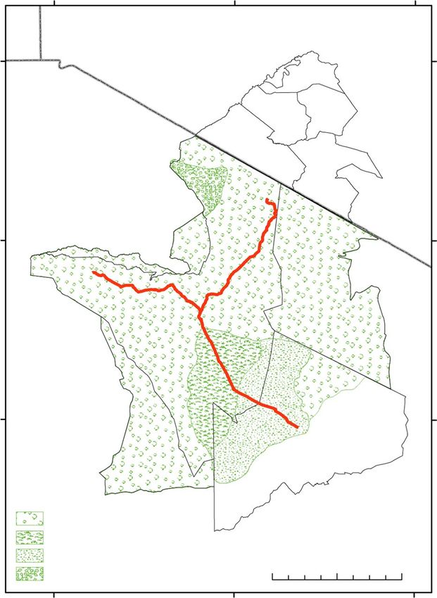
Fig. 1 Ungulate and ostrich sampling transects in the Serengeti ecosystem.
Brooke 1872), Thomson’s gazelle (Eudorcas thomsonii Günther 1884), giraffe (Giraffa camelopardalus tippelskirchi
Brisson 1772), impala (Aepyceros melampus Lichtenstein 1812), Coke’s hartebeest or kongoni (Alcelaphus buse-
laphus Pallas 1766), topi (Damaliscus lunatus Burchell 1824), warthog (Phacochoerus africanus Gmelin 1788),
Defassa waterbuck (Kobus defassa Rüppell 1835), wildebeest (Connochaetes taurinus Burchell 1823), and zebra
(Equus quagga Boddaert 1785). In addition, this dataset includes similar measurements for the ostrich (Struthio
camelus Linnaeus 1758). Samples were obtained by driving along roads and recording the age and sex of animals
out to approximately 100 m, a distance where age classes can still be readily identified. For common species, listed
in Method 1 below, this sampling was conducted once or twice a year at specific times, while, for rarer species,
listed in Method 2 below, observations were ad hoc and all records for the year were summed. A special case of
Method 1 were the very large herds of wildebeest (C. taurinus) and zebra (Eq. quagga), for which subsampling
along transects were needed. Very early samples of African buffalo (Sy. caffer), giraffe (G. camelopardalus) and
wildebeest (C. taurinus) were obtained from aerial photographs (Method 3, explained below). Although they
do not provide a complete census of the populations, these data can be used to estimate rates of reproduction (#
infants/ # adult females) or effective recruitment (# juveniles / # adult females) across the years of sampling.
Methods
There were three methods of sampling the populations. For Methods 1 and 2, records were obtained by driving
along the road transects, and stopping to score the age groups in herds within some 100 m of the road. There
were three road transects, entirely in the administrative boundaries of Serengeti National Park and consistent
every year (1962–2018), with records summed over the three for each data entry. Transect 1 was from Seronera
(34.823°E, 2.428°S) west to Kirawira (34.208°E, 2.151°S; 120 km), Transect 2 from Seronera to Bologonja
(35.173°E, 1.757°S; 115 km), and Transect 3 from Seronera to Olduvai Gorge (35.35°E, 2.993°S; 75 km) (Fig. 1).
The first two transects were in similar savanna ecosystems, and comparison of samples from these two showed
close similarity.
The criteria for age classes in each species are given in Online-only Table 1. The sample was the herd within
view (such as a group of impalas (Ae. melampus) or hartebeests (Al. buselaphus), which occur in discrete groups),
or a subset of it if the herd was very large. One observer, using 8–10 x magnification binoculars, called out the age
category while a recorder entered the records on data sheets. These were later entered digitally.
Two exceptions to this were the immense herds of migrant wildebeest (C. taurinus) and zebra (Eq. quagga).
Because they were numerous and extensive, herds had to be sampled in a systematic way. A vehicle drove through
the herds, stopping every half kilometer, where a 180 degree scan out to 100 m was conducted to count the sample
within view. The transects were from the start to the end of the herd, with some being 30 km long through a single,
continuous herd. Method 3 used aerial pictures of the herds to score age groups. Although the sampling protocol
Scientific Data | (2020) 7:359 | https://doi.org/10.1038/s41597-020-00701-0 2www.nature.com/scientificdata/ www.nature.com/scientificdata
Variable Description Unit
order Linnaean order of species
family Linnaean family of species
genus Linnaean genus of species
specific_epithet Linnaean specific epithet of species
naming_authority Scientific name authorship
common_name Common name of species
year Year of sampling
month Month of sampling
infant Count of infants Individuals
juvenile Count of juveniles Individuals
female Count of adult females Individuals
Count of adult males and females (i.e. when adult males and females
unid_adult Individuals
could not readily be differentiated)
Whether the population is migrant (“M”) or resident (“R”) in the
migrant_resident
ecosystem
Which age classes were recorded for that specific sample:
infants + juveniles + females (“ijf ”), infants + juveniles + all adults
sampling_type
(“ija”), infants + females (“if ”), juveniles + females (“jf ”), infants + all
adults (“ia”), or juveniles + all adults (“ja”)
Whether sampling Method 1 (sampling once or twice a year at specific
sampling_method times), 2 (yearly counts for rare species) or 3 (tallying using aerial
pictures) was used for that specific sample
Table 1. Description of dataset variables.
was different in the three methods (due to different distributions of each species) the same criteria for identifying
age classes was used in all methods. All methods used either systematic or random sampling of the populations.
All species were either migrants, if the species shows seasonal variation in habitat, or residents, if the species
remains in the same area of the park year-round. A notable exception to this is the wildebeest (C. taurinus). In
fact, there were two populations of wildebeest, a large migrant herd and a small resident herd at the far western
end of the ecosystem. These two were sampled separately and scored as either migrant or resident.
Method 1. This method was used in all sampling years for impala (Ae. melampus), Coke’s kongoni (Al. busela-
phus), topi (D. lunatus), warthog (P. africanus), Defassa waterbuck (K. defassa), and zebra (Eq. quagga). Sampling
years 1984–1994 for African buffalo (Sy. caffer), 1965–2012 for giraffe (G. camelopardalus), and 1964–2016 for
wildebeest (C. taurinus).
Populations were sampled once or twice a year at specific times, depending on the availability of different age
classes in the areas near transects. Because ungulates had different birth seasons samples were collected at two
time periods, once in mid-year and once at year-end. Only one time period per year was used for each species.
The early age group, “infants”, was sampled usually near the end of the rainy season (March–June) since many spe-
cies give birth during the rainy season. For some species, there was a second sampling period (August-December)
at the end of the dry season, to measure the survival of juveniles during this period of ecological stress. There are
a few cases where more than two samples were obtained in a single year, so as to track the survival of the whole
cohort throughout a year.
Method 2. This method was used in all sampling years for eland (T. oryx), elephant (L. africana), Grant’s
gazelle (N. granti), ostrich (S. camelus), and waterbuck (K. defassa).
These species were sufficiently scarce that an adequate sample could not be obtained at specific times. For
these, records were scored whenever the species was seen in a sampling period, and then records for all sam-
pling periods of a single given year were summed. A special case was Thomson’s gazelle (Eu. thomsonii), which,
although numerous, was scored only during one short time period (1992–1994) for the months of August and
September.
Method 3. This method was used in sample years 1965–1973 for African buffalo (Sy. caffer), and 1926–1933
for giraffe (G. camelopardalus tippelskirchi), wildebeest (C. taurinus), and zebra (Eq. quagga). The area covered
was in all cases within the Serengeti ecosystem. Buffalo and giraffe were only found in the savanna, while wilde-
beest were sampled when they were on the plains. Flights were made systematically over the area, wildebeest was
sampled using photographs at regular intervals, buffalo and giraffe were sampled when they were encountered.
The third method, applied only in the very early years, used aerial photographs to identify age classes and
females. The same criteria for identifying age classes was used as those for Methods 1 and 2 (Online-only Table 1),
with an emphasis on the shape and size of horns for the wildebeest and African buffalo2, and of the relative sizes of
young giraffe. The early samples in 1926–1933, were obtained from photographs taken by Martin Johnson. These
photos reside in the Martin and Osa Johnson Safari Museum, Chanute, Kansas. Unfortunately, the 1965–1973
photographs of buffalo herds have now all been lost or destroyed.
Scientific Data | (2020) 7:359 | https://doi.org/10.1038/s41597-020-00701-0 3www.nature.com/scientificdata/ www.nature.com/scientificdata
Data Records
The dataset includes 533 different year-month-species measurement, represented as a list of species names and
their count in each age class. As shown in Table 1, the data consist of 15 columns comprising taxonomic informa-
tion, count in each age class, as well as the information on sampling. The data are provided in a .txt file12.
Technical Validation
Sampling of all herds seen along transects was designed to provide an unbiased measurement of recruitment suc-
cess in the populations relative to the number of females. Therefore, males were not part of this sampling program
for most species. This focus on females was important because males of many species separate from the female
herds and become solitary or form bachelor herds. An unbiased sampling of males would therefore require an
unmanageably large sample over the whole ecosystem. However, the sexes of two species, zebra (Eq. quagga) and
warthog (P. africanus), could not be identified with certainty so males and females were recorded together as adults.
In both of these species, males are evenly distributed with the females, so sampling remained relatively unbiased.
This observation is based on a subset of data where the sexes could be distinguished and on published research13.
In addition, although age is continuous, our age categories were discrete. This could induce bias when observed
young are at the border of two age categories. However, the observers used consistent criteria to identify age classes
(Online-only Table 1). In order to reduce the different individual biases that could arise from different observers,
only one (A.R.E. Sinclair) scored the observations before 1997, including the photographs, and four observers con-
ducted the survey between 1997 and 2018. All other observers were thoroughly trained by A.R.E. Sinclair.
Code availability
The code for compiling and generating the dataset is available in the Github repository for the project14.
Received: 16 July 2020; Accepted: 29 September 2020;
Published: xx xx xxxx
References
1. Spinage, C.A. In African Ecology. (ed. Spinage, C.A.) Ch. 22 (Springer, 2012).
2. Sinclair, A. R. E. The African Buffalo. A Study of Resource Limitation of Populations (Chicago Univ. Press, 1977).
3. Dublin, H. T., Sinclair, A. R. E. & McGlade, J. Elephants and Fire as Causes of Multiple Stable States in the Serengeti-Mara
Woodlands. J. of Anim. Ecol. 59(3), 1147–1164 (1990).
4. Sinclair, A. R. E. In Serengeti II: Dynamics, Management and Conservation of an Ecosystem (eds. Sinclair, A. R. E. & Arcese, P.) Ch. 9
(Chicago Univ. Press, 1995).
5. Ahlering, M. A. et al. Identifying source populations and genetic structure for savannah elephants in human‐dominated landscapes
and protected areas in the Kenya‐Tanzania borderlands. PLoS One 7, e52288 (2012).
6. Mduma, S., Musyoki, C., Maliti Kyale, D. et al. Aerial total count of elephants and buffaloes in the Serengeti‐Mara ecosystem. World
Wide Fund for Nature, Nairobi. (2014).
7. Veldhuis, M. P. et al. Cross-boundary human impacts compromise the Serengeti-Mara ecosystem. Science 363(6434), 1424–1428
(2019).
8. Cai, W. et al. Increasing frequency of extreme El Niño events due to greenhouse warming. Nature Clim. Change 4, 111–116 (2014).
9. Sinclair, A. R. E. et al. Asynchronous food web pathways buffer the response of Serengeti predators to El Niño Southern Oscillation.
Ecology 94, 1123–1130 (2013).
10. Sinclair, A. R. E. et al. Serengeti IV: Sustaining biodiversity in a coupled human-natural system (Chicago Univ. Press, 2015).
11. Kiffner, C. et al. Long-term population dynamics in a multi-species assemblage of large herbivores in East Africa. Ecosphere 8(12),
e02027 (2017).
12. Rogy, P. & Sinclair, A. R. E. Long-term surveys of age structure in 13 ungulate and one ostrich species in the Serengeti, 1926–2018.
KNB Data Repository https://doi.org/10.5063/F1VX0DW4 (2020).
13. Klingel, H. The social organization and population ecology of the plains zebra (Equus quagga). Zool. Afr. 4, 249–264 (1969).
14. Rogy, P. Serengeti_data_rescue Github https://github.com/pierrerogy/seregenti_data_rescue (2020).
Acknowledgements
This dataset was compiled under the Living Data Program, an initiative of the Canadian Institute of Ecology
and Evolution (CIEE). Internship funding was provided to P.R. through an NSERC CREATE training program
entitled “Computational Biodiversity Science and Services” (BIOS²). We would like to thank Rene Beyers for
plotting the map in Fig. 1. Two anonymous reviewers, Diane Srivastava, Francesca Fogliata and Nadia Páez
provided useful comments on the manuscript, and Laura Melissa Guzman on the data compilation process. The
Martin and Osa Johnson Safari Museum, Chanute, Kansas kindly provided the early aerial photos. The work was
funded by the Canadian Natural Sciences and Engineering Research Council, the Frankfurt Zoological Society
and the Wildlife Conservation Society of New York.
Author contributions
The data were collected in the research program of A.R.E. Sinclair and colleagues. Photographs of early herds
were scored by A.R.E. Sinclair. He digitised the data, which were then compiled by P. Rogy. Both authors worked
jointly on the data descriptor.
Competing interests
The authors declare no competing interests.
Additional information
Correspondence and requests for materials should be addressed to P.R.
Reprints and permissions information is available at www.nature.com/reprints.
Scientific Data | (2020) 7:359 | https://doi.org/10.1038/s41597-020-00701-0 4www.nature.com/scientificdata/ www.nature.com/scientificdata
Publisher’s note Springer Nature remains neutral with regard to jurisdictional claims in published maps and
institutional affiliations.
Open Access This article is licensed under a Creative Commons Attribution 4.0 International
License, which permits use, sharing, adaptation, distribution and reproduction in any medium or
format, as long as you give appropriate credit to the original author(s) and the source, provide a link to the Cre-
ative Commons license, and indicate if changes were made. The images or other third party material in this
article are included in the article’s Creative Commons license, unless indicated otherwise in a credit line to the
material. If material is not included in the article’s Creative Commons license and your intended use is not per-
mitted by statutory regulation or exceeds the permitted use, you will need to obtain permission directly from the
copyright holder. To view a copy of this license, visit http://creativecommons.org/licenses/by/4.0/.
The Creative Commons Public Domain Dedication waiver http://creativecommons.org/publicdomain/zero/1.0/
applies to the metadata files associated with this article.
© The Author(s) 2020
Scientific Data | (2020) 7:359 | https://doi.org/10.1038/s41597-020-00701-0 5You can also read