Managing uncertainty of expert's assessment in FMEA with the belief divergence measure
←
→
Page content transcription
If your browser does not render page correctly, please read the page content below
www.nature.com/scientificreports
OPEN Managing uncertainty of expert’s
assessment in FMEA with the belief
divergence measure
Yiyi Liu & Yongchuan Tang*
Failure mode and effects analysis (FMEA) is an effective model that identifies the potential risk in
the management process. In FMEA, the priority of the failure mode is determined by the risk priority
number. There is enormous uncertainty and ambiguity in the traditional FMEA because of the
divergence between expert assessments. To address the uncertainty of expert assessments, this work
proposes an improved method based on the belief divergence measure. This method uses the belief
divergence measure to calculate the average divergence of expert assessments, which is regarded
as the reciprocal of the average support of assessments. Then convert the relative support among
different experts into the relative weight of the experts. In this way, we will obtain a result with
higher reliability. Finally, two practical cases are used to verify the feasibility and effectiveness of this
method. The method can be used effectively in practical applications.
Risk assessment and prevention have drawn more and more attention in modern management. Risk represents
the probability of an adverse event which will breach security and pose a threat. Assessments of risk are largely
dependent on an analysis of the uncertainty. Failure mode and effects analysis (FMEA), a risk assessment method
widely used in engineering and m anagement1, was first proposed by the Department of Defense, USA in 19492
and used to solve quality and reliability problems in military products. FMEA has been gradually applied to
all walks of life, including a erospace3, automobile manufacturing4, the medical field5, food safety6, and sup-
plier selection7. The main purpose of FMEA is to identify potential failure modes and assess their causes and
influences8. The core parameter of FMEA is risk priority number (RPN)9, which is the product of three risk
factors, which are the occurrence (O), severity (S), and detection (D) of a failure mode. The failure modes are
ranked according to their RPN, and the failure mode with the highest RPN has the higher priority.
The traditional FMEA model can be roughly described as the following steps. (1) Identifying all failure modes
in the target system. (2) Assessing the risk factors of these failure modes by experts. (3) Calculating the RPN
value of failure modes according to the result of assessments. (4) Ranking the failure modes on the basis of RPN
value. However, in practice, there is a great deal of uncertainty in assessing potential risks in systems with the
traditional FMEA model, often yielding imprecise results. Because it is difficult to reach an agreement on the
assessment of failure mode by different experts10, coupled with the inaccurate cognition of the real problem by
experts, the assessment of risk is inaccurate and u ncertain11. For example, if a very authoritative expert gives an
assessment of a failure mode is (5,6,7) (assuming that his assessment is very close to the truth), the RPN value
is 210. And another expert gives an assessment is (3,1,4). The RPN value is 12. Obviously, due to the second
expert’s subjective opinion or incomplete understanding of the problem, their assessment has great ambiguity
and uncertainty. The average RPN value is 111. It is very different from the real situation. In addition, the tradi-
tional FMEA has some defects12,13. First, the traditional FMEA model ignored the relative importance between
the three risk factors named O, S, and D. Different risk factors should have different weights, so there is no way
to unify the weights of the three risk factors. Second, the traditional FMEA model divides ratings of O, S, and
D into non-linear scales of grades [1, 2, 3, ..., 10]. It will eventually produce many repeated and intermittent
values that will affect the ability of the management personnel to make effective decisions. Third, there are some
subjective assumptions about the assessments of the failure mode by experts. Enough attention should be given
to the weighting of each expert.
For the above problems, some existing studies propose many methods to deal with the uncertainty in risk
assessments by adopting existed theories such as fuzzy sets t heory14,15, Dempster-Shafer evidence t heory16,
evidence reasoning17, prospect theory18, D-number theory19, Z-number t heory20, R-number t heory21, fairness-
oriented consensus approach22, grey relation analysis method23, and best-worst method24. Among them, Liu et al.
School of Big Data and Software Engineering, Chongqing University, Chongqing 401331, China. *
email:
tangyongchuan@cqu.edu.cn
Scientific Reports | (2022) 12:6812 | https://doi.org/10.1038/s41598-022-10828-2 1
Vol.:(0123456789)
www.nature.com/scientificreports/
propose a method combining the fuzzy theory and technique for order preference by similarity to ideal solution
(TOPSIS)25, which achieves the calculation of weights of expert decisions based on similarity. Wang et al. capture
the experts’ diverse assessments on the risk of failure modes and the weights of risk factors by interval two-tuple
linguistic variables and develop a ranking method for failure modes based on the regret theory and T ODIM26.
27
In , the authors use the ambiguity measure(AM) to quantify the degree of uncertainty assessed by each expert
for each risk item. An AM-based weighting method for weighted risk priority number is proposed in28. A FMEA
method based on rough set and interval probability theories is proposed in29, which converts the assessment
values of risk factors into interval numbers, and the interval exponential RPN is proposed to overcome the dis-
continuity problem of traditional RPN values. In30, the authors propose a FMEA method based on Deng entropy
under the Dempster-Shafer evidence theory framework, where the uncertainty of expert assessments is measured
by Deng entropy and converted into the relative weights of experts and weights of risk factors. In addition to
the above studies, some researchers have done some studies based on similarity measure in FMEA . I n31, Zhou
et al. use the Similarity Measure Value Method (SMVM) to model the failure modes and their correlations. This
method gains similarity among assessments based on the concept of medium curve and fuzzy number. Pang et al.
propose a method to weight the experts based on the similarity of their assessments, which is calculated by fuzzy
Euclidean distance32. Furthermore, Jin et al.’s research introduce the Dice similarity and the Jaccard s imilarity33.
However, little research is conducted to improve FMEA from the standpoint of divergence measure, despite the
fact that divergence measure and similarity measure share some characteristics, while Song and Wang use the
form of “1 − D(A, B)” (D(A, B) represents the divergence of evidence) to measure the similarity34. Most previous
researches have improved the FMEA in view of the process of assessment. Those methods are able to effectively
model the experts’ assessments as accurate data and deal with them with some appropriate methods. But for the
data that has been modeled, it is necessary to measure the uncertainty among them by some methods, such as
the divergence measure. Due to the fact that there is little research which combines the divergence measure and
FMEA, the effectiveness of the method that introduces divergence measure into FMEA is necessary to verify.
It’s also the motivation of this paper.
Because of the influence of subjective opinion and historical experience, expert assessments are often inac-
curate. The uncertainty among the assessments by different experts needs to be measured by some appropri-
ate methods. Processing data with imprecise information can be done using the Dempster-Shafer evidence
theory35,36. In Dempster-Shafer evidence theory, how to measure the divergence and conflicts between the
evidence remains an open issue37. There are many uncertainty measurement methods38, such as ambiguity
measure39, total uncertainty m easure40, divergence m easure41, the correlation c oefficient42, and the fractal-based
belief entropy43. Recently, X
iao44 proposed the belief divergence measure (BJS) on the basis of the Jensen-Shannon
divergence measure45. By replacing the probability assignment function with the mass function, BJS is able to
effectively measure the divergence between different pieces of evidence. Therefore, this work propose an expert
assessment uncertainty analysis method based on BJS.
The new method models the belief structure of expert assessment results, calculate the divergence among
BPAS with BJS, and construct the divergence degree matrix. Since the divergence degree and the support degree
of assessments are opposite concepts, the divergence degree of other BPAS to the current BPA is regarded as
the reciprocal of the support degree. This theory is used to convert the average divergence degree into the aver-
age support degree, which is used to represent the weight of experts. By bringing the weight of experts into the
calculation of RPN, a more accurate analysis of expert assessments will be obtained and the risk of the system
will be reduced. Compared with other improved methods, BJS calculates the reliability by combining all the
evidence rather than calculating the credibility of each piece of evidence in isolation, so the results calculated in
this way have higher reliability. In addition, the method considers the relative importance of different experts,
reduces the uncertainty caused by divergence that is produced by the subjectivity of different experts, and is
more in line with the actual situation.
This paper’s contribution is that the new method proposed solutions in view of the traditional FMEA defects,
in this way, provide a new idea to improve the FMEA method. In addition, this paper provides some new theoreti-
cal support for the research combining divergence and FMEA. The rest of this work is organized as follows: in
Preliminaries" section reviews the theoretical basis of this work. In "FMEA method based on belief divergence
measure" section, aiming at FMEA, an expert assessment uncertainty measurement method based on the belief
divergence measure is proposed. Then, an actual case is used to verify the application of this method in "Applica-
tions and discussion" section. Finally, "Conclusion" section summarizes the content of this work.
Preliminaries
Dempster‑Shafer evidence theory. The D-S evidence theory (DST) is a very effective tool to process
the data with uncertainty. From data modeling to uncertainty measurement and data fusion, every step has
useful methods to finish. Research on the DST has made great progress in recent years. Accordingly, the FMEA
method in DST has great advantages. The DST was first proposed by Dempster in 1967 and further developed
by Shafer46,47. DST is a generalization of Bayesian subjective probability theory and also an extension of classi-
cal probability theory. As a mathematical framework for representing uncertainty, DST combines the degree of
belief from independent evidence items. DST is defined as below:
Supposing is a fixed, exhaustive set of mutually exclusive events whose probability of occurrence does not
interfere with each other. is expressed by the following formula:
� = {H1 , H2 , H3 , . . . , Hn } (1)
where is called the frame of discernment, and the set of all subsets of (such as formula (2)) is called the power
set of , which is recorded as 2 .
Scientific Reports | (2022) 12:6812 | https://doi.org/10.1038/s41598-022-10828-2 2
Vol:.(1234567890)
www.nature.com/scientificreports/
2� = {∅, {H1 }, {H2 }, . . . , {Hn }, {H1 , H2 }, {H1 , H2 , . . . , Hn }} (2)
where ∅ is an empty set, and the elements in 2 are called propositions.
The mass function, also known as basic probability assignment (BPA), represents the mapping relationship
between an element in 2 and interval [0,1]. It is defined as follows:
m : 2 → [0, 1] (3)
Mass function also satisfy the condition as follows:
m(∅) = 0, m(A) = 1
(4)
A⊂�
For a focus element A of , its Belief function bel (A) is defined as follows:
Bel(A) = m(B)
(5)
B⊆A
The plausibility function pl (A) of A is defined as follows:
pl(A) = m(B) (6)
A∩B=∅
The bel(A) is the lower bound function of proposition A, and the pl(A) is the upper bound function of
proposition A.
Assuming that m1 and m2 are two BPAS under the frame of discernment , B and C are the focus elements of
m1 and m2, respectively. By using the Dempster’s combination rule, the two groups of BPAS are fused to obtain
a new set of probabilities. Dempster’s combination rule is defined as follows:
1
m(A) = (m1 ⊕ m2 )(A) = m1 (B)m2 (C) (7)
1−k B∩C=A
where k represents the degree of conflict between two evidence bodies, which is called the conflict coefficient,
k is defined as follows:
k= m1 (B)m2 (C) (8)
B∩C=∅
FMEA. FMAE is a management tool for system reliability with a highly structured approach that provides a
set of effective technologies for risk assessment and p revention11,48, and has been widely used in product quality
monitoring, decision-making, other fields. FMEA mainly relies on experts to assess different failure modes so
as to determine the priority of each failure mode. Those failure modes with a high RPN value often get focused
attention to reduce the risk of the system effectively. The calculation of RPN is an important step in FMEA, and
the definition of RPN is as follows:
The RPN consists of the probability of failure occurrence (O), the severity of failure occurrence (S), and the
probability of failure being detected (D). The traditional RPN model multiplies the three risk factors (O, S, and
D) to obtain the RPN value, as shown in formula 9:
RPN = O × S × D (9)
In tradition, the grades of O, S, and D are often divided into 10 levels, in which each level of assessment is
given different explanations. The assessment level for O is shown in Table 1, and the assessment levels for S and
D can be found in49.
Divergence measure. The divergence measure can effectively measure the divergence and conflict between
evidence. The divergence, like the similarity, measures the conflict from a distance perspective, but the diver-
gence and similarity are diametrically opposed concepts.There are many existing divergence measurements,
summarized below.
For two probability distributions A = a1 , a2 , . . . , an and B = b1 , b2 , . . . , bn . The JS divergence measure is
denoted as45:
1
Ai
Bi
JS(A, B) = Ai log 1 1
+ Bi log 1 1 (10)
2 2 Ai + 2 Bi 2 Ai + 2 Bi
i i
The BJS divergence measure was proposed by Xiao based on the JS divergence measure. Supposing that there
are two BPAS, m1 and m2, the BJS divergence measure between them is denoted a s44:
1 m1 + m 2 m1 + m 2
BJS(m1 , m2 ) = S m1 , + S m2 , (11)
2 2 2
where,
Scientific Reports | (2022) 12:6812 | https://doi.org/10.1038/s41598-022-10828-2 3
Vol.:(0123456789)www.nature.com/scientificreports/
Level Possibility of failure Probability range of occurrence
10 Extremely high ≥ 1/2
9 Very high 1/3
8 Slightly high 1/8
7 High 1/20
6 Middle high 1/80
5 Middle 1/400
4 Relatively low 1/2000
3 Low 1/15000
2 Slightly low 1/150000
1 Hardly occurs 1/1500000
Table 1. Classification of failure mode occurrence probability.
m1 (Ai )
S(m1 , m2 ) = m1 (A1 ) log
i
m2 (Ai )
BJS is also defined as the following formula:
m1 + m 2 1 1
BJS(m1 , m2 ) = H( ) − H(m1 ) − H(m2 )
2 2 2
(12)
1
2m1 (Ai )
2m2 (Ai )
= m1 (Ai ) log( )+ m2 (Ai ) log( )
2 m1 (Ai ) + m2 (Ai ) m1 (Ai ) + m2 (Ai )
i i
where, H(mj ) represents Shannon entropy, and H (mj ) is defined as:
H(mj ) = − mj (Ai ) log mj (Ai ) (13)
i
The Reinforced belief divergence measure (RB divergence measure) was proposed by Xiao in 2019. It mainly
measures the divergence among belief functions. For two belief functions in the frame of discernment, m1 and
m2, the RB divergence measure is denoted a s50:
|B(m1 , m1 ) + B(m2 , m2 ) − 2B(m1 , m2 )|
RB(m1 , m2 ) = (14)
2
where
2
2 k k
m1 (Ai )
Ai ∩ Aj
B(m1 , m2 ) = m1 (Ai ) log 1 1
2 m1 (Ai ) + 2 m2 (Aj )
|Aj |
i=1 j=1
k k
(15)
2
2
Ai ∩ Aj
m2 (Ai )
+ m2 (Ai ) log 1 1
2 m1 (Ai ) + 2 m2 (Aj )
|Ai |
i=1 j=1
The divergence measure proposed by Wang et al. between m1 and m2 is denoted a s51:
1 PBlm1 (θi )
D(m1 , m2 ) = PBlm1 (θi ) log 1
2 2 PBlm1 (θi ) + PBlm2 (θi )
θ ⊂�
i
(16)
1 PBlm2 (θi )
+ PBlm2 (θi ) log 1
2 2 PBlm 1 (θi ) + PBlm2 (θi )
θ ⊂� i
Compared with Wang et al. divergence, the BJS represents the divergence directly from the view of entropy
without calculating the pl function. As for RB divergence, most assessments in FMEA are regarded as proposi-
tions with a single element, so the RB divergence will be complex and inefficient in FMEA. The BJS is based on
the JS divergence measure and is the extent of the JS divergence measure. BJS is widely used in belief functions.
When all the hypothesis of belief functions are assigned to a single element, the BBA will transform into prob-
ability. At this time, the BJS will degenerate into JS44.
FMEA method based on belief divergence measure
This work proposed a method for calculating RPN value based on the divergence measure, which uses BJS under
the framework of Dempster-Shafer evidence theory to measure the divergence between evidence. In FMEA,
the expert’s assessment is regarded as a piece of evidence. The divergence between different assessments will be
Scientific Reports | (2022) 12:6812 | https://doi.org/10.1038/s41598-022-10828-2 4
Vol:.(1234567890)www.nature.com/scientificreports/
converted into uncertainty of assessment and relative weight of experts. The specific conversion will be carried
out according to the following process:
Step 1: Identify potential failure modes in the target system based on past experience.
Step 2: The risk factors of these failure modes are assessed by experts, and the assessments are mod-
eled as BPA. Assume that the ith expert’s assessments of a risk factor are modeled as a mass function mi =
(m(1),
m(2), . . . , m(10)), the m(θ) represent that the probability of the expert gives the level as θ . m(θ) satisfy
that 10θ=1 m(θ) = 1.
Step 3: BJS is used to measure the divergence between each expert’s assessment, and the divergence matrix
(DMM) is constructed. The DMM is defined as follows:
BJS11 BJS12 . . . BJS1n
BJS BJS22 . . . BJS2n
DMM = 21 (17)
... ... ... ...
BJSn1 BJSn2 . . . BJSnn
where BJSij represents the divergence between mi and mj . Obviously, the DMM has the following two
characteristics:
1. The values on the main diagonal of DMM are 0, because when the two pieces of evidence are exactly the same,
i.e., m1 = m2, BJS (m1 , m2) = 0, indicating that there is no divergence between the two pieces of evidence,
which also conforms to the definition of BJS.
2. DMM is a symmetric square matrix because BJS satisfies symmetry.
Step 4: Calculate the average divergence among assessments, which is defined as follows:
n
BJSij
˜ i = j=1
BJS 1 ≤ i ≤ n, 1 ≤ j ≤ n (18)
n−1
It means that summing all data in column i of DMM and dividing it by n-1. The result is the average diver-
gence between mi and other mass functions.
Step 5: The weight of experts is defined as follows:
1 ˜ i = 0.
, BJS
Weii = n
Supi ˜ i �= 0. (19)
n
Sup(m )
, BJS
s=1 s
where the Sup(mi ) represents the support degree,and Sup(mi ) is defined as:
1
Sup(mi ) =
˜i
. (20)
BJS
When the BJS ˜ i = 0. It means that all of assessments are same, there is no divergence among them, so the the
weights will be equally distributed. When the BJS ˜ i �= 0. The average divergence is converted into the degree of
support, and the weight of experts is obtained by support degree weighting.
Step 6: Since the risk assessments by experts are divided into multiple levels (i.e., mi = (m(1), m(2), . . . , m(10)),
the comprehensive value of risk factors needs to be calculated before calculating the RPN value. The comprehen-
sive value of risk factors is defined as follows:
10
O= θj × m(θj )
j=1
10
S= θj × m(θj ) (21)
j=1
10
D= θj × m(θj )
j=1
In tradition, the expert divides his or her assessments into 10 levels, and each level corresponds to a risk value
(represented by θj and θj ∈ [1, 10]). For example, an expert’s assessment of the severity (s) of a failure mode is
(m(1) = 0.8, m(2) = 0.1, m(3) = 0.1), which means that 80% of people think that the failure is not serious, 10%
think that the failure is moderately serious, and 10% think that the failure is very serious. Then the comprehensive
value of the risk factor S is: S=0.8×1+0.1×2+0.1×3=1.3.
Step 7: The new RPN value is calculated according to the comprehensive value of risk factors and the weighted
results of expert evaluation, which is defined as follows:
n
Oi × Wei(Oi ) × Si × Wei(Si ) × Di × Wei(Di )
BJSRPN = i=1 (22)
n
Finally, all failure modes are ranked according to RPN values. We will know which failure modes have a
higher priority and focus on them. The specific execution flow of the new method is shown in Fig. 1. It is worth
Scientific Reports | (2022) 12:6812 | https://doi.org/10.1038/s41598-022-10828-2 5
Vol.:(0123456789)www.nature.com/scientificreports/
Step2:Risk factors for failure modes
Step1:Identify failure modes and their
are assessed by experts, and the
causes
assessments are modeled as BPA
Step3:Calculate the divergence
Step4:Calculate the average divergence
between assessments using divergence
between assessments
measure
Step5:Convert the average divergence Step6:Assign weight to experts based
into reliability on reliability
Step8:Rank the failure modes Step7:The new RPN value is calculated
according to the RPN values. by considering the weight of experts.
Figure 1. Flow chart of calculating RPN value with the proposed method.
NO. Failure mode(FM) Cause of failure(CF)
A1 Non-acceptable formation Non-conductive scrap
A2 Nipple thread pitted Proper coverage not obtained
A3 Arc formation loss Leakage of water, proper gripping loss
A4 Burn-out electrode Cooler not working properly
A5 Breaking of house of pipe Wearing of pipe due to use
A6 Problem in movement of arm Severe leakage
A7 Refractory damage Due to slag
A8 Formation of steam Roof leak
A9 Refractory line damage By hot gas
A10 Movement of roof stop Jam of plunger in un loader valve
Table 2. The FMEA of the sheet steel production process in Guilan steel factory.
noting that the weight of experts is considered in the calculation of the new RPN, and the weight is obtained by
combining all assessments, not obtained independently from one piece of evidence. In other words, when the
assessment of one expert changes, the weight of other experts will also be affected.
Applications and discussion
Application 1. Experiment process. To verify the feasibility of the new method in this work, the application
example in52 was referenced to conduct an experiment in this work, and the experimental results are compared
with the other four methods. In the end, the effectiveness of this method has been verified. The experimental
steps are as follows:
1. Find all the failure modes in the target system. As shown in Table 2, this is an application example of a steel
plate production process with 10 failure modes.
2. Collect those assessments of the risk factor from experts. Taking the first failure mode as an example, the
assessment results are shown in Table 3 (the rest of the assessment results can be found i n52). Three experts
assessed the risk factors, and these assessments were divided into 3 levels, from which the comprehensive
value of risk factors can be calculated by formula 21, and the result is shown in Table 4.
3. Calculate the divergence between two assessments using formula 12, and structure the divergence matrix
using formula 17. In FM1, the divergence matrix was structured as follows according to the values in Table 3.
Scientific Reports | (2022) 12:6812 | https://doi.org/10.1038/s41598-022-10828-2 6
Vol:.(1234567890)www.nature.com/scientificreports/
Experts Occurrence(O) Severity (S) Detection(D)
m(1)=0.1 m(1)=0.8 m(1)=0.2
Expert1 m(2)=0.2 m(2)=0.1 m(2)=0.5
m(3)=0.7 m(3)=0.1 m(3)=0.3
m(1)=0.3
m(2)=0.4 m(1)=0.7
Expert2 m(2)=0.4
m(3)=0.6 m(3)=0.3
m(3)=0.3
m(1)=0.1 m(1)=0.2
m(1)=0.8
Expert3 m(2)=0.4 m(2)=0.5
m(2)=0.2
m(3)=0.5 m(3)=0.3
Table 3. The belief structure of the first failure mode.
FM1 O S D
Expert1 O1=2.6 S1=1.3 D1=2.1
Expert2 O2=2.6 S2=1.6 D2=2.0
Expert3 O3=2.4 S3=1.2 D3=2.1
Table 4. The comprehensive value of risk factors of FM1.
FM1 O S D
Expert1 BJS(O1)=0.0569 BJS(S1)=0.0762 BJS(D1)=0.0056
Expert2 BJS(O2)=0.0653 BJS(S2)=0.1713 BJS(D2)=0.0113
Expert3 BJS(O3)=0.0449 BJS(S3)=0.1573 BJS(D3)=0.0056
Table 5. The average divergence of risk factors in FM1.
FM1 O S D
Expert1 Sup(O1)=17.5626 Sup(S1)=13.1228 Sup(D1)=177.3345
Expert2 Sup(O2)=15.3172 Sup(S2)=5.8384 Sup(D2)=88.6672
Expert3 Sup(O3)=22.2535 Sup(S3)=6.3560 Sup(D3)=177.33451
Table 6. The support degree of risk factors in FM1.
0 0.0773 0.0366
DMM(O) = 0.0773 0 0.0533
0.0366 0.0533 0
0 0.0902 0.0623
DMM(S) = 0.0902 0 0.2524
0.0623 0.2524 0
0 0.0113 0
DMM(D) = 0.0113 0 0.0113
0 0.0113 0
4. Using formulas 18 and 20 to calculate the average divergence and the support degree between assessments,
the results are shown in Tables 5 and 6.
5. Using formula 19 to calculate the weight of experts, as shown in Table 7.
6. Using formula 22 to calculate the RPN value of FM1 in combination with the data in Table 4 and
Table 7, the result is 0.2735. Repeat all the above steps to calculate the RPN value of other FMs. RPN
values and the ranking result according to RPN values are shown in Table 8. The ranking result is
FM4 > FM7 > FM3 > FM8 > FM1 > FM10 > FM2 > FM5 > FM6 > FM9 . Because FM4 is ranked first,
in practice, the managers should pay more attention to the monitoring and management of FM4 , followed
by FM7. FM9 has the lowest RPN value, ranks last, and will be given the least attention. In addition, it should
be noted that for the two groups of failure modes with very close or even the same RPN values, such as FM5
and FM6, although they have the sequence based on RPN, they should be given the same attention as much
as possible.
Scientific Reports | (2022) 12:6812 | https://doi.org/10.1038/s41598-022-10828-2 7
Vol.:(0123456789)www.nature.com/scientificreports/
FM1 O S D
Expert1 Wei(O1)=0.3185 Wei(S1)=0.5183 Wei(D1)=0.4000
Expert2 Wei(O2)=0.2778 Wei(S2)=0.2306 Wei(D2)=0.2000
Expert3 Wei(O3)=0.4036 Wei(S3)=0.2511 Wei(D3)=0.4000
Table 7. The support degree of risk factors in FM1.
Item FM1 FM2 FM3 FM4 FM5 FM6 FM7 FM8 FM9 FM10
RPN 0.2735 0.2094 0.2948 0.4895 0.1969 0.1969 0.3642 0.2948 0.1969 0.2503
Rank 5 7 3 1 8 9 2 4 10 6
Table 8. RPN values and the ranking result.
Figure 2. Ranking of failure modes with different methods.
Experimental result of application 1. In order to verify the correctness of the method proposed in this work, the
experimental results are compared with the results in p apers27,28,52,53. In52, Li and Chen used the grey correlation
projection method to deal with the uncertainty between expert assessments. I n53, Vahdani et al. combined the
fuzzy belief TOPSIS method with FMEA to improve the traditional FMEA model. The correctness of the other
methods has been well verified in their articles. The comparison results between the method proposed in this
work and the other methods are shown in Fig. 2.
It shows that the ranking result obtained by this method has the same trend as those obtained by the other
methods (that is, the relative position of ranking between failure modes does not change much), especially the
FM4 ranked first, which is completely consistent with the results of other three methods, which ensure that in
the practical application, focus is on the failure mode with the highest risk initially. The results indicate there is
a certain amount of distinction through different methods. We considered that this distinction may be caused
by the RPN value, so we compared the RPN values with Li and Chen’s method. The results are shown in Fig. 3.
It indicates that the RPN values produced by Li and Chen’s method and the proposed method are very close.
Application 2. Experiment process. In order to better verify the application of this method in FMEA, we
used another example in54 to verify it. There are 17 failure modes in this example, and the data was processed
more accurately in48. Some of the assessments are shown in Table 9.
The calculation is similar to the application one, due to space, the calculation process will not be described
here. Table 10 shows the RPN values and the ranking result. The ranking result is
FM9 > FM2 > FM14 > FM6 > FM10 > FM12 > FM11 > FM13 > FM1 > FM15 >. The result is
FM17 > FM3 > FM7 > FM16 > FM4 > FM8 > FM5
consistent with the preliminary assessment.
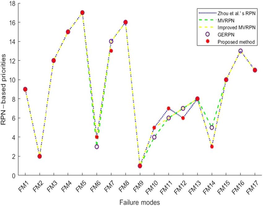
Experimental result of application 2. The comparison of the ranking result with other methods( MVRPN54,
Improved MVRPN48, GERPN55, Zhou et al.’s m ethod56) is shown in Fig. 4. The ranking result is very close to
Scientific Reports | (2022) 12:6812 | https://doi.org/10.1038/s41598-022-10828-2 8
Vol:.(1234567890)www.nature.com/scientificreports/
Figure 3. RPN values of Li and Chen’s method and the proposed method.
Risk Expert1 Expert2 Expert3
m(3)=0.4 m(3)=0.9 m(3)=0.8
O
m(4)=0.6 m(4)=0.1 m(4)=0.2
m(6)=0.1 m(6)=0.1 m(6)=0.1
S m(7)=0.8 m(7)=0.8 m(7)=0.8
m(8)=0.1 m(8)=0.1 m(8)=0.1
m(1)=0.1 m(1)=0.1 m(1)=0.1
D m(2)=0.8 m(2)=0.8 m(2)=0.8
m(3)=0.1 m(3)=0.1 m(3)=0.1
Table 9. belief structure of the first failure mode in application two.
Item FM1 FM2 FM3 FM4 FM5 FM6 FM7 FM8 FM9
RPN values 1.6858 2.3881 1.1111 0.6293 0.1554 2.2222 0.7778 0.5896 2.8293
ranking 9 2 12 15 17 4 13 16 1
Item FM10 FM11 FM12 FM13 FM14 FM15 FM16 FM17
RPN values 2.2222 1.8519 2.0279 1.8370 2.2370 1.5280 0.6983 1.2224
ranking 5 7 6 8 3 10 14 11
Table 10. The RPN values and ranking result.
the other methods, especially exactly the same as Zhou et al.’s method, which makes the usability of the method
further verified. As for the comparison of the RPN values, it is shown in Table 11. The RPN values of this method
are generally smaller than other RPN values. In case where all the assessments are different, other methods pro-
duces 5 same RPN values ( FM6 and FM10, FM11, FM12 and FM13), and this method produces only 2 same RPN
values(FM6 and FM10). The reason for this gap is the way experts are assigned weight.
Discussion. In general, the feasibility of the new method is verified by the above cases. One characteristic
of this method is that the RPN value generated is small, but it does not affect the final sorting result. Compared
with other methods, the new method is less likely to produce the same RPN values, which can better overcome
the defects of the traditional FMEA and make the evaluation more accurate. In addition, this method also has
some issues that need to be improved. The uncertainty between assessments of the same risk factor can represent
the weights of the experts, but the uncertainty between assessments of different risk factors cannot represent the
weights of different risk factors. Other uncertainty measures can be introduced into this method to measure the
weight between different risk factors.
Conclusion
The uncertainty of expert assessment has always been an inevitable problem in risk management. Due to the
effectiveness of FMEA in risk assessment, managers pay more and more attention to the accuracy of FMEA in
failure mode assessment to ensure the safe operation of the target system. Therefore, the traditional FMEA has
Scientific Reports | (2022) 12:6812 | https://doi.org/10.1038/s41598-022-10828-2 9
Vol.:(0123456789)www.nature.com/scientificreports/
Figure 4. Ranking of failure modes with different methods.
Item Zhou et al.’s RPN MVRPN Improved MVRPN GERPN Proposed method
FM1 46.4875 42.56 42.56 3.4910 1.6858
FM2 64.7921 64.00 64.05 3.9994 2.3881
FM3 30.0000 30.00 30.00 3.1069 1.1111
FM4 17.5822 18.00 17.97 2.6205 0.6293
FM5 3.6671 4.17 3.14 1.6095 0.1554
FM6 60.0000 60.00 60.00 3.9143 2.2222
FM7 21.0000 21.00 21.00 2.7586 0.7778
FM8 16.2000 15.00 15.00 2.4660 0.5896
FM9 70.5947 78.92 79.57 4.2881 2.8293
FM10 60.0000 60.00 60.00 3.9143 2.2222
FM11 50.0000 50.00 50.00 3.6836 1.8519
FM12 53.8039 50.00 50.00 3.6836 2.0279
FM13 49.3333 50.00 50.00 3.6836 1.8370
FM14 60.6337 60.00 60.04 3.9143 2.2370
FM15 41.9161 42.00 42.09 3.4756 1.5280
FM16 21.2967 23.88 23.86 2.8794 0.6983
FM17 31.2810 30.05 30.05 3.1089 1.2224
Table 11. A comparison of RPN values.
great limitations. At the same time, effective methods are also needed to improve the problems of the traditional
FMEA.
This work proposed a method based on the divergence measure to deal with the uncertainty of expert assess-
ment. This method transforms the uncertainty of experts’ subjective assessment into experts’ weight, and attempts
to improve the accuracy of assessment from the perspective of experts’ weight. At the same time, the divergence
measure highlights the correlation between assessments, so that the assessments are no longer isolated. Finally,
a case of a steel plate production process is used to verify the practicability of this method, and excellent results
are obtained.
The core idea in this work is that by using the divergence measure to obtain the divergence between assess-
ments and converting this divergence into the support degree of assessments, the support degree will repre-
sent the weight of experts. In the following research, we can apply this method to other fields to deal with the
uncertainty of subjective assessments and consider introducing information entropy to measure the quantity of
information in assessments to improve this method from the perspective of the weighted risk factor. In addition,
the fusion of different pieces of evidence with potential conflict has always been an open issue in the Dempster-
Shafer evidence theory. Thus, we can improve this method and apply it to the fusion of conflicting assessments.
Data availability
All data generated or analysed during this study are included in this published article.
Scientific Reports | (2022) 12:6812 | https://doi.org/10.1038/s41598-022-10828-2 10
Vol:.(1234567890)www.nature.com/scientificreports/
Received: 7 February 2022; Accepted: 13 April 2022
References
1. Wang, Z., Ran, Y., Chen, Y., Yu, H. & Zhang, G. Failure mode and effects analysis using extended matter-element model and ahp.
Comput. Ind. Eng. 140, 106233 (2020).
2. Wu, Z., Liu, W., & Nie, W. Literature review and prospect of the development and application of fmea in manufacturing industry,
Int. J. Adv. Manuf. Technol. 1–28 (2021).
3. Jones, M., Fretz, K., Kubota, S., Smith, & C. A. The use of the expanded fmea in spacecraft fault management, in 2018 Annual
Reliability and Maintainability Symposium (RAMS), IEEE, pp. 1–6 (2018).
4. Gueorguiev, T., Kokalarov, M., & Sakakushev, B. Recent trends in fmea methodology, in 2020 7th International Conference on
Energy Efficiency and Agricultural Engineering (EE & AE), IEEE, pp. 1–4 (2020).
5. Warnick, R. E., Lusk, A. R., Thaman, J. J., Levick, E. H. & Seitz, A. D. Failure mode and effects analysis (fmea) to enhance the safety
and efficiency of gamma knife radiosurgery. J. Radiosurg. SBRT 7, 115 (2020).
6. Permana, R. A., Ridwan, A. Y., Yulianti, F., & Kusuma, P. G. A. Design of food security system monitoring and risk mitigation of
rice distribution in indonesia bureau of logistics, in 2019 IEEE 13th International Conference on Telecommunication Systems,
Services, and Applications (TSSA), IEEE, pp. 249–254.
7. Hendiani, S., Mahmoudi, A. & Liao, H. A multi-stage multi-criteria hierarchical decision-making approach for sustainable supplier
selection. Appl. Soft Comput. 94, 106456 (2020).
8. Brun, A., & Savino, M. M. Assessing risk through composite fmea with pairwise matrix and markov chains, Int. J. Qual. Reliab.
Manag. (2018).
9. Park, J., Park, C. & Ahn, S. Assessment of structural risks using the fuzzy weighted euclidean fmea and block diagram analysis.
Int. J. Adv. Manuf. Technol. 99(9), 2071–2080 (2018).
10. Wu, J., Tian, J. & Zhao, T. Failure mode prioritization by improved rpn calculation method, in 2014 Reliability and Maintainability
Symposium, pp. 1–6.
11. Zhang, H., Dong, Y., Palomares-Carrascosa, I. & Zhou, H. Failure mode and effect analysis in a linguistic context: a consensus-
based multiattribute group decision-making approach. IEEE Trans. Reliab. 68, 566–582 (2018).
12. Subriadi, A. P. & Najwa, N. F. The consistency analysis of failure mode and effect analysis (fmea) in information technology risk
assessment. Heliyon 6, e03161 (2020).
13. Yazdi, M. Improving failure mode and effect analysis (fmea) with consideration of uncertainty handling as an interactive approach.
Int. J. Interact. Des. Manuf. (IJIDeM) 13, 441–458 (2019).
14. Nguyen, H. A new aggregation operator for intuitionistic fuzzy sets with applications in the risk estimation and decision making
problem, in 2020 IEEE International Conference on Fuzzy Systems (FUZZ-IEEE), IEEE, pp. 1–8.
15. Kabir, S. & Papadopoulos, Y. A review of applications of fuzzy sets to safety and reliability engineering. Int. J. Approx. Reason. 100,
29–55 (2018).
16. Wei, K., Geng, J. & Xu, S. Fmea method based on fuzzy theory and ds evidence theory. J. Syst. Eng. Electron. 41, 2662–2668 (2019).
17. Shi, H., Wang, L., Li, X.-Y. & Liu, H.-C. A novel method for failure mode and effects analysis using fuzzy evidential reasoning and
fuzzy petri nets, Journal of Ambient Intelligence and Humanized. Computing 11, 2381–2395 (2020).
18. Fan, C., Zhu, Y., Li, W. & Zhang, H. Consensus building in linguistic failure mode and effect analysis: a perspective based on
prospect theory. Qual. Reliab. Eng. Int. 36, 2521–2546 (2020).
19. Liu, B. & Deng, Y. Risk evaluation in failure mode and effects analysis based on d numbers theory. Int. J. Comput. Commun. Control
14, 672–691 (2019).
20. Ghoushchi, S. J., Gharibi, K., Osgooei, E., Ab Rahman, M. N. & Khazaeili, M. Risk prioritization in failure mode and effects analysis
with extended swara and moora methods based on z-numbers theory. Informatica 32, 41–67 (2021).
21. Seiti, H., Fathi, M., Hafezalkotob, A., Herrera-Viedma, E. & Hameed, I. A. Developing the modified r-numbers for risk-based
fuzzy information fusion and its application to failure modes, effects, and system resilience analysis (fmesra). ISA Trans. 113, 9–27
(2021).
22. Tang, M. & Liao, H. Failure mode and effect analysis considering the fairness-oriented consensus of a large group with core-
periphery structure. Reliab. Eng. Syst. Saf. 215, 107821 (2021).
23. Nie, W., Liu, W., Wu, Z., Chen, B. & Wu, L. Failure mode and effects analysis by integrating bayesian fuzzy assessment number
and extended gray relational analysis-technique for order preference by similarity to ideal solution method. Qual. Reliab. Eng. Int.
35, 1676–1697 (2019).
24. Gul, M., Yucesan, M. & Celik, E. A manufacturing failure mode and effect analysis based on fuzzy and probabilistic risk analysis.
Appl. Soft Comput. 96, 106689 (2020).
25. Liu, Z., Sun, L., Guo, Y., & Kang, J. Fuzzy fmea of floating wind turbine based on related weights and topsis theory, in 2015 Fifth
International Conference on Instrumentation and Measurement, Computer, Communication and Control (IMCCC), IEEE, pp.
1120–1125 (2015).
26. Wang, L., Hu, Y.-P., Liu, H.-C. & Shi, H. A linguistic risk prioritization approach for failure mode and effects analysis: a case study
of medical product development. Qual. Reliab. Eng. Int. 35, 1735–1752 (2019).
27. Wu, D. & Tang, Y. An improved failure mode and effects analysis method based on uncertainty measure in the evidence theory.
Qual. Reliab. Eng. Int. 36, 1786–1807 (2020).
28. Tang, Y., Zhou, D. & Chan, F. T. Amwrpn: Ambiguity measure weighted risk priority number model for failure mode and effects
analysis. IEEE Access 6, 27103–27110 (2018).
29. Ouyang, L., Zheng, W., Zhu, Y. & Zhou, X. An interval probability-based fmea model for risk assessment: a real-world case. Qual.
Reliab. Eng. Int. 36, 125–143 (2020).
30. Zheng, H. & Tang, Y. Deng entropy weighted risk priority number model for failure mode and effects analysis. Entropy 22, 280
(2020).
31. Zhou, H., Yang, Y.-J., Huang, H.-Z., Li, Y.-F. & Mi, J. Risk analysis of propulsion system based on similarity measure and weighted
fuzzy risk priority number in fmea. Int. J. Turbo Jet-Engines 38, 163–172 (2021).
32. Pang, J., Dai, J., & Qi, F. A potential failure mode and effect analysis method of electromagnet based on intuitionistic fuzzy number
in manufacturing systems, Math. Prob. Eng. 2021 (2021).
33. Jin, C., Ran, Y. & Zhang, G. An improving failure mode and effect analysis method for pallet exchange rack risk analysis. Soft.
Comput. 25, 15221–15241 (2021).
34. Song, Y. & Wang, X. A new similarity measure between intuitionistic fuzzy sets and the positive definiteness of the similarity
matrix. Pattern Anal. Appl. 20, 215–226 (2017).
35. Liu, Z.-G., Huang, L.-Q., Zhou, K. & Denoeux, T. Combination of transferable classification with multisource domain adaptation
based on evidential reasoning. IEEE Trans. Neural Netw. Learn. Syst. 32, 2015–2029 (2021).
36. Liu, Z., Zhang, X., Niu, J. & Dezert, J. Combination of classifiers with different frames of discernment based on belief functions.
IEEE Trans. Fuzzy Syst. 29, 1764–1774 (2021).
37. Deng, Y. Uncertainty measure in evidence theory, Science China. Inf. Sci. 63, 1–19 (2020).
Scientific Reports | (2022) 12:6812 | https://doi.org/10.1038/s41598-022-10828-2 11
Vol.:(0123456789)www.nature.com/scientificreports/
38. Wang, X. & Song, Y. Uncertainty measure in evidence theory with its applications. Appl. Intell. 48, 1672–1688 (2018).
39. Jousselme, A.-L., Liu, C., Grenier, D. & Bossé, É. Measuring ambiguity in the evidence theory. IEEE Trans. Syst. Man Cybern. Part
A Syst. Hum. 36, 890–903 (2006).
40. Deng, Z. & Wang, J. Measuring total uncertainty in evidence theory. Int. J. Intell. Syst. 36, 1721–1745 (2021).
41. Xu, S. et al. A novel divergence measure in dempster-shafer evidence theory based on pignistic probability transform and its
application in multi-sensor data fusion. Int. J. Distrib. Sens. Netw. 17, 15501477211031472 (2021).
42. Jiang, W. A correlation coefficient for belief functions. Int. J. Approx. Reason. 103, 94–106 (2018).
43. Zhou, Q. & Deng, Y. Fractal-based belief entropy. Inf. Sci. 587, 265–282 (2022).
44. Xiao, F. Multi-sensor data fusion based on the belief divergence measure of evidences and the belief entropy. Inf. Fusion 46, 23–32
(2019).
45. Lin, J. Divergence measures based on the shannon entropy. IEEE Trans. Inf. Theory 37, 145–151 (1991).
46. Dempster, A. P. Upper and lower probabilities induced by a multi-valued mapping. Ann. Math. Stat. 38, 325–339 (1967).
47. Shafer, G. A Mathematical Theory of Evidence (Princeton University Press, Princeton, 1976).
48. Su, X., Deng, Y., Mahadevan, S. & Bao, Q. An improved method for risk evaluation in failure modes and effects analysis of aircraft
engine rotor blades. Eng. Fail. Anal. 26, 164–174 (2012).
49. Bian, T., Zheng, H., Yin, L. & Deng, Y. Failure mode and effects analysis based on d numbers and topsis. Qual. Reliab. Eng. Int. 34,
501–515 (2018).
50. Xiao, F. A new divergence measure for belief functions in d-s evidence theory for multisensor data fusion. Inf. Sci. 514, 462–483
(2020).
51. Wang, H., Deng, X., Jiang, W. & Geng, J. A new belief divergence measure for dempster-shafer theory based on belief and plausibil-
ity function and its application in multi-source data fusion. Eng. Appl. Artif. Intell. 97, 104030 (2021).
52. Li, Z. & Chen, L. A novel evidential fmea method by integrating fuzzy belief structure and grey relational projection method. Eng.
Appl. Artif. Intell. 77, 136–147 (2019).
53. Vahdani, B., Salimi, M. & Charkhchian, M. A new fmea method by integrating fuzzy belief structure and topsis to improve risk
evaluation process. Int. J. Adv. Manuf. Technol. 77, 357–368 (2015).
54. Yang, J., Huang, H.-Z., He, L.-P., Zhu, S.-P. & Wen, D. Risk evaluation in failure mode and effects analysis of aircraft turbine rotor
blades using dempster-shafer evidence theory under uncertainty. Eng. Fail. Anal. 18, 2084–2092 (2011).
55. Zhou, D., Tang, Y. & Jiang, W. A modified model of failure mode and effects analysis based on generalized evidence theory. Math.
Probl. Eng. 2016, 1–11 (2016).
56. Zhou, X. & Tang, Y. Modeling and fusing the uncertainty of fmea experts using an entropy-like measure with an application in
fault evaluation of aircraft turbine rotor blades. Entropy 20, 864 (2018).
Author contributions
Y.L. and Y.T. designed the research and wrote the manuscript text. All authors reviewed the manuscript.
Funding
The work is supported by the National Key Research and Development Project of China (Grant No.
2020YFB1711900). There was no additional external funding received for this study.
Competing interests
The authors declare no competing interests.
Additional information
Correspondence and requests for materials should be addressed to Y.T.
Reprints and permissions information is available at www.nature.com/reprints.
Publisher’s note Springer Nature remains neutral with regard to jurisdictional claims in published maps and
institutional affiliations.
Open Access This article is licensed under a Creative Commons Attribution 4.0 International
License, which permits use, sharing, adaptation, distribution and reproduction in any medium or
format, as long as you give appropriate credit to the original author(s) and the source, provide a link to the
Creative Commons licence, and indicate if changes were made. The images or other third party material in this
article are included in the article’s Creative Commons licence, unless indicated otherwise in a credit line to the
material. If material is not included in the article’s Creative Commons licence and your intended use is not
permitted by statutory regulation or exceeds the permitted use, you will need to obtain permission directly from
the copyright holder. To view a copy of this licence, visit http://creativecommons.org/licenses/by/4.0/.
© The Author(s) 2022
Scientific Reports | (2022) 12:6812 | https://doi.org/10.1038/s41598-022-10828-2 12
Vol:.(1234567890)You can also read