Method of Local Corrections Solver for Manycore Architectures - EECS Berkeley
←
→
Page content transcription
If your browser does not render page correctly, please read the page content below
Method of Local Corrections Solver for Manycore
                 Architectures

             Brian Van Straalen

             Electrical Engineering and Computer Sciences
             University of California at Berkeley

             Technical Report No. UCB/EECS-2018-122
             http://www2.eecs.berkeley.edu/Pubs/TechRpts/2018/EECS-2018-122.html

             August 10, 2018
Copyright © 2018, by the author(s).
                             All rights reserved.

Permission to make digital or hard copies of all or part of this work for
personal or classroom use is granted without fee provided that copies are
not made or distributed for profit or commercial advantage and that copies
bear this notice and the full citation on the first page. To copy otherwise, to
republish, to post on servers or to redistribute to lists, requires prior specific
permission.

                               Acknowledgement

For my Father. August 1930-August 2018. You held on for Doctorate Dad.
Thanks.

I would not have gotten to hear with my advisor's heroics. Thanks Phil.
Method of Local Corrections Solver for Manycore Architectures
by
Brian Van Straalen
A dissertation submitted in partial satisfaction of the
requirements for the degree of
Doctor of Philosophy
in
Computer Science
and the Designated Emphasis
in
Computational and Data Science and Engineering
in the
Graduate Division
of the
University of California, Berkeley
Committee in charge:
Professor Phillip Colella, Chair
Professor James Demmel
Professor John Strain
Summer 2018Method of Local Corrections Solver for Manycore Architectures
Copyright 2018
by
Brian Van Straalen1
Abstract
Method of Local Corrections Solver for Manycore Architectures
by
Brian Van Straalen
Doctor of Philosophy in Computer Science
University of California, Berkeley
Professor Phillip Colella, Chair
Microprocessor designs are now changing to reflect the ending of Dennard Scaling. This
leads to a reconsideration of design tradeoffs for designing discretization methods for PDEs
based on simplified performance models like Roofline.
In this work we carry out an end-to-end analysis and implementation study on a Cray
XC40 with Intel R XeonTM E5-2698 v3 processors for the Method of Local Corrections
(MLC). MLC is a non-iterative method for solving Poisson’s Equation on locally rectan-
gular meshes. The Roofline model predicts that MLC should have faster time to solution
than traditional iterative methods such as Geometric Multigrid. We find that Roofline is a
useful guide for performance engineering and obtain performance within a factor of 3 the
Roofline performance upper bound. We determine that the algorithm is limited by identified
architectural features that are not captured in the Roofline model, are quantifiable, and can
be addressed in future implementations.i Contents Contents i List of Figures iii List of Tables v 1 Introduction 2 1.1 Hardware Trends . . . . . . . . . . . . . . . . . . . . . . . . . . . . . . . . . 2 1.2 Poisson’s Equation . . . . . . . . . . . . . . . . . . . . . . . . . . . . . . . . 4 1.3 Fast Solvers for Poisson’s Equation . . . . . . . . . . . . . . . . . . . . . . . 5 1.4 Thesis . . . . . . . . . . . . . . . . . . . . . . . . . . . . . . . . . . . . . . . 6 2 Algorithm 9 2.1 Discretization . . . . . . . . . . . . . . . . . . . . . . . . . . . . . . . . . . . 9 2.2 The Two-Level Method of Local Corrections . . . . . . . . . . . . . . . . . . 11 2.3 Analogy with FAS . . . . . . . . . . . . . . . . . . . . . . . . . . . . . . . . 14 2.4 General Multilevel Algorithm . . . . . . . . . . . . . . . . . . . . . . . . . . 15 2.5 Hockney’s Algorithm: The Heart of MLC . . . . . . . . . . . . . . . . . . . . 19 3 Software and Tools 26 3.1 Block-Structured Adaptive Mesh Refinement . . . . . . . . . . . . . . . . . . 26 3.2 Modalities of Parallel Processing . . . . . . . . . . . . . . . . . . . . . . . . . 27 3.3 Chombo . . . . . . . . . . . . . . . . . . . . . . . . . . . . . . . . . . . . . . 28 3.4 FFTW . . . . . . . . . . . . . . . . . . . . . . . . . . . . . . . . . . . . . . . 29 3.5 HDF5 . . . . . . . . . . . . . . . . . . . . . . . . . . . . . . . . . . . . . . . 29 4 Performance Models 30 4.1 Opportunities for Optimization . . . . . . . . . . . . . . . . . . . . . . . . . 31 5 Experiments 34 5.1 Correctness of implementation . . . . . . . . . . . . . . . . . . . . . . . . . . 34 6 Conclusions 52
ii

A Notation                                                     55

B Lh19 and Lh27 Mehrstellen Discretizations of the Laplacian   57

C Deriving Hockney’s Algorithm                                 58

D Computing PL (f h )                                          60

Bibliography                                                   62
iii
List of Figures
1.1 Single Socket Roofline plots for NERSC Hopper (Cray XE6) and Edison (Cray
XC30) platforms. Generating using the Empirical Roofline Toolkit [50]. The
theoretical peak performance from hardware specifications is given in green. . . 4
1.2 Single Socket Roofline plots for NERSC Cori (Cray XC40 Haswell nodes). Gener-
ated using the Empirical Roofline Toolkit [50]. The theoretical peak performance
from hardware specifications is given in green. . . . . . . . . . . . . . . . . . . . 8
2.1 Regions about the patch k. . . . . . . . . . . . . . . . . . . . . . . . . . . . . . 12
2.2 2D Convolution . . . . . . . . . . . . . . . . . . . . . . . . . . . . . . . . . . . . 21
5.1 Adaptive mesh hierarchy for oscillatory problem. 3 level of refinement. Factor
of 4 refinement ratio. Each outlined patch is a 33x33x33 set of structured grid
points. The base grid dimensions are varied through the course of a convergence
study while the grid geometries and ratios are preserved. . . . . . . . . . . . . . 36
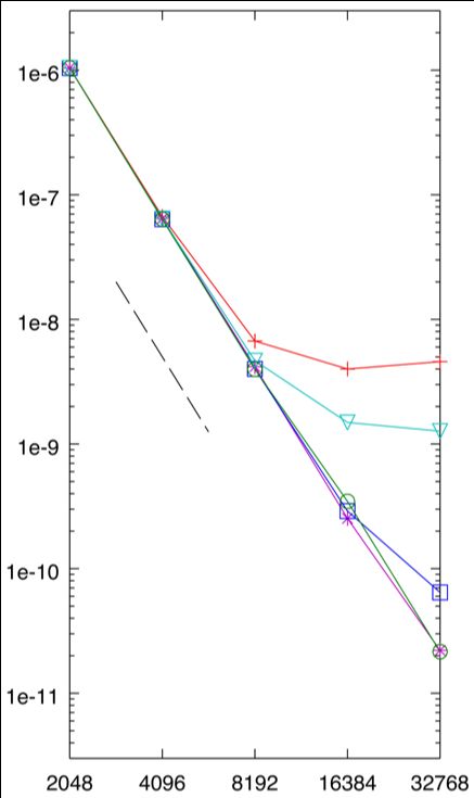
5.2 + 27-pt operator N = 323 , α = 2.25, β = 3.25, 5 27-pt operator N = 643 , α =
1.625, β = 2.125, 27-pt operator N = 643 , α = 2.25, β = 3.25, ∗ 117-pt operator
N = 323 , α = 2.25, β = 3.25, 117-pt operator N = 643 , α = 2.25, β = 3.25.
1
X-axis is h of the base grid. Max norm error. 4th-order slope drawn as dashed
line. . . . . . . . . . . . . . . . . . . . . . . . . . . . . . . . . . . . . . . . . . . 37
5.3 Scaling results for Cori Haswell XC40 supercomputer. N=333 , 27-point operator,
3rd-order Legendre Polynomial expansions, α=2.25, β=3.25. Vertical axis is time,
in seconds. Horizontal axis is total number of cores. . . . . . . . . . . . . . . . . 38
5.4 Experimentally-derived bandwidth measurements of 1 node (2 sockets, 32 cores)
experimental platform for 2 FLOP computational kernel using 4 MPI ranks, each
with 8 OpenMP threads . . . . . . . . . . . . . . . . . . . . . . . . . . . . . . . 42
5.5 Experimentally-derived bandwidth measurements of 1 node (2 sockets, 32 cores)
experimental platform for 2 FLOP computational kernel using 16 MPI ranks,
each with 2 OpenMP threads . . . . . . . . . . . . . . . . . . . . . . . . . . . . 43iv
F
5.6 Hockney Convolution Worksheet DRAM Arithmetic Intensity AI= B =61: 27-
point Laplacian operator, zero structure exploited, steps 3-5 (k-pencils) opera-
tions fused, ns =33, nd =97. 1. Assumes that a single MPI rank will perform
many Hockney convolutions and the load of Ĝ is ammortized away. 2. These
operations share a common work array with inverse J-transform and so do not
count towards the total working set. 3. This would be the peak working set size
if we did not block and fuse the k-direction operations. . . . . . . . . . . . . . . 44
5.7 Experimentally-derived bandwidth measurements of 1 node (2 sockets, 32 cores)
experimental platform for 32 FLOP computational kernel using 4 MPI ranks,
each with 8 OpenMP threads . . . . . . . . . . . . . . . . . . . . . . . . . . . . 48v
List of Tables
2.1 Steps for coarse-grained Hockney transforms. The column headings are a naming
convention used by the FFTW API and described in section 3.4. . . . . . . . . . 23
2.2 Steps for fine-grained threaded Hockney transforms. A new column now appears
that describes how threads are distributed across the operations within the trans-
form. . . . . . . . . . . . . . . . . . . . . . . . . . . . . . . . . . . . . . . . . . . 24
2.3 Steps for compact fine-grained threaded Hockney transforms . . . . . . . . . . . 24
4.1 big O Complexity for a given p for GMG V-cycle, FMG, FFT and MLC. N grid
points, p processors. d refers to the amount of domain decomposition used in
MLC. FFT is done as a single large FFT operation, while MLC first decomposes
the domain into d compact disjoint regions. . . . . . . . . . . . . . . . . . . . . 31
4.2 Computational Complexity per finest level grid point for Method of Local Cor-
rections. Refinement ratio r, N grid points in BR , Γ: number of basis functions
for polynomial expansion. qn are the number of points in the Laplacian stencil.
* f h loaded in step 1 gets reused in step 2 and we assume that Ĝ can fit inside
the near-memory working set and does not need to be reloaded across subsequent
convolution operations. . . . . . . . . . . . . . . . . . . . . . . . . . . . . . . . . 31
4.3 Computational Complexity per grid point for 2-level Geometric Multigrid (GMG).
Assume proper MG convergence rates and a standard 4 relaxations V-cycle for
10 iterations to have comparable error tolerance as MLC. qn points in Laplacian
stencil. Assumes a communication-avoiding implementation with extra ghost
cells. The relaxation steps have been fused into a skewed loop (wavefront or di-
amond). Assumes no agglomeration, so not a true V-cycle, just the finest level
solver . . . . . . . . . . . . . . . . . . . . . . . . . . . . . . . . . . . . . . . . . 32
4.4 Multigrid vs MLC. α = 2.25, β = 3.25, N = 333 , r = 4, qn = 27, Γ = 20. The
dominant compute kernel Hockney Transform is shown in red. You have fractional
values for MLC as Φ is subsampled on output to adjacent MLCFaces and the
coarser grid . . . . . . . . . . . . . . . . . . . . . . . . . . . . . . . . . . . . . . 33
4.5 A restatement of Table 4.4 expressed in common units of cycles for the Edison
XC30 platform within a single node. FLOPS are turned into cycles using the
peak FMA performance. load/stores are turned into a common unit of cycles
based on peak DRAM bandwith. . . . . . . . . . . . . . . . . . . . . . . . . . . 33vi
5.1 Extracted performance call-graph for Variant 1. Flat MPI execution . . . . . . . 39
5.2 Performance breakdown for Variant 3 of MLC . . . . . . . . . . . . . . . . . . . 41
5.3 Performance breakdown for Variant 4 of MLC . . . . . . . . . . . . . . . . . . . 45
5.4 HPGMG Performance on uniform grid with domain decomposition and hybrid
MPI+OpenMP execution . . . . . . . . . . . . . . . . . . . . . . . . . . . . . . 46
5.5 SDE Output from Variant 4 Kernel Benchmark . . . . . . . . . . . . . . . . . . 50
A.1 Notation . . . . . . . . . . . . . . . . . . . . . . . . . . . . . . . . . . . . . . . . 562
Chapter 1
Introduction
1.1 Hardware Trends
Microprocessor design in the past decade have been shaped by two dominant physical effects:
Our continued ability to reduce feature size as discussed in the ITRS: The international
technology roadmap for semiconductors [43] and the end of Dennard Scaling [30, 32]. Dennard
(1974) observed that voltage and current should be proportional to the linear dimensions
of a transistor. Thus, as transistors shrank, so did necessary voltage and current; power is
proportional to the area of the transistor. So smaller features were matched by lower power
trends and the product of the two, power density, remained stable. Dennard scaling ignored
the leakage current and threshold voltage, which establish a baseline of power per transistor.
Now, as transistors get smaller, power density increases. Thus we have the power wall that
has limited practical processor frequency to around 4 GHz since 2006. This kicked off our
current era of using more processing cores that distributed the thermal load, and fewer
transistors dedicated to mitigating memory latency, which have higher power density. These
changes were well documented in the National Academy Study The Future of Computing
Performance[37]. The general term for this architectural shift is manycore.
To capture this complicated architectural landscape it is helpful to reference more simpli-
fied computing abstractions and performance models. The Roofline model [67, 66] describes
the upper limits of attainable performance in terms of bandwidth and arithmetic operations.
The name Roofline is evocative of a ceiling on attainable performance for algorithms that
can be expressed as a streaming computation. For a given ratio of arithmetic operations
that need to be performed and bytes of memory that need to be accessed, and a data work-
ing set size, the Roofline predicts the maximum performance that can be obtained from an
optimal algorithm implementation. The trend can be seen in two successive generations of
Intel R microprocessor-based supercomputer platforms from the Department of Energy Na-
tional Energy Research Supercomputer Center in figure 1.1. The vertical axis is in units of
GFLOP/s. The horizontal axis is the arithmetic intensity, specified as the number of FLOPs
performed per byte of memory accessed. The slanted bandwidth lines (L1, L2, L3, DRAM)CHAPTER 1. INTRODUCTION 3
all have a slope of 1/8 (8 being the number of bytes in a double-precision floating-point
data value). Each line represents the peak GFLOP/s acheivable for a streaming compute
kernel that is bandwidth-bound whose working set fits with the named level of the cache
hieararchy. Bandwidth-bound means that the processor is capable of executing floating-point
operations faster, but the memory subsystem is not capable of delivering bytes to and from
the functional units to keep them fully active. The processor will execute some number
of NOP instructions while waiting for outstanding load/store instructions to complete. The
horizontal lines represent the maximum GFLOP/s achievable set by the ability of the pro-
cessor to execute floating-point instructions. Multiply/Add shows the peak performance for
motifs that utilitze a Fused-Multiply-Add instruction. Add stands in for all other instruc-
tions that are the eqivalent of a single floating-point operation. Computional motifs that are
constrained by the horizontal red lines are said to be Compute-bound. The Roofline defines a
peak performance attainable. Many architectural complexities are elided here, but all other
features will only lower performance relative to this performance envelope.
Several classic HPC motifs are plotted in these Roofline plots in magenta: Algebraic
Multigrid/Sparse Matrix-Vector Multiply (AMG/SpMV), Geometric Multigrid (GMG), Ge-
ometric Multigrid with the more computationally dense GMG scheme where several core
computational phases have been manually fused and tuned (GMG (fused)), Fast Fourier
Transform, both small (FFT(1K)), and large (FFT (8K)) computed as 5N log2 (N )/4 · 8 · N ,
and Dense Double-Precision Matrix-Matrix Multiply (DGEMM, m·n = 128). In the Roofline
Model a computational motif is entirely characterized by its arithmetic intensity, to these
are shown as vertical lines. For example, we can make a prediction for a Sparse Matrix-
Vector multiply kernel on the Edison platform where the working set fits entirely in the L2
level of cache. We follow the AMG/SpMV line that defines the arithmetic intensity of this
algorithm (AI=0.125) upwards until we encounter the rate-limiting ceiling on performance,
which shows that these algorithm motifs are bandwidth-bound by the available L2 band-
width and the expected upper bound performance can be read from the intersection of with
the L2 bandwidth limit (in this case roughly 63 GFLOPS).
The Roofline model highlights the need to place less emphasis on algorithms that empha-
size minimum floating-point and towards algorithms that minimize data movement. This
concept has been well studied for dense and sparse communication-avoiding linear algebra
[29, 4, 28] and extended to what Demmel and Ballard refers to computations that “smell
like” triply-nested loops [11, 10]. For algorithms that have a SpMV-kernel at their core you
can see from the Roofline model that communication-avoiding should be the entire focus.
We will investigate the utility of a Roofline performance model in guiding the development
of a new fast Poisson solver algorithm.CHAPTER 1. INTRODUCTION 4
Single Socket Roofline for NERSC’s Hopper (Cray XE6) Single Socket Roofline for NERSC’s Edison (Cray XC30)
1000 1000
GMG/Cheby (fused)
GMG/Cheby
AMG/SpMV
GFLOP/s Spec
FFT (1K)
FFT (8K)
DGEMM
Multiply/Add
L1 pec
100 100 Add
S
L1
L2
GFLOP/s Spec
GFLOP/s
GFLOP/s
L3
ec
Multiply/Add
ec
Sp
Sp
AM
Add
AM
L1
R
D
L1
R
D
L2
10 10
GMG/Cheby (fused)
L3
ec
Sp
AM
AM
GMG/Cheby
AMG/SpMV
R
R
D
D
FFT (1K)
FFT (8K)
DGEMM
1 1
0.01 0.1 1 10 100 0.01 0.1 1 10 100
FLOP/Byte FLOP/Byte
Figure 1.1: Single Socket Roofline plots for NERSC Hopper (Cray XE6) and Edison (Cray
XC30) platforms. Generating using the Empirical Roofline Toolkit [50]. The theoretical peak
performance from hardware specifications is given in green.
1.2 Poisson’s Equation
We are seeking to solve Poisson’s Equation in free space
∆(Φ) = f where supp(f ) = D bounded domain in R3 (1.1)
Φ, f : R3 → R
Q 1
Φ(x) = +o as ||x|| → ∞ (1.2)
4π||x|| ||x||
Z
Q= f dx
D
which can be expressed as convolution with the Green’s function
Z
1
Φ(x) = G(x − y)f (y)dy ≡ (G ∗ f )(x) , G(x) = . (1.3)
D 4π||x||
We seek solutions to these forms of equations on the emerging manycore computing
architectures.
A wide range of relevant scientific computing applications require the solution to Poisson’s
equation including gravity in cosmological and astrophysical models, electrostatic potential
in kinetic plasma physics and Coulomb potentials in molecular dynamics and projection
methods for solving viscous incompressible flows [21, 22, 51, 42].CHAPTER 1. INTRODUCTION 5
1.3 Fast Solvers for Poisson’s Equation
A simple and correct method for solving (1.3) would be to discretize space and compute the
integral with numerical quadrature. While correct this results in an O(N 2 ) algorithm where
N is the number of grid points. Expressing the discretization of equation (1.3) by finite-
difference methods and constructing a linear system of equations to solve also works and
Krylov-based iterative methods like preconditioned conjugate gradient can solve these well-
conditioned systems of equations in O(N k ) for k only lightly larger than 1. Unfortunately
even a small increment in k above 1 leads to a large increment in cost when N becomes
large.
Solutions to (1.3) have the property that Φ is a smooth function away from the support
of the charge D. Differentiating (1.3) we see that
w 1
∇ Φ(x) = O ||w||1 +1 (1.4)
l
where w = [w1 , w2 , w3 ], wi are non-negative integers, ||w||1 = w1 + w2 + w3 , and l = distance
between x and the support of f . The field induced by distant charges has derivatives that
decay like an inverse power law. Thus it should be possible to represent the the nonlocal
dependence of the field on the charge using less computational effort. This observation
underlies all fast Poisson solvers, and several algorithms have been developed that exploit
this property.
For a uniform rectangular grid discretization of Φ and f , the Fast Fourier Transform
(FFT) can be used to solve Poisson’s equation on a periodic domain, combined with one of
a number of techniques for correcting for the infinite-domain boundary conditions. The core
FFT solver takes 5N log2 (N ) floating-point operations. Distributed Fast Fourier Transform
Techniques [2, 5, 15] are efficient and fast.
Geometric Multigrid [63, 18] is an iterative method for solving grid-based discretizations
of Poisson’s equation. It uses local O(N ) relaxation techniques to reduce high-wave-number
components of the error, and the effect of the smooth non-local coupling is efficiently com-
puted by solving the equations on a coarsened grid, with iteration between the coarse and
fine representations to obtain the solution. The approach is applied recursively in refinement
level. This leads to an O(N ) method, where the constant depends on the specific discretiza-
tion of the Laplacian, but is at least 10x larger than the corresponding constant of 15 in
the FFT solver. However, geometric multigrid can be applied to a much broader range of
spatial discretizations, such as mapped grids and nested locally refined rectangular grids.
Multigrid has been shown to be scalable to O(100K) cores on homogeneous supercomputers
with O(109 ) unknowns[64].
The Fast Multipole Method (FMM)[39, 38, 33] and related tree-based fast Poisson solvers[12]
are numerical techniques that were developed to speed up the calculation of long-range forces
in the n-body problem. FMM does this by expanding the system Green’s function using a
multipole expansion. Recent implementations have shown good scaling on modern het-
erogeneous architectures [48]. The Generalized Fast Multipole Method [68] does exploit aCHAPTER 1. INTRODUCTION 6
uniform grid sampling and is not limited to problems that have an analytic Green’s function
but has several quadrature integrations at every step in the algorithm and has increasing
computational complexity and communication for higher degrees of accuracy.
In this work we will be investigating The Method of Local Corrections (MLC)
[46, 53] defined on structured hierarchically adaptive structured grids, commonly referred to
as Structured Adaptive Mesh Refinement (AMR) data layouts [3, 31, 60, 8, 24, 23]. MLC
breaks the integral form of equation (1.3) into near-field operations that are computed using
direct convolutions on small structured patches to neighbors, and a far-field contribution
that is solved on a coarser grid refinement. The coarser solve is handled with a similar
decomposition into near and far contributions on the next coarser grid.
MLC proceeds in three steps: (i) a loop over the fine disjoint patches and the computation
of local potentials induced by the charge restricted to those patches on sufficiently large
extensions of their support (downward pass); (ii) a global coarse-grid Poisson solve with a
right hand side computed by applying the coarse-grid Laplacian to the local potentials of
step (i) bottom solve; and (iii) a correction of the local solutions computed in step (i) on
the boundaries of the fine disjoint patches based on interpolating the global coarse solution
from which the contributions from the local solutions have been subtracted (upward pass).
These boundary conditions are propagated into the interior of the patches by performing
Dirichlet solves on each patch. This method is applied recursively to progressively coarser
grid refinements.
Structurally MLC is most closely related to Multigrid as it is deployed in AMR algorithms
[64]. There is a downward pass where a modified source term is generated, a bottom solve,
and an upward pass where corrections to the fine grid solution from the coarse-grid solutions
are interpolated. Parallel implementations are based on domain decomposition, and the
gridding structure is compatible with more general applications that use AMR grids and
require the solution to Poisson’s equation as a substep. MLC, unlike Multigrid, is not
iterative, and has as a compute kernel small batched FFTs to compute discrete convolutions,
rather than stencil operations.
Fast Multipole Methods are also similar to MLC in that they both directly utilize the
convolution form of Poisson’s Equation, and have a natural hierarchy of scales that leads to
a recursive traversal through the data structures. However, mapping the classic spherical
multipole basis onto AMR hierarchies adds many complexities of interpolation and quadra-
ture.
1.4 Thesis
At the core of MLC is the opportunity to trade-off more floating-point operations for less
data movement with the end result of faster time to solution with the coming hardware
trends. The near-field convolutions can be performed using the Fast-Fourier Transform us-
ing a variant of the Convolution Theorem and identities for turning linear convolutions into
circular convolutions. These convolution operations will be shown to dominate the compu-CHAPTER 1. INTRODUCTION 7
tation cost of the algorithm, and they can have highly efficient implementations on modern
manycore architectures. We want to assess to what extent we are capable of implementing
MLC up to its potential of a Roofline model. A look at figure 1.2 shows that for an algo-
rithm composed of collections of FFTs of roughly 2M elements should execute within the
floating-point dominated regime of a contemporary processor.
In this thesis we will study the performance potential of MLC theoretically in Chapter 4,
then implement and analyze several progressively improved implemenatations in Chapter 5
using a current HPC platform Cori at the NERSC supercomputer center. Cori has compute
nodes with Two 2.3 GHz 16-core Haswell processors per node. Each core has its own L1 and
L2 caches, with 64 KB (32 KB instruction cache, 32 KB data) and 256 KB, respectively;
there is also a 40-MB shared L3 cache per socket. Nodes are connected for distributed
computing using a Cray Aries high speed ”dragonfly” topology interconnect. The target
Roofline model for this work is given in figure 1.2.
Outline for Thesis
First we will define our numerical scheme for representing the discrete problem definition
from the continuous operator, a description of Hockney’s discrete convolution algorithm,
introduce domain decomposition, and then the Method of Local Corrections. Second a
performance model is given for the overall MLC algorithm and its key discrete convolution
kernel. Third we present descriptions of four algorithm variants, their measured performance,
and further performance analysis and motivations for each implementation variant. Finally,
a deep analysis of the current best algorithm implemented and future directions.CHAPTER 1. INTRODUCTION 8
Single Socket Roofline for NERSC’s Cori (Haswell partition Cray XC40)
1000 GFLOP/s Spec
Multiply/Add
Add
ec
L1 Sp
L1
L2
100
L3
e c
Sp
GFLOP/s
AM
R
D
AM
R
D
10
GMG/Cheby (fused)
GMG/Cheby
AMG/SpMV
FFT (2M)
FFT (1K)
DGEMM
1
0.01 0.1 1 10 100
FLOP/Byte
Figure 1.2: Single Socket Roofline plots for NERSC Cori (Cray XC40 Haswell nodes). Gen-
erated using the Empirical Roofline Toolkit [50]. The theoretical peak performance from
hardware specifications is given in green.9
Chapter 2
Algorithm
2.1 Discretization
Domain decomposition and Adaptive Structured Grids
We denote by Dh , Ω h · · · ⊂ Z3 grids with grid spacing h of discrete points in physical space:
{gh : g ∈ Dh }. Arrays of values defined over such sets will approximate functions on subsets
of R3 , i.e. if ψ = ψ(x) is a function on D ⊂ R3 , then ψ h [g] ≈ ψ(gh). We denote operators
on arrays over grids of mesh spacing h by Lh , ∆h , . . . ; Lh (φh ) : Dh → R. Such operators
0
are also defined on functions of x ∈ R3 , and on arrays defined on coarser grids φh , h =
0 0
N h0 , N ∈ N+ , by sampling: Lh (φ) ≡ Lh (S h (φ)), S h (φ)[g] ≡ φ(gh); Lh (φh ) ≡ Lh (S h (φh )),
0 0
S h (φh )[g] ≡ φh [N g].
For a rectangle D = [l, u], defined by its low and upper corners l, u ∈ Z3 , we define the
operators
G(D, r) = [l − (r, r, r), u + (r, r, r)], r ∈ Z
hj l k l u mi
C(D) = ,
Nref Nref
Throughout this paper, we will use Nref = 4 for the refinement ratio between levels.
The discrete Laplacian operator Lh
We begin our discussion presenting the finite difference discretizations of (1.3) that we will
be using throughout this work and some of their properties that pertain to the Method of
Local Corrections.
We are employing Mehrstellen discretizations [25] (also referred to as compact finite
difference discretizations) of the 3D Laplace operator
X
(∆h φh )g = as φhg+s , as ∈ R. (2.1)
s∈[−s,s]3CHAPTER 2. ALGORITHM 10
The associated truncation error τ h ≡ (∆h − ∆)(φ) = −∆h (φh − φ) for the Mehrstellen
discrete Laplace operator is of the form
q
2
−1
0 0
X
τ h (φ) = C2 h2 ∆(∆φ) + h2q L2q (∆φ) + hq Lq+2 (φ) + O(hq+2 ), (2.2)
q 0 =2
0
where q is even and L2q and Lq+2 are constant-coefficient differential operators that are
homogeneous, i.e. for which all terms are derivatives of order 2q 0 and q + 2, respectively. For
1
the 27-pt Laplacian operator considered here, C2 = 12 . In general, the truncation error is
2
O(h ). However, if ∆φ = 0 in a neighborhood of x,
τ h (φ)(x) = ∆h (φ)(x) = hq Lq+2 (φ)(x) + O(hq+2 ). (2.3)
In our specific numerical test cases we make use 27-point (Lh27 ) Mehrstellen stencil [61] that
is described in the Appendix (Section B), for which q = 6. In general, it is possible to
define operators for which s = b 4q c for any even q, using higher-order Taylor expansions and
repeated applications of the identity
∂ 2r φ ∂ 2r−2 X ∂ 2r
= (∆φ) − (φ).
∂x2rd ∂x2r−2
d 0
d 6=d
∂x 2r−2
d 0 ∂x 2
d
The discrete Green’s Function
With a definition of the discrete Laplacian operator we can specify the discrete Green’s
Function Gh from the definition:
Lh Gh = 0 when i 6= 0 (2.4)
=1 i=0 (2.5)
Given such a Gh then the following property is true:
X
(Gh ∗ f h ) = (∆h )−1 (f h ) ,(Gh ∗ f h )[g] ≡ h3 Gh [g − g 0 ]f [g 0 ]h (2.6)
g 0 ∈Z3
In traditional Green’s function solvers the analytic form of the Green’s Function in fre-
1
quency space Ĝ(k) = k2 −k 2 for the Laplacian operator is often used. The analytic Green’s
0
Function limits your overall algorithm accurac to just 2nd-order.
For simple operators, like the 2D 5- or 9-point Laplacian it is possible to use analytic
methods to compute the discrete Green’s function as done by Buneman [19]. While the
method can possibly be extended to higher-order schemes the procedure is cumbersome and
error prone. We need to compute an approximation to the discrete Green’s function Gh for
the 27-point operator, restricted to a domain of the form D = [−n, n]3 . We do this byCHAPTER 2. ALGORITHM 11
solving the following inhomogeneous Dirichlet problem on a larger domain Dζ = [−ζn, ζn]3
.
(Lh=1 Gh=1 )[g] =δ0 [g] for g ∈ G(Dζ , −1),
Gh=1 [g] =G(g) for g ∈ Dζ − G(Dζ , −1).
Then our approximation to Gh=1 on D is the solution computed on Dζ , restricted to D.
To compute this solution, we put the inhomogeneous boundary condition into residual-
correction form, and solve the resulting homogeneous Dirichlet problem using the discrete
sine transform. In the calculations presented here, we computed Gh=1 using n ≥ 128 and
ζ = 2, leading to at least 10 digits of accuracy for Gh=1 .
2.2 The Two-Level Method of Local Corrections
We can describe the two-level algorithm here, but the analysis carries over to arbitrary
depth of hierarchy. Given ∆h , we define the discrete Green’s function Gh : Z3 → R by
∆h Gh = h−3 δ0 , where δ0 is the 3D discrete delta function centered at 0. We have the
relationships
Gh = h−1 Gh=1
∆h=1 (Gh=1,e )i = O(||i||−q−3
2 )
⇒ Gh=1,e − Gh=1 = O ||z||−q
2 .
To compute Gh on any bounded domain to any degree of accuracy, one computes and stores
Gh=1 to any precision using a fast Poisson solver with Dirichlet boundary conditions given
by Gh=1,e , or for sufficiently large ||i||2 , uses the approximation Gh=1
i ≈ Gh=1,e
i .
Given these definitions, the two-level MLC computes
X
(Gh ∗ f h )i = h3 Ghi−j fjh (2.7)
j∈Z3
using a collection of local fields induced by the charge restricted to cubes of size BR ≡
[−R, R]3 combined with a single coarse-grid solution representing the global coupling. The
local solutions are represented by the convolution for points near to the support of the charge
(a box of size BαR , α > 1) combined with a reduced representation given by the convolution
of Gh with the low-order terms in the Legendre expansion of f h for points at intermediate
distances (a translate of the region BβR − BαR , β > α) from the support. The regions
are shown for the 2D case in Figure 2.1. The same representation is used to compute the
coarse-grid version of the charge whose field we use to represent the global coupling.
We denote by f h,k = f h |BR +2αR+2kR , and PL the projection operator onto the Legendre
polynomials of degree ≤ P − 1 defined on BR + 2kR (the method in [53] corresponds to the
case P = 1).CHAPTER 2. ALGORITHM 12
Figure 2.1: Regions about the patch k.CHAPTER 2. ALGORITHM 13
For H = rh, r > 1 is a positive integer, we define the coarse-grid right-hand side F H
F H,k =∆H (Gh ∗ f h,k ) on BαR + 2kR (2.8)
H h,e h,k
=∆ (G ∗ (PL f )) on (BβR + 2kR) − BαR (2.9)
=0 otherwise
X
FH = F H,k .
k
A solution is computed on grid resolution H
φH = GH ∗ F H . (2.10)
Then local corrections are computed as
∆h (φh ) = f h in BR (2.11)
h2
φh = φh + f h (2.12)
12
φhBR = φloc,i
i + I(φH − φloc,i )i on ∂BR (2.13)
X
φloc,i
i 0 = +(Gh ∗ f h,k )i0 (2.14)
k:S(i)⊂BαR
X
+ (Gh,e ∗ (PLm f h,k ))i0 . (2.15)
k:S(i)⊆BβR −BαR
Here I is a qIth -order accurate interpolation operator from the H grid to the h grid with
stencil S(i) required to compute the interpolated value at i. In practice, it is most efficient
and accurate to construct φhi using the above construction only on the boundaries of each of
the fine-grid patches as described in Equation (2.13). Then solve the Dirichlet problem from
Equation (2.11) using a Discrete Sine Transform to compute the solution in the interior of
the patch. In that way, we can also add the Mehrstellen corrections to the right-hand side
to obtain high-order accuracy.
The error estimate of this scheme reduces to
h = φh − (G ∗ f )h,e = O(hq0 ) (2.16a)
H qα
+ O hqP (2.16b)
αR
+ O(hI ) (2.16c)
H qα
+O . (2.16d)
βR
In this error estimate, all the terms except the first are proportional to ||f ||∞ . The
first term (2.16a) is the contribution from the truncation error from the local convolutionCHAPTER 2. ALGORITHM 14
G ∗ f h,k and involves higher derivatives of f . Equation (2.16b) is the error contribution from
evaluating the convolution on the reduced Legendre basis. P higher than q has diminishing
gains from higher-order polynomial expansions. Equation (2.16c) is from the interpolation
of the coarse-grid solution to the finer-grid. Equation (2.16d) is the result of discarding the
contribution out past the limit β. As can be seen for a fixed ratio H R
, you can control this
error term with either a wider region or a higher-order scheme. The high-order schemes q
cost very little in this framework, whereas computation effort grows with the cube of β.
2.3 Analogy with FAS
As an explanatory aid, the Method of Local Corrections can be described as a modification of
a Full Approximation Scheme Multigrid Method [17], where specific steps have been altered.
The two-level FAS scheme can be expressed as
relax: Lf (φf ) = F f (2.17)
restrict: F c = Lc (Ifc φf ) + Ifc [F f − Lf (φf )] (2.18)
c c c
solve: L (φ ) = F (2.19)
f f
prolong: φ = φ + Icf [φc − Ifc φf ] (2.20)
relax: Lf (φf ) = F f
(2.21)
FAS and MLC are structurally similar, with the differences allowing MLC to obtain a solu-
tion in one iteration. The first step is replaced by computing a solve with infinite-domain
boundary conditions in MLC. In both cases, this step is the place where a fine-grid repre-
sentation of the local high-wavenumber contribution is captured. In FAS, this is done only
approximately, and with Dirichlet boundary conditions. The complete representation of
the local contributions to the solution, as well as the correct far-field boundary conditions,
are captured by iterating. In MLC this is done by computing a local convolution, which
represents correctly the effect of the far-field boundary conditions on the local solutions.
The second step almost identical in MLC and FAS, since the fine-grid residual for the
latter is identically zero in in the first step. The difference is that, in MLC the coarse-grid
RHS is computed on a set of overlapping patches, and summed. The degree of overlap
governs the accuracy of the final solution.
For both cases, the third step interpolates on the fine grid the coarse-grid representation
of the nonlocal part of the solution. In the MLC case, this is done only on the boundaries
of patches, with the solution in the interior computed by performing a final Dirichlet solve.
The final step computes a corrected version of the local solution using as inputs a version
of the solution corrected for the effect of the smooth far-field behavior from distant patches.
In the FAS case, this is again only done approximately, with iteration required to get a solu-
tion to the original discretized system. In the MLC case, the representation of the boundary
conditions using the combination of nearby local convolutions and the global coarse-gridCHAPTER 2. ALGORITHM 15
solution is used to obtain an approximate solution to the original discrete equations without
iterating.
2.4 General Multilevel Algorithm
The complete algorithm description is now given. The pseudocode makes references to
mathematical descriptions of operations as well as software implementation details. The
implementation has been done as an extension to the Chombo C++ class library described
in section 3.3. Data structures from Chombo are called out using a Teletype font using a
“camel-case” naming convention.
Notation
• Box: C++ class representing a region of space in ZD . In math notation this corresponds
to a specific Ωlk .
• NodeFArrayBox: C++ class representing scalar field over a Box
• LevelData: C++ class representing a scalar field over a collection
of Boxs and meant to represent a field at a specific level of hierarchal grid refinement
• Ωl = Ωlk ,l = 0, . . . , lmax is a hierarchy of node-centered, nested grids with fixed-size
S
k
Boxes Ωlk . The size of each Box is N 3 , N = 2M + 1. We assume a refinement ratio of
r = 4 between levels, and that the grids conform to an oct-tree structure. Ωlk,0 denotes
the interior points of Ωlk , ∂Ωlk = Ωlk − Ωlk,0 .
• Ωl;I
k for interval I is set of all points i such that ||i − i0 ||∞ /2
M −1
is in interval I, where
l
i0 is the center of Ωk .
• fkl : Ωlk → R defines the charge distribution on level l. Since we are computing the
solution using linear superposition, can have different parts of the charge represented
on overlapping regions of space on different levels.
• C is the coarsening operator, obtained for node-centered grids or data by sampling. PL
is the projection onto the space spanned by the Legendre polynomials up to degree P −
1. Ll is a Mehrstellen discretization of the Laplacian, at level l, Gl is the corresponding
discrete Green’s function, and Ll is the Mehrstellen correction operator applied to the
right-hand side. Note that the latter is applied only to f l,k , not f˜l,k .
• Sd (i) is the set of all coarse grid points required to interpolate a value in dimension d
at fine grid point i. Define the interpolation radius b to be the minimum number such
that for all Λ ⊂ ZD , G(C(Λ), b) contains Sd (Λ).
Class ExpansionCoefficients is defined by a Box and an int number of components.
We use the following data holders:CHAPTER 2. ALGORITHM 16
• Initial right-hand side for l = 0, . . . , lmax :
LevelData f l where f l,k is on Ωlk ,
stored as cubic NodeFArrayBox of length N = 2M .
• Modified right-hand side for l = 1, . . . , lmax :
LevelData f˜l where f˜l,k is on Ωlk ,
stored as cubic NodeFArrayBox of length N = 2M .
• Legendre polynomial coefficients for l = 1, . . . , lmax :
BoxLayoutData al where al,k is on Ωlk ,
l;[0,β ]
stored as ExpansionCoefficients of length (P +1)(P +2)(P 6
+3)
on Ωk l .
• Difference with interpolated coarsened modified solution on faces d± for l = 1, . . . , lmax :
l
BoxLayoutData δd± where
l,k ± l M −1
δd± is on Gd (∂d Ωk , (αl − 1)2 ),
stored as FArrayBox of size αl 2 × αl 2M × 1.
M
• Modified coarsened right-hand side for l = 1, . . . , lmax :
l;[0,α ]
BoxLayoutData ρl where ρl,k is on G(Ωk l , −s),
stored as cubic NodeFArrayBox of length αl 2M /r − 2s.
• Solution for l = 0, . . . , lmax :
LevelData φl where φl,k is on Ωlk ,
stored as cubic NodeFArrayBox of length N = 2M .
• Labels reference code instrumentation points used for performance measurement and
referenced in chapter 4.
procedure MLC
(Get f˜ at finest level, lmax :)
for each Box k at level lmax do
set f˜lmax ,k = χw
Ωlkmax
(f lmax ,k ) on Ωlkmax .
(Save f˜lmax ,k as cubic NodeFArrayBox of length N = 2M .)
end for
for l = lmax , . . . , 1 do . downwardPass
(Get a and φ̃ and ρ at this level, l:)
for each Box k at level l do
find coefficients al,k of f l,k;P = PL (f l,k ).
(P +1)(P +2)(P +3)
(Save al,k as ExpansionCoefficients of length 6 .)
l;[0,α ]
set φ̃l,k = Gl ∗ f˜l,k on G(Ωk l , rb) . Hockney::transform
from f˜l,k on Ωl .kCHAPTER 2. ALGORITHM 17
(Find φ̃l,k as cubic FArrayBox of length αl 2M + 2rb + 1.)
l,k
set δd± = φ̃l,k − Id (C(φ̃l,k )) on Gd (∂d± Ωlk , (αl − 1)2M ) . InterpOnFace
l,k ± l M
from φ̃ on Gd (∂d Ωk , (αl − 1)2 )
and C(φ̃l,k ) on Gd (C(∂d± Ωlk ), (αl − 1)2M /r + b).
l,k
(Save δd,± on Gd (∂d± Ωlk , (αl − 1)2M ) . MLCFaces::setFaces
M
as FArrayBox of size αl 2 × αl 2 × 1.) M
set formally φ̃l,k;P = Gl ∗ f l,k;P .
(Coefficients al,k of basis functions Gl ∗ Ql,k n .)
l,k l−1 l,k l;[0,αl ]
set ρ = L (C(φ̃ )) on G(C(Ωk ), −s) . projectToCoarseT
l,k l;[0,αl ]
from C(φ̃ ) on C(Ωk ).
(Save ρl,k as cubic NodeFArrayBox of length αl 2M /r − 2s.)
set formally ρl,k;P = Ll−1 (C(φ̃l,k;P )) on . setLegendreCoeffs
l;[0,βl ] l;[0,αl ]
G(C(Ωk ), −s) − G(C(Ωk ), −s).
(Coefficients al,k of basis functions Ll−1 (C(Gl ∗ Ql,k n )).)
end for
(Get f˜ at next coarser level, l − 1:)
for each Box k 0 at level l − 1 do
0 0
initialize f˜l−1,k = f l−1,k |Ωl−1 −C(Ωl ) on Ωl−1 k0 .
k0
0
(Save f˜l−1,k as cubic NodeFArrayBox of length N = 2M .)
for each Box k at level l do
0 +
increment f˜l−1,k = χwl−1 (ρl,k ) . generalCopyTo on a rho
Ωk0
l−1 l;[0,βl ]
on Ωk0 ∩ G(C(Ωk ), −s).
l,k l−1 l;[0,α ]
from ρ on Ωk0 ∩ G(C(Ωk l ), −s).
0 +
increment f˜l−1,k = χwl−1 (ρl,k;P ) . m legendreCoeffsSampled
Ωk0
l;[0,βl ] l;[0,αl ]
on Ωl−1
k 0 ∩ G(C(Ω k ), −s) − G(C(Ωk ), −s) .
(Evaluate with coefficients al,k of basis functions
Ll−1 (C(Gl ∗ Ql,k
n )).) . addPolyConvolutionCoarseLaplacianVect
end for
end for
end for
(Get φ at coarsest level, 0:)
set φ0 = G0 ∗ f˜0 on Ω0 . bottomSolve
from f˜0 on Ω0 .
(Save φ0 as cubic NodeFArrayBox of length N = 2M .)
for l = 1, . . . , lmax do . upwardPass
(Get φ at this level, l:)
0 0
set formally φl,loc φ̃l,k φ̃l,k ;P
P P
i = i + i .
l;[0,α] l;(α,β]
k0 :Sd (i)⊂C(Ωk0 ) k0 :Sd (i)⊂C(Ωk0 )
for each Box k at level l do
for each face ∂d± Ωlk of ∂Ωlk doCHAPTER 2. ALGORITHM 18
initialize ψ l,k,d± = Id (φl−1 ) on ∂d± Ωlk ,
from saved φl−1 on Sd (∂d± Ωlk ).
(Store ψ l,k,d± as FArrayBox of size (N + 1) × (N + 1) × 1.)
for each Box k 0 at level l do
+ 0 0 l;[0,α]
increment ψ l,k,d± = φ̃l,k − Id (C(φ̃l,k )) on ∂d± Ωlk ∩ Ωk0 , .
m phiDeltaMLCFaces.apply
+ 0 0
increment ψ l,k,d± = φ̃l,k ;P − Id (C(φ̃l,k ;P )) .
addPolyConvolutionFineInterpDiffMLCFacesVect and m legendreCoeffsAlphaBar
l;(α,β]
on ∂d± Ωlk ∩ Ωk0 .
0
(Evaluate with coefficients al,k of basis functions
0 l,k0
Gl ∗ Ql,k l
n − Id (C(G ∗ Qn )).)
end for
end for
solve φl,k on Ωlk : . solveInhomogeneousBCInPlace
Ll φl,k =f˜l,k on Ωlk,0 ;
φl,k |∂ ± Ωl =ψ l,k,d± ,for each face ∂d± Ωlk ⊂ ∂Ωlk
d k
(Save φl,k as cubic NodeFArrayBox of length N = 2M .)
end for
end for
for l = 0, . . . , lmax do . Mehrstellen
for each Box k at level l do
+ h2max l,k
increment φl,k = l12 f on Ωlk .
end for
end for
end procedure
Notes
1. Here 1 < α < β. In our current stage of testing, typical values are M = 5, α = 1.5
l;[0,α]
– 2, β = 3 – 6. The proper nesting conditions are that C(Ωk ) ⊆ Ωl−1 , and that
1;[0,β]
C(Ωk ) ⊆ Ω0 .
0
2. The convolutions Gl ∗ f˜l,k , Gl ∗ f l,k ;P are computed once, and used multiple times:
once in computing the f˜’s, the second time in computing the φloc ’s in the boundary
conditions for the final solves. In both cases, we only use a reduced subset of all of the
values.
3. Note that we have f l,k;P = PL (f l,k ), not PL (f˜l,k ).
4. Note that interpolations are 2D, not 3D.CHAPTER 2. ALGORITHM 19
5. For order higher than 4th, Mehrstellen correction must be done on the right-hand side
in the Dirichlet problem, not applied to the solution later. For 4th order, it works out
to be the same.
Use of Legendre polynomial expansions
For each l = 1, . . . , lmax , and for each patch k at level l, we take the projection of f l,k
onto the Legendre polynomial basis functions Ql,k n :
f l,k;P = PL (f l,k ).
The coefficients are al,k for Ωlk , saved as ExpansionCoefficients of length (P + 1)(P +
2)(P + 3)/6.
We need to evaluate the following functions of the Legendre polynomials and multiply
them by the saved coefficients:
• For each l = 1, . . . , lmax , and for each patch k at level l, we need
l;(αl ,βl ]
Ll−1 (C(Gl ∗ Ql,k
n )) on G(C(Ωk ), −s).
These are used in forming the modified right-hand side in the downward pass.
• For each l = 1, . . . , lmax , and for each patch k at level l, for each dimension d and for
each ± we need
± l M −1
Gl ∗ Ql,k l l,k
n − Id (C(G ∗ Qn )) on Gd (∂d Ωk , (βl − 1)2 ) shifted by ±2M i in dimension d,
for 0 ≤ i ≤ b(β − 1)/2c. So in each dimension there are 2b(β + 1)/2c faces.
These are used in finding the boundary values on box faces in the upward pass.
Polynomial Ql,k l
n is centered at the center of box Ωk . Take Qn (x, y, z) to be the n
th
Legendre polynomial basis function centered at the origin. Then we evaluate functions of
Qn at the following points:
• L(C(G ∗ Qn )) on [−β − s 2Mr−1 , β + s 2Mr−1 ]3 with grid spacing r
2M −1
;
• G ∗ Qn − Id (C(G ∗ Qn )) for each dimension d, on the faces that are i in dimension d,
and [−β, β] in the other two dimensions, for each odd i such that |i| ≤ β, with grid
spacing 2M1−1 .
2.5 Hockney’s Algorithm: The Heart of MLC
While the fully-defined MLC algorithm has many components, the dominant computational
kernel is the discrete free-space convolution operation
0
Gl+1 ∗ f˜l+1,k (2.22)
which we compute using Hockney’s Algorithm [41]. For any discrete convolution of a compact
source term f h , we can compute a solution to the full space convolution with just a finiteCHAPTER 2. ALGORITHM 20
circular convolution on a domain that is double the size of the support of f h where f h set
to be identically zero on the extended domain.
X
Φh (j) = (Gh ∗ f h )(j) = (2n)3 F −1 Ĝhk fˆkh z k·j . (2.23)
k∈[−n+1,n]3
A detailed derivation of this fact is given in Appendix C. Ĝh can be precomputed and stored.
Additionally Ĝh has several symmetries, and hence we only calulate and load a 18 th octant.
The important observation in that this results in performing many small batch Fast
Fourier Transforms. The 3D FFT for a small patches N ≤ 643 has not received much
attention in the literature. Even Williams [67] only starts with 128 cubed. Similar results
are published for FFTW [36] and Spiral. At this small a size all Fast FFT schemes seem to
get the same performance [45].
While the derivation of Hockney’s Algorithm are expressed in what is called Domain
doubling, in practice you do not solve an 8 times larger complex DFT transform padded out
with zeros. First, the inputs fˆ and G are real-valued, and thus so are the outputs. Second,
there is no need to compute the DFT of a zero vector. With a suitable change in variables
the 2D free-space convolution can be diagrammed as in figure 2.2. The domain has been
sized to show the amount of storage needed.
1. Loading in this specific patch’s source term f .
2. The i-direction transforms are done on half the domain size since they are Real-to-
Complex. We do not need to transform the 2(ns + nd + 1) real-values in the i-direction
since the majority of them are zero-valued, only ns of them are non-trivial.
3. The j-direction Forward FFT transform is a full Complex-to-Complex transform. In
the 3D case this one is has a large trivial transform space in the k-direction that is
excluded.
4. Multiplication by the symbol. The algorithm can exploit two facts here. Since G is
real and symmetric about the origin, we know that Ĝ is also real-valued and symmetric
about the origin. We use this fact to reduced storage and load-store traffic.
5. Inverse FFT transform in the j-direction. As with step 3, there is a gain to be had
here, not because the transforms are trivial, but because we are only interested in
specific values on the output. In 2D this is not evident but in 3D we can forgo half the
transforms.
6. Complex-to-Real FFT transform. In this case we are only interested in the transforms
in the range ns + nd + 1 > j > ns .CHAPTER 2. ALGORITHM 21
FFT C to C j-direction
2(ns + nd + npad )
ns nd + npad + 1 FFT R to C i-direction
f
1 2 3
Φ
Ĝ symmetry plane
fˆxĜ IFFT C to C j-direction IFFT C to R i-direction
nd
4 5 6
Figure 2.2: 2D ConvolutionCHAPTER 2. ALGORITHM 22
MLC exploits the specific zero-structure of the inputs (zero padding for free-space solver),
and subsampling of the outputs (sampling onto the coarser grid, and the MLCFaces on the
same level of refinement). These optimizations are generally referred to as pruning. In the
1D case there a modest gain on modern superscalar architectures from exploiting pruning, on
the order of 10-30% [34, 35]. For higher dimension transforms the reduction in floating-point
operations can be helpful, but the real wins are from the loads and stores you do not end up
having to perform. For small compact 3D Hockney transformations we replace the typical
5N log2 (N ) operation cost model with
1
Let ns = N 3 , nd = αns , M = ns + nd
5
[ns ns M log2 (M ) + ns M M log2 (M ) + 2M M M log2 (M )
2
+ 2nd M M log2 (M ) + nd nd M log2 (M )]
= [10(α3 + 1) + 25(α2 + α)]N log2 (M ) (2.24)
where 5 is turned into 25 since these are all real, not complex transforms. As expected the
convolution is cubic in α for cost. This is quite a bit better than a full doubled-domain FFT
which would require 80M log2 (8M ) operations.
In this work there are several approaches to parallelism implemented and compared.
All are expressed in terms of hybrid parallelism using MPI as the mechanism for managing
computations in distributed memory domains and OpenMP for executing and coordinating
computations within shared memory domains.
In MPI each parallel execution unit is referred to as a rank. In distributed memory
computation the address space of each rank is private and data is transmitted to other ranks
by messages.
In OpenMP the unit of execution is a thread. In OpenMP programming the address
space of each thread is by default shared. OpenMP is a fork-join parallelism model based
on source-level code annotation and OpenMP-aware compilers and an OpenMP runtime.
Variant 1 and 2: Flat MPI and Coarse-grained threading
In the first hybrid variation of the MLC algorithm traditional patch-based parallelism design
of Chombo is preserved. In this execution-mode the outer patch-by-patch loop is first load
balanced across the MPI ranks. Within each MPI rank execution each for-loop over these
patches is assigned to indepedent threads of execution. This is the least disruptive code
modification to the Chombo framework. The code style looks like
DataIterator dit = level.dataIterator();
#omp parallel for
for(int i=0; iCHAPTER 2. ALGORITHM 23
operation howmany input stride input dist output stride output dist
R2C DFT i- n2s 1 N 1 N/2+1
DFT j- ns ( N2 + 1) N
2
+1 1 N
2
+1 1
DFT k- N ( N2 + 1) N ( N2 + 1) 1 N ( N2 + 1) 1
Multiply by Ĝ N ( N2 + 1)
IDFT k- N ( N2 + 1) N ( N2 + 1) 1 N ( N2 + 1) 1
IDFT j- nd ( N2 + 1) N
2
+1 1 N
2
+1 1
N
C2R i- n2d 1 2
+1 1 N
Table 2.1: Steps for coarse-grained Hockney transforms. The column headings are a naming
convention used by the FFTW API and described in section 3.4.
expansionCoefficients[dit(i)].computeLegendreCoefficients(f);
.
hockney.transform(f, phi_alpha);
MLCFaces.addTo(phi_apha);
fCoarse.addto(coarsen(phi_alpha));
.
.
}
This source code can be compiled and executed with no change for a flat MPI execution,
where the user does not have or wish to use an OpenMP-aware compiler.
The Hockney Transform is executed in a sequence of 7 steps. All the FFT transforms are
rank=1 batched operations of size N = ns + nd + 1 + padding. Since the free-space circular
convolution is zero-padded we have a degree of flexiblity in picking a positive integer degree
of padding to achieve highly composite transforms.
Variant 3: Fine-grained threading
In variant 2 of the Hockney convolution the outer parallelism is managed by the MPI rank
in the usual SPMD parallel execution model. The difference now is that the transform itself
is performed cooperatively amongst the threads in shared memory. All steps are executed
as a single OpenMP parallel region. While the algorithm has 7 stages it is decomposed to
have only 3 fork-join thread regions statically scheduled with omp for directives.
Variant 4: Fine-grained compact threading
Variant 1 and 2 both have the same data layout and require a transient data container of
size ( N2 + 1)xN xN complex values for fˆ. In this variant we perform the foward k-direction
transform, multiply by the real-valued symbol Ĝ, and perform the inverse k-direction trans-
form in succession in a temporary thread-private data buffer. In this case the working setCHAPTER 2. ALGORITHM 24
omp for operation howmany input stride input dist out stride out dist
ns R2C DFT i- ns 1 N 1 N/2+1
N N N
DFT j- 2
+1 +1
2
1 +1
2
1
N DFT k- N ( N2 + 1) N ( N2 + 1) 1 N ( N2 + 1) 1
Multiply by Ĝ N ( N2 + 1)
IDFT k- N ( N2 + 1) N ( N2 + 1) 1 N ( N2 + 1) 1
N N N
nd IDFT j- 2
+1 2
+1 1 2
+1 1
N
C2R i- nd 1 2
+1 1 N
Table 2.2: Steps for fine-grained threaded Hockney transforms. A new column now appears
that describes how threads are distributed across the operations within the transform.
omp for operation howmany input stride input dist out stride out dist
ns R2C DFT i- ns 1 N 1 N/2+1
N N N
DFT j- 2
+1 2
+1 1 2
+1 1
N2
2nv
DFT k- nv N ( N2 + 1) 1 N ( N2 + 1) 1
Multiply by Ĝ nv
IDFT k- nv N ( N2 + 1) 1 N ( N2 + 1) 1
N N N
nd IDFT j- 2
+1 2
+1 1 2
+1 1
N
C2R i- nd 1 2
+1 1 N
Table 2.3: Steps for compact fine-grained threaded Hockney transforms
is reduced to N2 + 1 xN xnd +nthreadsxN xnv where nv is a tunable parameter. We call this
the k pencil and typically choose a size to be a multiple of the vector architecture size. The
scheduling is the same to variant 2 in term of fork-join structure. There is the added option
of how the threads are scheduled to execute the pencil transforms.
The final variant can be written as a more readable subroutine in Hockney outlined in
algorithm 1. below:CHAPTER 2. ALGORITHM 25
Algorithm 1 Hockney Variant 4 expressed as pseudocode
procedure Hockney(Real f[ns,ns,ns],Real f˜[nf,nf,nf], Real fc , Real
Φf (faces), Real Ĝ)
Complex fc[N/2+1,N,nd]
Complex pencil[v,1,N] threadprivate
for k do=0 . . . ns over nthreads
fc[0:ns/2-1,0:ns/2-1,k] ← f[0:ns-1,0:ns-1,k]
fc[ns:N-1, 0:ns-1,k] ← 0
fftw execute dft r2c(multiR2C, fc[0,0,k])
fc[0:N/2+1,ns:N-1,k] ← 0
fftw execute dft(multiJ, fc[0,0,k])
end for
for j do=0 . . . N over nthreads
for i do=0 . . . N/2+1 increment v
Pencil[0:v,0,0:ns] ← fc[i:i+v,j,0:ns]
Pencil[0:v,0,ns+1:N] ← 0
fftw execute dft(vPencilK, Pencil[0,0,0])
Pencil ← Pencil*Ĝ[i:i+v,j,0:N]
fftw execute dft(vPencilKinv, Pencil[0,0,0])
fc[i:i+v,j,0:nd] ← Pencil[0:v,0,0:nd]
end for
end for
for k do=0 . . . nd over nthreads
fftw execute dft(multiJinv, fc[0,0,k])
fftw execute dft c2r(multiC2R, fc[0,0,k])
fc += L(sample(fc[0:nd,0:nd,k], 4)) . L/S fc
Φf (faces) += fc[0:nd,0:nd,k] . L/S Φf (faces)
f˜ += fc[0:nd,0:nd,k] . L/S f˜ (only used for 117-pt operator
end for
end procedure26
Chapter 3
Software and Tools
3.1 Block-Structured Adaptive Mesh Refinement
The Method of Local Corrections (MLC) is motivated by the need to solve Poisson’s equation
where the source function is defined on logically cartesian-structured grid points given on the
hierarchy of properly nested structured grids. This class of algorithms is generally referred
to as Block-Structured Adaptive Mesh Refinement (SAMR). This arrangement is motivated
by many high-performance computing simulation techniques applied to partial differential
equations. This was formally specified in section 2.1.
• Kernels executing on small, structured grid patches with arithmetic intensity in the
range of .1 to 1
• Patches have ghost cells which are local, user-mananaged caches of data from adjacent
patches. Ghost cells are filled in at specific user-controlled points in the calculation to
allow each patch to be processed independently in a SPMD compute model. The num-
ber ghost cells depends on support required for stencil evaluation. Typcially stencils
have a radius of 1 to 6 cells.
• Ghost cells are an application level technique to protect against read-after-write data
hazards.
• Ghost cells are initialized via a communication phase from either adjacent patches at
the same level of refinement or from interpolation of data on coarser refinement levels.
The performance of AMR algorithms can critically depend on the choice of how many ghost
cells to use. Choosing a small number of ghost cells (1 or 2) has the following advanges:
Fewer redundant calculations, smaller memory footprint, less data traffic, small communica-
tion volume, better utilization of cache. The disadvantages are the need for more frequent
communication phases which will usually result in loss of performance due to memory and
network latency and time managing the data choreography from data marshaling routines.You can also read