Mixed supervision for surface-defect detection: from weakly to fully supervised learning
←
→
Page content transcription
If your browser does not render page correctly, please read the page content below
Mixed supervision for surface-defect detection:
                                                                     from weakly to fully supervised learning

                                                                       Jakob Božič, Domen Tabernik and Danijel Skočaj
                                                             University of Ljubljana, Faculty of Computer and Information Science
                                                                                 Večna pot 113, 1000 Ljubljana
                                                                jakob.bozic@fri.uni-lj.si, domen.tabernik@fri.uni-lj.si,
arXiv:2104.06064v1 [cs.CV] 13 Apr 2021

                                                                                     danijel.skocaj@fri.uni-lj.si

                                                                 Abstract                                    automate visual quality inspection processes, however, with
                                                                                                             the introduction of Industry 4.0 paradigm, deep-learning-
                                             Deep-learning methods have recently started being em-           based algorithms have started being employed [24, 41, 35,
                                         ployed for addressing surface-defect detection problems in          42, 17, 40]. Large capacity for complex features and easy
                                         industrial quality control. However, with a large amount of         adaptation to different products and defects without explicit
                                         data needed for learning, often requiring high-precision la-        feature hand-engineering made deep-learning models well
                                         bels, many industrial problems cannot be easily solved, or          suited for industrial applications. However, an essential as-
                                         the cost of the solutions would significantly increase due to       pect of the deep-learning approaches is the need for a large
                                         the annotation requirements. In this work, we relax heavy           amount of annotated data that can often be difficult to ob-
                                         requirements of fully supervised learning methods and re-           tain in an industrial setting. In particular, the data acquisi-
                                         duce the need for highly detailed annotations. By proposing         tion is often constrained by the insufficient availability of
                                         a deep-learning architecture, we explore the use of annota-         the defective samples and limitations in the image labeling
                                         tions of different details ranging from weak (image-level)          process. In this paper, we explore how these limitations
                                         labels through mixed supervision to full (pixel-level) anno-        can be addressed with weakly and fully supervised learning
                                         tations on the task of surface-defect detection. The proposed       combined into a unified approach of mixed supervision for
                                         end-to-end architecture is composed of two sub-networks             industrial surface-defect detection.
                                         yielding defect segmentation and classification results. The           In large-scale production, the quantity of the items is not
                                         proposed method is evaluated on several datasets for in-            the main issue but the ratio between non-defective and de-
                                         dustrial quality inspection: KolektorSDD, DAGM and Sev-             fective samples is by design heavily skewed towards the
                                         erstal Steel Defect. We also present a new dataset termed           defect-free items. Often, anomalous items are a hundred,
                                         KolektorSDD2 with over 3000 images containing several               a thousand, or a even million-fold less likely to occur than
                                         types of defects, obtained while addressing a real-world in-        the non-anomalous ones, leading to a limited set of defec-
                                         dustrial problem. We demonstrate state-of-the-art results           tive items for training. Certain defect types can also be very
                                         on all four datasets. The proposed method outperforms               rare with only a handful of samples available. This repre-
                                         all related approaches in fully supervised settings and also        sents a major problem for supervised deep-learning meth-
                                         outperforms weakly-supervised methods when only image-              ods that aim to learn specific characteristics of the defects
                                         level labels are available. We also show that mixed supervi-        from a large set of annotated samples.
                                         sion with only a handful of fully annotated samples added to
                                         weakly labelled training images can result in performance              The annotations themselves present an additional prob-
                                         comparable to the fully supervised model’s performance but          lem as they need to be detailed enough to differentiate the
                                         at a significantly lower annotation cost.                           anomalous image regions from the regular ones properly.
                                                                                                             Pixel-level annotations are needed, but in practice, they are
                                                                                                             often difficult to produce. This is particularly problematic
                                         1. Introduction                                                     when it is challenging to explicitly define the boundaries be-
                                                                                                             tween the defects and the regular surface appearance. More-
                                            Surface-quality inspection of production items is an im-         over, creating accurate pixel-level annotations is tiresome
                                         portant part of industrial production processes. Tradition-         and costly to produce even when the boundaries are clear.
                                         ally, classical machine-vision methods have been applied to         Therefore, it is essential to minimize the labelling effort by

                                                                                                         1
decreasing the required amount of annotations and reducing
the expected labels’ precision.
    Various unsupervised [34, 4, 43] and weakly super-                                                                      Labelling effort
vised [17, 44, 47] deep-learning approaches have been de-
veloped to reduce the need for a large amount of annotated
data. The former are designed to train the models using
defect-free images only, while the latter utilise weak labels

                                                                                    Weakly supervised

                                                                                                        Mixed supervision
and do not require pixel-level annotations. Although both

                                                                                                                                  Fully supervised
                                                                     Unsupervised
approaches significantly reduce the cost of acquiring the an-
notated data, they significantly underperform in comparison
with fully supervised methods on the defect detection task.
Moreover, for many industrial problems, a small amount of
fully annotated data is often available and can be used for
training the models to improve the performance. This can
result in a mixed supervision mode with some fully labeled
samples and a number of weakly labeled ones as depicted
in Fig. 1.
    Unsupervised and weakly supervised methods are not
                                                                    Figure 1: Visualization of several types of supervision and
able to utilize these available data. Mixed supervision has
                                                                    their required labelling effort.
been applied on other computer vision tasks, such as image
segmentation [33, 22], however, it has not yet been consid-
ered for industrial surface-defect detection.
                                                                    containing several defect types of various difficulty. Images
    In this work, we focus on a deep-learning approach              have been carefully annotated to facilitate accurate bench-
suitable for industrial quality-control problems with vary-         marking of surface-defect-detection methods.
ing availability of the defective samples and their anno-              The proposed model outperforms related unsupervised
tations. In particular, we propose a deep-learning model            and weakly supervised approaches when only weakly la-
for anomaly detection trained with weak supervision at the          beled annotations are available, while in the fully super-
image-level labels, while at the same time utilising full su-       vised scenario it also outperforms all other related defect-
pervision at the pixel-level labels when available. The pro-        detection methods. Moreover, the proposed model demon-
posed network can therefore work in a mixed supervision             strates a significant performance improvement when only a
mode, fully exploiting the data and annotations available.          few fully annotated images are added in mixed supervision.
By changing the amount and details of the required labels,          This often results in performance comparable to the results
the approach provides an option to find the most suitable           of fully supervised models but with a significantly reduced
trade-off between the annotation cost and classification per-       annotation cost.
formance. The mixed supervision is realised by implement-              The remainder of this paper is structured as follows: In
ing an end-to-end architecture with two sub-networks that           Section 2, we present the related work, followed by the de-
are being simultaneously trained utilizing pixel-level anno-        scription of the proposed network with mixed supervision
tations in the first sub-network and image-level annotations        for surface-defect detection in Section 3. We present the
in the second sub-network. While pixel-level labels can be          details of the experimental setup and evaluation datasets in
utilized during the training to further increase the perfor-        Section 4, while we present detailed evaluation results in
mance of the proposed method, our primary goal is not to            Section 5. We conclude with a discussion in Section 6.
segment the defects, but rather to identify images containing
defective surfaces. In addition, we also account for spatial
uncertainty in coarse region-based annotations to further re-
                                                                    2. Related work
duce the annotation cost.                                           Fully supervised defect detection Several related works
    We performed an extensive evaluation of the proposed            explored the use of deep-learning for industrial anomaly
approach on several industrial problems. We demonstrate             detection and categorisation [24, 18, 13, 42, 35, 27, 17,
the performance on DAGM [40], KolektorSDD [35] and                  38, 14], including the early work of Masci et al. [21] us-
Severstal Steel [1] datasets. Due to the lack of a real-            ing a shallow network for steel defect classification, and a
world, unsaturated, large, and well-annotated surface-defect        more comprehensive study of a modern deep network ar-
dataset, we also compiled and made publicly available a             chitecture by Weimer et al. [40]. From recent work, Kim
novel dataset termed KolektorSDD2. It is based on a prac-           et al. [14] used a VGG16 architecture pre-trained on gen-
tical, real-world example, consisting of over 3000 images           eral images for optical inspection of surfaces, while Wang

                                                                2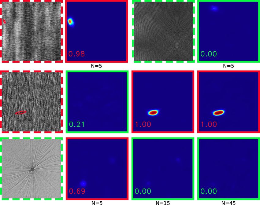
et al. [38] applied a custom 11-layer network for the same           et al. [29] further used dense conditional random fields to
task. Rački et al. [27] further proposed to improve the effi-       generate foreground/background masks that act as priors on
ciency of patch-based processing from [40] with a fully con-         an object, while Bearman et al. [2] used a single-pixel point
volutional architecture and proposed a two-stage network             label of object location instead of image-tags. Ge et al. [11]
architecture with a segmentation net for pixel-wise localiza-        used a segmentation-aggregation framework learned from
tion of the error and a classification network for per-image         weakly annotated visual data and applied it to insulator de-
defect detection. In our more recent work [35], we per-              tection on power transmission lines. Others utilized class
formed an extensive study of the two-stage architecture with         activation maps (CAM) [46]. Zhu et al. [47] applied CAM
several additional improvements and showed the state-of-             for instance segmentation, while Diba et al. [9] simultane-
the-art results that outperformed others such as U-Net [28]          ously addressed image classification, object detection, and
and DeepLabv3 [6] on a real-world case of anomaly detec-             semantic segmentation, where CAM from image classifica-
tion problem. We also extended this work and presented an            tion is used in a separate cascaded network to improve the
end-to-end learning method for the two-stage approach [5],           last two tasks.
however still in a fully-supervised regime, without consid-             Class activation maps were also applied to anomaly de-
ering the task in the context of mixed or weakly supervised          tection. Lin et al. [17] addressed defect detection in LED
learning. Dong et al. [10] also used the U-Net architecture          chips using CAM from the AlexNet architecture [46] to lo-
but combined it with SVM for classification and random               calize the defects, but learning only on the image-level la-
forests for detection. Other recent approaches also explored         bels. Zhang et al. [44] extended CAM for defect localiza-
lightweight networks [41, 18, 13, 20]. Lin et al. [18] used          tion with bounding box prediction in their proposed CADN
a compact multi-scale cascade CNN termed MobileNet-v2-               model. Their model directly predicts the bounding boxes
dense for surface-defect detection while Huang et al. [13]           from category-aware heatmaps while also using knowledge
proposed an even more lightweight network using atrous               distillation to reduce the complexity of the final inference
spatial pyramid pooling (ASPP) and depthwise separable               model. However, both methods do not consider pixel-level
convolution.                                                         labels in the learning process, thus failing to utilize this in-
                                                                     formation when available.
Unsupervised learning In unsupervised learning, anno-
tations are not needed (and are not taken into account               Mixed supervision Several related approaches also con-
even when available) and features are learned from either            sidered learning with different precision of labels. Souly
reconstruction objective [15, 7], adversarial loss [12] or           et al. [33] combined fully labeled segmentation masks
similar self-supervised objective [8, 39, 45]. In unsuper-           with unlabeled images for pixel-wise semantic segmenta-
vised anomaly detection solutions, the models are usually            tion tasks. They train the model in adversarial manner
trained considering only non-anomalous image by apply-               by generating images with GAN and include any provided
ing out-of-distribution detection of anomalies as a signif-          weak, image-level labels to the discriminator in GAN that
icant deviations in features. Various methods based on               further improves the semantic segmentation. Mlynarski et
this principle were proposed, such as AnoGAN [31] and                al. [22] addressed the problem of segmenting brain tumors
its successor f-AnoGAN [30] that utilize Generative Adver-           from magnetic resonance images. They proposed to use
sarial Networks, or a deep-metric-learning-based approach            fully segmented images and combine them with weakly an-
with triplet loss that learns features of non-anomalous sam-         notated image-level information. They focus on the goal of
ples [34], or approach that transfers pre-trained discrimina-        segmenting brain tumor images, while our primary concern
tive latent embedding into a smaller network using knowl-            is image-level anomaly detection in the industrial surface-
edge transfer for out-of-distribution detection [4], termed          defect-detection domain. They also do not perform any
Uninformed Students. The latter achieved state-of-the-art            analysis of different mixtures of the weakly and fully su-
results in unsupervised anomaly detection on the MVTec               pervised learning, which is the central point of this paper.
dataset [3], which, however, only partially reflects the com-
plexity of real-world industrial examples.
                                                                     3. Anomaly detection with mixed supervision
Weakly supervised learning Various weakly supervised                    In this section, we present a deep-learning model that
deep-learning approaches have been developed in the con-             can be trained on a mixture of fully (pixel-level) and weakly
text of semantic segmentation and object detection [26, 29,          (image-level) labeled data. Learning on weakly labeled data
2, 16, 37, 36]. In early applications, convolutional neural          requires a model capable of utilizing segmentation ground-
networks were trained with image-tags using Multiple In-             truth/masks when they are available, however, it also needs
stance Learning (MIL) [26] or with constrained optimiza-             to utilize image-level, i.e. class-only, labels as well. The
tion as in Constrained CNN [25]. The approach by Seleh               proposed model is based on our previous architecture with

                                                                 3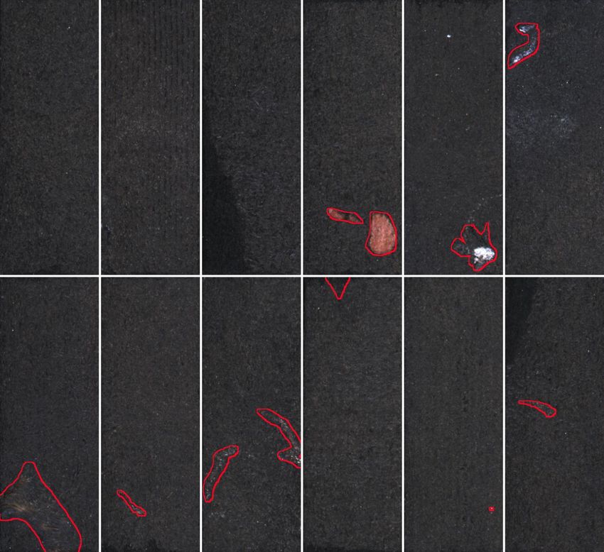
WS - Weakly Supervised Learning Learning WS
loss. The remaining parameters are: δ as an additional clas-
MS - Mixed Supervision (MS) MS
FS FS sification loss weight, γ as an indicator of the presence of
FS - Fully Supervised Learning
pixel-level annotation and λ as a balancing factor that bal-
ances the contribution of each sub-network in the final loss.
Note that λ, γ and δ do not replace the learning rate η in
SGD, but complement it. δ enables us to balance the con-
tributions of both losses, which can be on different scales
.99 since the segmentation loss is averaged over all pixels, most
of which are non-anomalous.
Segmentation Classification sub-network
We also address the problem of learning the classifica-
sub-network tion network on the initial unstable segmentation features
by learning only the segmentation at the beginning and
Figure 2: Proposed architecture with two sub-networks suit- gradually progress towards learning only the classification
able for mixed supervision. at the end. We formulate this by computing their balancing
factors as a simple linear function:
Segmentation sub-network Classification sub-network
Layer Kernel size Features Layer Kernel size Features λ = 1 − n/nep , (2)
Input: image 3/1 Input: [Sf , Sh ] 1025
2x Conv2D 5x5 32 Max-pool 2x2 1025 where n is the current-epoch index and nep is the number of
Max-pool 2x2 32 Conv2D 5x5 8 all training epochs. Without the gradual balancing of both
3x Conv2D 5x5 64 Max-pool 2x2 8
Max-pool 2x2 64 Conv2D 5x5 16 losses, the learning would in some cases result in explod-
4x Conv2D 5x5 64 Max-pool 2x2 16 ing gradients. We term the process of gradually shifting the
Max-pool 2x2 64 Conv2D (Cf ) 5x5 32
training focus from segmentation to classification as the dy-
Conv2D (Sf ) 5x5 1024 Ga (Cf ), Gm (Cf ), Ga (Sh ), Gm (Sh ) 66
Conv2D (Sh ) 1x1 1 Fully connected (Cp ) 1 namically balanced loss. Additionally, using lower δ values
can further reduce the issue of learning on the noisy seg-
Table 1: Architecture details for segmentation and classi- mentation features early on.
fication sub-networks, in which Features column represent
the number of output features. Ga and Gm represent global Using weakly labeled data The proposed end-to-end
average and max pooling operations. Outputs of the net- learning pipeline is designed to enable utilisation of the
work are a segmentation map Sh and a classification pre- weakly labeled data alongside fully labeled one. Such adop-
diction Cp . tion of mixed supervision allows us to take a full advantage
of any pixel-level labels when available, which weakly and
unsupervised methods are not capable of using. We use γ
two sub-networks [35, 5], in which the segmentation sub- from Eq. 1 to control the learning of the segmentation sub-
network utilizes fine pixel-level information and the classifi- network based on the presence of pixel-level annotation:
cation sub-network utilizes coarse image-level information.
The overall architecture with two sub-networks is depicted 1 negative image,
in Fig. 2, with the architectural details of each sub-network γ = 1 pos. image with pixel-level label, (3)
shown in Tab. 1.
0 pos. image with no pixel-level label.
3.1. Mixed supervision with end-to-end learning We disable the segmentation learning only when the pixel-
Learning from a mixture of weakly labeled and fully la- level label for an anomalous (positive) image is not avail-
beled samples is only possible when both the classification able. For non-anomalous (negative) training samples, the
and the segmentation sub-networks are trained simultane- segmentation output should always be zero for all pixels,
ously. therefore, segmentation learning can still be performed.
This allows us to treat non-anomalous training samples as
fully labeled samples and enables us to train the segmen-
End-to-end learning We combine the segmentation and
tation sub-network in the supervised mode even in the ab-
the classification losses into a single unified loss, which al-
sence of the pixel-level annotations during weakly super-
lows for a simultaneous learning in an end-to-end manner.
vised learning in the case of defect-free images.
The combined loss is defined as:
Ltotal = λ · γ · Lseg + (1 − λ) · δ · Lcls , (1) Gradient-flow adjustments We stop the gradient-flow
from the classification layers through the segmentation sub-
where Lseg and Lcls represent segmentation and classifica- network, which is required to stabilize the learning and en-
tion losses, respectively. For both, we use the cross-entropy ables training in a single end-to-end manner. During the
4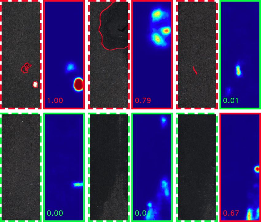
# defect
                                                                       Dataset     Subset     # images   # classes               Anotations
                                                                                                                      types
                                                                       DAGM        positive     450
                                                                                                            6           6           ellipse
                                                                         1-6       negative    3000
                                                                       DAGM        positive     600
                                                                                                            4           4           ellipse
                                                                        7-10       negative    4000
Figure 3: Segmentation loss weight mask obtained by ap-                            positive     52                                 rotated
                                                                       KSDD                                 1           1
plying distance transform algorithm on the label. Whiter                           negative     347                             bounding box
shades on the segmentation loss mask indicate pixels with                          positive     356
                                                                       KSDD2                                1          >5            fine
greater weight.                                                                    negative    2979
                                                                       Severstal   positive    4759                             fine or rotated
                                                                                                            1          >5
                                                                       Steel       negative    6666                             bounding box
initial phases of the training, the segmentation sub-network
does not yet produce meaningful outputs, hence, neither                       Table 2: Details of the the evaluation datasets.
does the classification sub-network, therefore, error gra-
dients back-propagating from the classification layers can
negatively affect the segmentation part. We propose to com-           tive pixel normalized by the maximum distance value
pletely stop those gradients, thus preventing the classifica-         within the ground-truth region and Ω(x) is a scaling func-
tion sub-network from changing the segmentation layers.               tion that converts the relative distance value into the weight
We achieve this by stopping the error back-propagation at             for the loss. In general, the scaling function Ω(x) can be
two points that connect segmentation and classification net-          defined differently depending on the defect and annotation
works. The primary point is the use of segmentation fea-              type, however, we have found that a simple power function
tures in the classification network. This is depicted by bot-         provides enough flexibility for different defect types:
tom diode symbol in Fig. 2. The second point, at which we                                     Ω(x) = wpos · xp ,                              (5)
stop error gradients is the max/avg-pooling shortcut used by
the classification sub-network. This is depicted with the top         where p controls the rate of decreasing the pixel importance
diode symbol in Fig 2. Those shortcuts utilize the segmenta-          as it gets further away from the center, while wpos is an ad-
tion sub-network’s output map to speed-up the classification          ditional scalar weight for all positive pixels. We have often
learning. Propagating gradients back through them would               found p = 1 or p = 2 as best performing, depending on
add error gradients to the segmentation’s output map, how-            the annotation type. Examples of a segmentation mask and
ever, this is unnecessary due to the already available pixel-         weights are depicted in Fig. 3. Note, that weights for nega-
level ground-truth for those features. Without gradient-flow          tively labeled pixels remain 1.
adjustments, we observed a drop in performance in fully su-
pervised scenario and greater instabilities during the train-         4. Experimental setup
ing in weak and mixed supervision.                                       In this section, we detail the datasets and the perfor-
3.2. Considering spatial label uncertainty                            mance metrics used to evaluate the proposed method as well
                                                                      as provide additional implementation details.
    When only approximate, region-based labels are avail-
able, such as shown in Fig. 3, we propose to consider dif-            4.1. Datasets
ferent pixels of the annotated defective regions differently.             We performed an extensive evaluation of the proposed
In particular, more attention is given to the center of the an-       method on four benchmark datasets. The summary of in-
notated regions and less to the outer parts. This alleviates          dividual datasets is shown in Tab. 2, while additional de-
the ambiguity arising at the edges of the defects where it            tails are provided below. A couple of images from all four
is very uncertain whether the defect is present or not. This          datasets are presented in Figs. 4, 5, 7a, 7b and 7c.
is implemented by weighting the segmentation loss accord-
ingly. We weight the influence of each pixel at positive la-
                                                                      DAGM The DAGM [40] dataset is a well-known bench-
bels in accordance with its distance to the nearest negatively
                                                                      mark dataset for surface-defect detection. It contains
labelled pixel by using the distance transform algorithm.
                                                                      grayscale images of ten different computer-generated sur-
    We formulate weighting of the positive pixels as:
                                                                      faces and various defects, such as scratches or spots. Each
                                                                      surface is treated as a binary-classification problem. Ini-

                               D(pix)
          Lseg (pix) = Ω                    · L̂(pix),      (4)       tially, six classes were presented while four additional ones
                            D(pixmax )
                                                                      were introduced later; consequently, some related methods
where L̂(pix) is the original loss of the pixel,                      report results only on the first six classes, while others re-
D(pix)/D(pixmax ) is the distance to the nearest nega-                port on all ten of them.

                                                                  5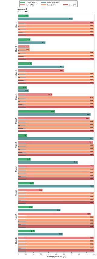
KolektorSDD The KolektorSDD [35] dataset contains
grayscale images of a real-world production item; many of
them contain visible surface cracks. Due to the small sam-
ple size, the images are split into three folds as in [35], while
final results are reported as an average of three-fold cross
validation.

KolektorSDD2 Since the above mentioned datasets have
been practically solved, and there is a huge need for
real-world, reliable, complex and well annotated surface-
detection datasets that would enable a fair comparison be-
tween different approaches, we compiled a novel dataset
Kolektor Surface-Defect Dataset 2, abbreviated as Kolek-
torSDD21 . The dataset is constructed from color images of
defective production items, captured with a visual inspec-
tion system, that were provided and partially annotated by
our industrial partner Kolektor Group d.o.o. Images for the
proposed dataset were captured in a controlled environment
and are of similar size, approximately 230 pixels wide and
630 pixels high. The dataset is split into the train and the            Figure 4: Examples of training images from KolektorSDD2
test subsets, with 2085 negative and 246 positive samples               dataset with pixel-wise annotations shown in red-overlay re-
in the train, and 894 negative and 110 positive samples in              gion.
the test subset. Defects are annotated with fine-grained seg-
mentation masks and vary in shape, size and color, ranging
from small scratches and minor spots to large surface im-               erature, to enable a fair comparison of the proposed method
perfections. Several images from this dataset are shown in              with related approaches.
Fig. 4.
                                                                        4.3. Implementation details
                                                                           The proposed architecture is implemented2 in PyTorch
Severstal Steel defect dataset The Severstal Steel de-
                                                                        framework. In all experiments, the network is trained with
fect dataset [1] is significantly larger than the other three
                                                                        stochastic gradient descent, with no momentum and with no
datasets, containing 12,568 grayscale images in 4 classes,
                                                                        weight decay. For all experiments, we disable the gradient
with various kinds of defects. We use only a subset of the
                                                                        flow from classification network to segmentation network
dataset in our evaluation. In particular, we use all nega-
                                                                        and employ loss weighting for positive pixels. We enable
tive images but consider only positive images with the most
                                                                        dynamically balanced loss for all cases with mixed super-
common defect class present in the image (class 3). The de-
                                                                        vision and fully supervised learning, but disable it when
fects are very diverse in size, shape and appearance, ranging
                                                                        only weak labels are used. Since pixel-level labels are never
from scratches and dents to excess material. Although the
                                                                        available in weakly supervised case, it has proven more use-
dataset is fairly large and diverse, some defects are quite
                                                                        ful to immediately start learning classification layers instead
ambiguous and may not be properly annotated as observed
                                                                        of delaying it with the gradual increase of λ. To account
in the third example in Fig. 7c.
                                                                        for the unbalanced datasets, we employ undersampling of
4.2. Performance metrics                                                negative samples, in each training epoch we sample a selec-
                                                                        tion of negative samples of equal size as the positive sub-
   In all experiments, we focus on evaluating per-image                 set. We also ensure that over the course of learning, all
classification metrics, which are the most relevant metrics in          negative images are used approximately as often. We also
the industrial quality control, since they decide whether to            apply morphological dilation to the annotations in datasets
keep or discard the inspected items. In particular, we mostly           where they are narrow and small in order to enlarge the la-
measure the performance in terms of the average precision               bel and facilitate distance-transform weighting. This has
(AP), which is calculated as the area under the precision-              often proven better than using narrow annotations, as small
recall curve. For the DAGM dataset, we also report several              defects can be difficult to precisely annotate, and, for some
other metrics that are used to report the results in related lit-       types of defects, the boundary between the defect and the
  1 The dataset is publicly available at https://www.vicos.si/            2 Implementation is available on github: https://github.com/

Downloads/KolektorSDD2                                                  vicoslab/mixed-segdec-net-comind2021

                                                                    6
background can not be precisely defined. Furthermore, dis-          Method                 Type
                                                                                                         10 classes             6 classes
tance transform assigns very small weights to the pixels                                          AP     AUC    F1     CA     CA     mAcc
near the edge of defects, thus dilating the annotations in-         f-AnoGAN [32]          US     19.5   57.5   27.8   79.7   81.7    54.6
creases the weights for those pixels.                               Uninf. stud. [4]       US     66.8   86.4   67.1   84.3   79.3    78.5
                                                                    Staar [34]             US      -     83.0    -      -      -       -

4.4. Training and inference time                                    CADN-W18 [44]          WS      -      -     63.2   86.2    -       -
                                                                    CADN-W18(KD)           WS      -      -     65.8   87.6    -       -
                                                                    CADN-W32 [44]          WS      -      -     69.0   89.1    -       -
    The proposed method is capable of real-time detection,          Ours (N=0)             WS     74.0   86.1   74.6   89.7   85.4    81.4
achieving 57 fps on 512 × 512 images (DAGM), 23 fps
                                                                    Ours (N=5)             MS     91.5   94.9   92.3   92.9   88.1    91.6
on 512 × 1408 images (KSDD), 85 fps on 232 × 640 im-                Ours (N=15)            MS     100    100    100    100    100     100
ages (KSDD2) and 36 fps on 1600 × 256 images (Severstal             Ours (N=45)            MS     100    100    100    100    100     100
Steel), running on a single Nvidia RTX2080Ti GPU. The               Ours (N=Nall )         FS     100    100    100    100    100     100
training time depends on the dataset size. In our experi-           Kim [14]               FS      -      -      -      -      -      99.9
                                                                    Rački [27]            FS      -     99.6    -     99.6   99.2    99.4
ments, training a model on DAGM took 35 minutes (7 or               Weimer [40]            FS      -      -      -      -      -      99.2
10 classes), on Severstal Steel (Nall = 3000) it took 460           Lin [18]               FS      -     99.0    -      -      -      99.8
                                                                    Wang [38]              FS      -      -      -      -     99.8    99.4
minutes, while for KSDD2 and KSDD (for a single fold) it
                                                                    Huang [13]             FS      -      -      -      -      -      99.8
took 15 and 32 minutes respectively.                                Liu [20] (Nall =20%)   FS      -      -      -      -     99.9     -

4.5. Related methods                                                Table 3: Comparison with related work on the DAGM
    We compare our approach against several related meth-           dataset. For AP, AUC, F1-measure and classification ac-
ods that have reported their results on DAGM [34, 44, 14,           curacy (CA), the results are averaged over all 10 classes,
27, 40, 18, 38, 13, 20] and KolektorSDD [10, 35, 19] in             whereas for (second) CA and mAcc=(TPR+TNR)/2, they
the literature. Additionally, we evaluate two state-of-the-         are averaged only over the first 6 classes for comparison
art unsupervised methods that we apply to all four datasets.        with the related work that report results only in terms of
Below, we provide more details on the implementation of             those metrics.
the two unsupervised methods.

                                                                    5. Evaluation results
Uninformed students Since the code for Uninformed-
students [4] is not publicly available, we implemented our             In this section, we present the results of the extensive
own version, which attains results comparable to the ones           evaluation of the proposed method on several industrial
reported in the literature. We additionally opted to use            quality-control problems. We first present the evaluation
a per-image defect score for classification similar to [23],        on the DAGM dataset for comparison to different related
which slightly improved results compared to the original            works, and then present results on KolektorSDD, Kolek-
implementation. For each image, we performed a 21 × 21              torSDD2 and Severstal steel, all of which represent prac-
pixel average pooling with stride = 1, to obtain patch              tical surface-anomaly detection problems taken from real-
scores, and then calculated the final image score as s =            world industrial cases. Finally, we present a detailed abla-
max(patch)/(1+avg(pixel)), i.e.   we took maximum patch             tion study that analyses the performance of individual com-
score divided by average pixel score plus one. This in-             ponents in the proposed method.
creased the AP in all four datasets.                                   We simulate and evaluate different levels of supervision
                                                                    by varying the number of positive (i.e., anomalous) training
f-AnoGAN We used publicly the available TensorFlow                  samples for which we have available pixel-wise segmenta-
implementation of f-AnoGAN [32]. In all experiments,                tion masks (i.e, the number of segmented anomalous images
we extracted 500 patches per image for training, with each          N used):
patch 64 × 64 pixels in size. In inference, a patch size of
64 × 64 pixels was extracted and classified for every pixel           i) weak supervision, with only image-level labels for all
location, which resulted in a heatmap of the same size as the            images (i.e., N = 0),
original image. For scoring, we used the distance between
the reconstructed image and the original image as well as             ii) mixed supervision, with image-level labels for all im-
between the discriminator features of the reconstructed and               ages but also pixel-level labels only for a subset of
the original image. A mean squared error was used to mea-                 anomalous images (i.e., 0 < N < Nall ), and
sure both distances. We also opted to use normalization of
the scoring similar to [23], which slightly improved results         iii) full supervision, with image-level and pixel-level la-
on noisy outputs.                                                         bels for all anomalous images (i.e., N = Nall ).

                                                                7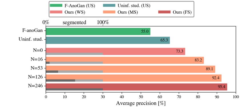
Figure 5: Examples of segmentation outputs and scores
from the proposed method on the DAGM dataset. Number
of fully labeled samples is marked with N . Border colour
indicates presence (red) or absence (green) of defects, with
dashed border around ground-truth images and solid bor-
der around predictions. The detection score that represents
the probability of the defect is indicated in the bottom left
corner.

Although we limit the number of images with the segmen-
tation mask, we always use data with the image-level label,
i.e. weak label that only indicates whether the anomaly is
present in the sample or not.

5.1. DAGM
   We first performed evaluation on the DAGM dataset.
We consider the number of positive segmented samples
N = {0, 5, 15, 45, Nall }, and use only image-level labels
for the remaining training images. In all cases, we trained
for nep = 70 epochs, with the learning rate η = 0.05, batch
size bs = 1, δ = 1, wpos = 10 and p = 1. We dilated
segmentation masks with 7 × 7 kernel.
   In Fig. 6, we show AP for all 10 classes of the dataset.
For each class, we show AP of both unsupervised methods
and of our model for all different values of N . On the bot-
tom left part of each bar, we also indicate the percentage of
the positive samples for which we used pixel-level labels,
N/Nall , which are encoded as proportions of dark and light

gray bars.
   The proposed method achieves AP of over 90% for 6
classes even with N = 0 and, on average, achieves 7.2 per-
centage points higher AP than the current state-of-the-art
unsupervised approach. Introducing only five pixel-level la-
bels allows the method to achieve 100% detection rate on 8
classes and raises the average AP to 91.5%. Finally, the
                                                                    Figure 6: Results on the DAGM dataset in terms of average
                                                                    precision (AP).
                                                                8
method achieves 100% detection rate on all 10 classes with
only 15 pixel-level labels, thus outperforming other fully
supervised approaches while having less than a quarter of
positive samples with pixel-level labels. Several examples
of detection are depicted in Fig. 5.
In Tab. 3, we compare the proposed method with a num-
ber of other approaches. We report CA and mAcc =
T P R+T N R/2 metrics averaged over the first six classes since
the related methods that use those metrics report results only
on the first six classes. Other metrics are averaged over
all 10 classes. The proposed method outperforms all other
weakly supervised and unsupervised approaches shown at
the top of the table and also all fully supervised methods
shown at the bottom of the table. Moreover, 100% detec-
tion rate can be achieved in mixed supervision with only 15
fully annotated pixel-level samples. This points to superior
performance and flexibility when allowing for mixed super-
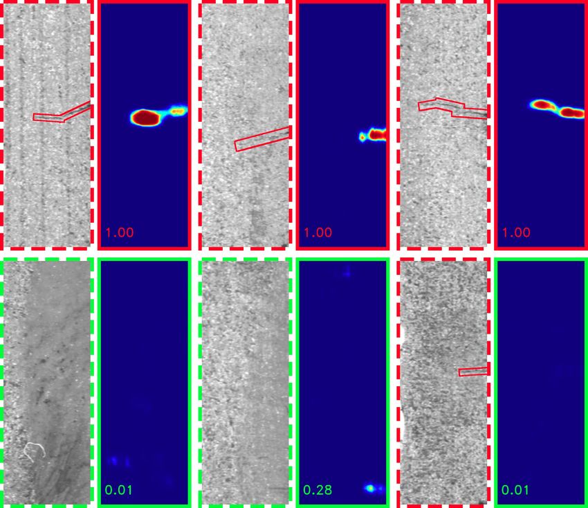
vision. (a) KolektorSDD, N = 5
5.2. KolektorSDD
On KolektorSDD dataset, we varied the number of
segmented positive samples N = {0, 5, 10, 15, 20, Nall },
where Nall = 33 and report the performance in terms of
the average precision (AP). Identical hyper-parameters were
used for all mixed and fully supervised runs, with nep = 50,
η = 1, bs = 1, δ = 0.01, wpos = 1 and p = 2, whereas
we increased δ to 1 and decreased η to 0.01 for run with
no pixel-level annotations. We dilated segmentation masks
with 7 × 7 kernel.
In the Fig. ??, we show AP for various numbers of seg-
mented positive samples. Without any segmented posi-
tive samples, our proposed approach already achieves AP
of 93.4% and significantly outperforms the current state-
of-the-art unsupervised methods that do not (and can not)
use any pixel-wise information, by roughly doubling their
results. When only 5 segmented samples are added, the (b) KolektorSDD2, N = Nall
AP drastically increases to 99.1% and approaches fairly
close to that of the fully supervised scenario. This demon-
strates well that the full annotation is often not needed for
all images and only a few annotated images are enough to
achieve respectable results. In this case, less than 15% of
images needed to be annotated, which can significantly re-
duce the annotation cost with almost no classification loss.
When using all fully labeled samples the proposed approach
achieves 100% detection rate. Several examples of defec-
tions are depicted in Fig. 7a.
5.3. KolektorSDD2
Next, we evaluate our approach on the newly proposed
KolektorSDD2 dataset. We used identical hyper-parameters
for all experiments, nep = 50, η = 0.01, bs = 1, δ = 1, (c) Severstal Steel, N = Nall = 1500
wpos = 3 and p = 2. Since the segmentation mask are very
fine, we used a larger, 15 × 15 kernel for dilation. Figure 7: Examples of detections from (a) KolektorSDD,
(b) KolektorSDD2 and (c) Severstal Steel defect dataset.
9full advantage of all the information about the samples that
it is presented with. Several examples of detections are de-
picted in Fig. 7b.
5.4. Severstal Steel defect dataset
Lastly, we evaluate the proposed method on Sever-
stal Steel defect dataset. Since this is a large dataset,
we also vary the overall number of positive training im-
ages available. We used Nall = {300, 750, 1500, 3000}
positive samples, and then for each case used N =
Figure 8: Results on the KolektorSDD2 dataset in terms of {0, 10, 50, 150, 300}, as well as N = {750, 1500, 3000},
average precision (AP). where N ≤ Nall that were segmented with pixel-wise ac-
curacy. We used all negative samples regardless of used
N and Nall . We trained for nep = {90, 80, 60, 40} when
Nall = {300, 750, 1500, 3000}, respectively, and used η =
0.1, bs = 10, δ = 0.1, wpos = 1 and p = 2.
Fig. 9, shows AP for all Nall and N . Bars are grouped
according to the Nall , with the labels showing the num-
ber of segmented positive samples and the number of pos-
itive samples without pixel-level labels. We observe that
the proposed model is capable of learning from only image-
level labeled samples, where it achieves AP of 90.3%,
91.6%, 92.5% and 94.1% for N = 0 and Nall =
{300, 750, 1500, 3000}. Note that with the positive set that
is 10 times larger, the AP only increases for 3.8 percentage
points (from 90.3% to 94.1%), pointing to a logarithmic in-
crease in performance with the increase of the number of
the positive samples. With the introduction of the pixel-
level labels, the overall performance increases significantly,
particularly for experiments with smaller Nall .
In the case of Nall = 300, the AP increases from 90.3%
to 94.2% when only 50 pixel-wise labels were added and
surpasses the AP achieved when using 3000 positive sam-
ples with image-level labels only. Furthermore, we can ob-
tain similar results by using 3000 positive samples with only
150 pixel-level labels as with using 300 positive samples
with pixel-level labels. Several examples of detections are
depicted in Fig. 7c.
Figure 9: Results of evaluation on the Severstal steel defect
database. The number of f ully + weakly labeled positive 5.5. Ablation study
samples are shown as labels to the left of the bars. Finally, we evaluate the impact of the individual compo-
nents, namely the dynamically balanced loss, the gradient-
flow adjustment and the distance transform, in the pro-
Results obtained on this challenging dataset are pre- posed model. We perform the ablation study on the DAGM,
sented in Fig. 8, where AP for all values of N are shown. KolektorSDD, and Severstal Steel Defect datasets, however,
Even without any pixel-level labels, the proposed approach for the later we use only a subset of images to reduce the
outperforms current state-of-the-art unsupervised methods training time, we used 1,000 positive and negative samples
and achieves AP of 73.3%. When 16 segmented samples are for training and the same amount for testing, we trained for
introduced, AP increases significantly to 83.2% and keeps 50 epochs.
increasing steadily with the introduction of additional pixel- We report the performance by gradually enabling in-
level labels, reaching 95.4% when N = Nall . This demon- dividual components, and by disabling a specific compo-
strates that the proposed method scales well with the intro- nent while leaving all the remaining ones enabled. Re-
duction of segmented samples and is capable of taking the sults are reported in Tab. 4. The results indicate that on
10all three datasets the worst performance is achieved with- 6. Conclusion
out any component enabled while the best performance is
achieved with all three components used. In the latter case, In this paper, we presented a deep-learning model for
the proposed model is able to completely solve the DAGM surface-anomaly detection using mixed supervision. We
and KolektorSDD datasets while achieving AP of 98.74% proposed an architecture with two sub-networks: the seg-
on Severstal Steel dataset. The second part of Tab. 4 also mentation sub-network that learns from pixel-level labels
demonstrates the importance of each component for weakly and the classification sub-network that learns from weak,
supervised learning and for mixed supervision. In both image-level labels. Combining both sub-networks allowed
cases, the best result on all three datasets is achieved only for mixing of fully and weakly labeled data to achieve
with all components enabled. Note that for weakly super- the best result with minimal annotation effort. To accom-
vised learning, we did not have any pixel-level annotations plish this, we proposed a unified network with end-to-end
and, therefore, could not apply the distance transform. We learning and enabled handling of coarse pixel-level labels.
describe the contribution of each component to the overall We demonstrated that the proposed model outperforms the
improvements in more details below. existing state-of-the-art anomaly-detection models in both
fully supervised mode and in weakly supervised mode. The
network can be applied in either weakly supervised or fully
Dynamically balanced loss Enabling only dynamic bal- supervised settings, or in a mixture of both, depending on
ancing of losses with gradual inclusion of classification net- the availability of annotations. The mixture of both an-
work already provides a boost of the performance in all notation types has resulted in performance competitive to
three datasets. In fully supervised learning, the dynamically fully supervised mode while requiring significantly fewer
balanced loss improves AP by 1.08 percentage points in and less complex annotations. We have demonstrated this
DAGM (from 89.02% to 90.10%), by 0.23 points in Kolek- on three existing industrial dataset: DAGM, KolektorSDD
torSDD (from 99.77% to 100.00%) and by 1.68 points and Severstal Steel Defect, and have additionally proposed
in Severstal Steel (95.36% to 97.04%). Similar improve- KolektorSDD2 that represents a real-world industrial prob-
ments can also be observed in mixed supervision, with 4.44, lem with several defect types spread over 3000 images.
0.75 and 1.99 percentage points improvements for DAGM, Two important conclusions can be drawn from the re-
KolektorSDD and Severstal Steel. sults. First, using a large number of only weakly labeled
data has proven to be more important than using a 10-fold
Gradient-flow adjustment The gradient-flow adjustment smaller set of fully labelled samples. In cases, such as exist-
has proven to be equally important as the dynamically bal- ing industrial production control where weakly labeled data
anced loss. Both improvements naturally result in a similar can be obtained at no cost, it is much less costly to use a
performance in KolektorSDD and Severstal Steel since they large set of weakly labeled data without sacrificing the per-
both prevent unstable segmentation features to significantly formance. However, as a second conclusion, we observed
affect learning of the classification layers in the early stages. that a significant performance boost is often obtained when
However, enabling both improvements is more robust as it adding just 5–10% of fully-labeled data, resulting in almost
eliminates the convergence issues while also improving re- the same performance as using all fully-labeled data. This
sults on all three datasets, especially for DAGM, in which realization can considerably reduce the time and cost of data
100% detection rate can be achieved for fully supervised annotation in many industrial applications.
learning and AP of 95.37% for mixed supervision. On the
other hand, it has also proven better to use only gradient- Acknowledgments
flow adjustment in weak supervision and to completely dis-
able dynamically balanced loss, since in this case segmen- This work was in part supported by the ARRS research
tation loss is not present. project J2-9433 (DIVID) and research programme P2-0214.
We would also like to thank Kolektor Group d.o.o. for
Spatial label uncertainty Lastly, enabling the distance providing images and initial annotations used in Kolek-
transform as weights for the positive pixels pushes perfor- torSDD2 dataset.
mance on KolektorSDD to 100% detection rate, therefore
completely solving KolektorSDD and DAGM in fully su- References
pervised mode. It also improves AP on Severstal Steel [1] Severstal: Steel Defect Detection on Kaggle Challenge. 2, 6
dataset from 98.24% to 98.74%. Moreover, distance trans- [2] A. Bearman, V. Ferrari, and O. Russakovsky. What’s the
form is even more important in mixed supervision where point : Semantic segmentation with point supervision. In
it enables 100% detection rate with only 25% of fully an- ECCV, pages 1–11, 2016. 3
notated data and using only weak labels for the remaining [3] P. Bergmann, M. Fauser, D. Sattlegger, and C. Steger.
data. MVTec AD — A Comprehensive Real-World Dataset for
11DAGM KolektorSDD Severstal Steel Dynamically Gradient-flow Distance
balanced loss adjustment transform
AP FP+FN AP FP+FN AP FP+FN
89.02 1010+45 99.77 0+1 95.36 108+121
(N=100%)
90.10 995+14 100.00 0+0 97.04 95+76 X
100.00 0+0 99.88 1+0 98.24 52+58 X X
FS
91.88 471+68 99.88 1+0 97.80 57+60 X X
99.95 2+2 99.75 1+0 98.32 73+64 X X
100.00 0+0 100.00 0+0 98.74 59+40 X X X
66.02 2497+56 99.06 2+1 94.36 136+120
(N ≈ 25%)
70.46 1775+65 99.81 2+0 96.35 113+96 X
95.37 22+56 99.10 0+2 96.88 57+105 X X
MS
91.44 837+19 99.40 1+1 92.49 183+137 X X
99.93 0+3 99.16 1+2 96.60 122+83 X X
100.00 0+0 99.10 0+2 97.73 67+64 X X X
(0%)
74.05 438+248 93.43 4+5 91.01 201+158 X N/A
WS
61.49 1947+127 93.16 3+5 90.88 247+120 X X N/A
Table 4: Performance of individual components on three datasets by gradually including each one for fully supervised (FS),
mixed supervision (MS), and weakly supervised (WS) learning. We report average precision (AP) and the number of false
positives (FP) and false negatives (FN).
Unsupervised Anomaly Detection. In CVPR 2019, pages method for industrial applicable object detection. Computers
9592–9600, 2019. 3 in Industry, 121, 2020. 3
[4] P. Bergmann, M. Fauser, D. Sattlegger, and C. Steger. [12] I. Goodfellow, J. Pouget-Abadie, and M. Mirza. Genera-
Uninformed students: Student-teacher anomaly detection tive Adversarial Networks. In Neural Information Process-
with discriminative latent embeddings. In 2020 IEEE/CVF ing Systems, pages 1–9, 2014. 3
Conference on Computer Vision and Pattern Recognition [13] Y. Huang, C. Qiu, X. Wang, S. Wang, and K. Yuan. A com-
(CVPR), pages 4182–4191, 2020. 2, 3, 7 pact convolutional neural network for surface defect inspec-
[5] J. Božič, D. Tabernik, and D. Skočaj. End-to-end training tion. Sensors, 20(7), 2020. 2, 3, 7
of a two-stage neural network for defect detection. In 2020 [14] S. Kim, W. Kim, Y. Noh, and F. C. Park. Transfer learning
25th International Conference on Pattern Recognition, pages for automated optical inspection. In 2017 International Joint
5619–5626, 2020. 3, 4 Conference on Neural Networks (IJCNN), pages 2517–2524,
[6] L.-C. Chen, G. Papandreou, F. Schroff, and H. Adam. Re- 2017. 2, 7
thinking Atrous Convolution for Semantic Image Segmenta- [15] D. P. Kingma, D. J. Rezende, S. Mohamed, and M. Welling.
tion. CoRR, abs/1706.05587, 2017. 3 Semi-Supervised Learning with Deep Generative Models. In
[7] X. Chen, D. P. Kingma, T. Salimans, Y. Duan, P. Dhariwal, Neural Information Processing Systems, pages 1–9, 2014. 3
J. Schulman, I. Sutskever, and P. Abbeel. Variational Lossy [16] Q. Li, A. Arnab, and P. H. Torr. Weakly- and semi-supervised
Autoencoder. In International Conference on Learning Rep- panoptic segmentation. Lecture Notes in Computer Science,
resentations, pages 1–17, 2017. 3 11219 LNCS:106–124, 2018. 3
[8] I. Croitoru, S.-V. Bogolin, and M. Leordeanu. Unsupervised [17] H. Lin, B. Li, X. Wang, Y. Shu, and S. Niu. Automated de-
learning from video to detect foreground objects in single fect inspection of LED chip using deep convolutional neural
images. In International Conference on Computer Vision, network. Journal of Intelligent Manufacturing, pages 1–10,
pages 4335–4343, 2017. 3 2018. 1, 2, 3
[9] A. Diba, V. Sharma, A. Pazandeh, H. Pirsiavash, and L. Van [18] Z. Lin, H. Ye, B. Zhan, and X. Huang. An efficient network
Gool. Weakly supervised cascaded convolutional networks. for surface defect detection. Applied Sciences, 10:6085, 09
Proceedings - 30th IEEE Conference on Computer Vision 2020. 2, 3, 7
and Pattern Recognition, CVPR 2017, 2017-Janua:5131– [19] G. Liu, N. Yang, L. Guo, S. Guo, and Z. Chen. A one-stage
5139, 2017. 3 approach for surface anomaly detection with background
[10] X. Dong, C. J. Taylor, and T. F. Cootes. Defect Detection and suppression strategies. Sensors, 20:1829, 03 2020. 7
Classification by Training a Generic Convolutional Neural [20] Y. Liu, Y. Yuan, C. Balta, and J. Liu. A light-weight deep-
Network Encoder. IEEE Transactions on Signal Processing, learning model with multi-scale features for steel surface de-
68(1):6055–6069, 2020. 3, 7 fect classification. Materials, 13(20):1–13, 2020. 3, 7
[11] C. Ge, J. Wang, J. Wang, Q. Qi, H. Sun, and J. Liao. Towards [21] J. Masci, U. Meier, D. Ciresan, J. Schmidhuber, and
automatic visual inspection: A weakly supervised learning G. Fricout. Steel defect classification with Max-Pooling
12Convolutional Neural Networks. In Proceedings of the In- [36] F. Wan, C. Liu, W. Ke, X. Ji, J. Jiao, and Q. Ye. C-MIL: Con-
ternational Joint Conference on Neural Networks, pages 1– tinuation Multiple Instance Learning for Weakly Supervised
6, 06 2012. 2 Object Detection. In Computer Vision and Pattern Recogni-
[22] P. Mlynarski, H. Delingette, A. Criminisi, and N. Ayache. tion, volume 1, pages 2199–2208, 2019. 3
Deep learning with mixed supervision for brain tumor seg- [37] F. Wan, P. Wei, J. Jiao, Z. Han, and Q. Ye. Min-Entropy
mentation. Journal of Medical Imaging, 6:034002, 2019. 2, Latent Model for Weakly Supervised Object Detection. Pro-
3 ceedings of the IEEE Computer Society Conference on Com-
[23] T.-N. Nguyen and J. Meunier. Anomaly detection in video puter Vision and Pattern Recognition, pages 1297–1306,
sequence with appearance-motion correspondence. In 2019 2018. 3
IEEE/CVF International Conference on Computer Vision [38] T. Wang, Y. Chen, M. Qiao, and H. Snoussi. A fast and
(ICCV), pages 1273–1283, 10 2019. 7 robust convolutional neural network-based defect detection
[24] D. M. Onchis and G.-r. Gillich. Stable and explainable deep model in product quality control. The International Journal
learning damage prediction for prismatic cantilever steel of Advanced Manufacturing Technology, 94(9):3465–3471,
beam. Computers in Industry, 125:103359, 2021. 1, 2 Feb 2018. 2, 3, 7
[25] D. Pathak, P. Krähenbühl, and T. Darrell. Constrained Con- [39] X. Wang, K. He, and A. Gupta. Transitive Invariance for
volutional Neural Networks for Weakly Supervised Segmen- Self-supervised Visual Representation Learning. In Interna-
tation Multi-class Image Segmentation. In International tional Conference on Computer Vision, 2017. 3
Conference on Computer Vision, pages 1–28, 2015. 3 [40] D. Weimer, B. Scholz-Reiter, and M. Shpitalni. Design of
[26] D. Pathak, E. Shelhamer, J. Long, and T. Darrell. Fully Con- deep convolutional neural network architectures for auto-
volutional Multi-Class Multiple Instance Learning. In In- mated feature extraction in industrial inspection. CIRP An-
ternational Conference on Learning Representations Work- nals - Manufacturing Technology, 65(1):417–420, 2016. 1,
shop, number 1, pages 1–4, 2015. 3 2, 3, 5, 7
[27] D. Rački, D. Tomaževič, and D. Skočaj. A compact convolu- [41] Y. Yang, R. Yang, L. Pan, J. Ma, Y. Zhu, T. Diao, and
tional neural network for textured surface anomaly detection. L. Zhang. A lightweight deep learning algorithm for inspec-
In IEEE Winter Conference on Applications of Computer Vi- tion of laser welding defects on safety vent of power battery.
sion, pages 1331–1339, 2018. 2, 3, 7 Computers in Industry, 123:103306, 2020. 1, 3
[28] O. Ronneberger, P. Fischer, and T. Brox. U-Net: Convo- [42] J. Yu, X. Zheng, and J. Liu. Stacked convolutional sparse
lutional Networks for Biomedical Image Segmentation. In denoising auto-encoder for identification of defect patterns in
Medical Image Computing and Computer-Assisted Interven- semiconductor wafer map. Computers in Industry, 109:121–
tion – MICCAI 2015, pages 234–241, 2015. 3 133, 2019. 1, 2
[29] F. Saleh, M. S. A. Akbarian, M. Salzmann, L. Petersson, [43] V. Zavrtanik, M. Kristan, and D. Skočaj. Reconstruction by
S. Gould, and J. M. Alvarez. Built-in foreground/background inpainting for visual anomaly detection. Pattern Recogni-
prior for weakly-supervised semantic segmentation. Lecture tion, 112:107706, 2021. 2
Notes in Computer Science, 9912 LNCS:413–432, 2016. 3 [44] J. Zhang, H. Su, W. Zou, X. Gong, Z. Zhang, and F. Shen.
[30] T. Schlegl, P. Seeböck, S. M. Waldstein, G. Langs, and Cadn: A weakly supervised learning-based category-aware
U. Schmidt-Erfurth. f-AnoGAN: Fast unsupervised anomaly object detection network for surface defect detection. Pattern
detection with generative adversarial networks. Medical Im- Recognition, 109:107571, 2021. 2, 3, 7
age Analysis, 54:30–44, 2019. 3 [45] R. Zhang, P. Isola, and A. A. Efros. Split-Brain Autoen-
[31] T. Schlegl, P. Seeböck, S. M. Waldstein, U. Schmidt-Erfurth, coders: Unsupervised Learning by Cross-Channel Predic-
and G. Langs. Unsupervised anomaly detection with genera- tion. In Computer Vision and Pattern Recognition, pages
tive adversarial networks to guide marker discovery. Lecture 645–654, 07 2017. 3
Notes in Computer Science, 10265 LNCS:146–147, 2017. 3 [46] B. Zhou, A. Khosla, A. Lapedriza, A. Oliva, and A. Tor-
[32] T. Schlegl, P. Seeböck, S. M. Waldstein, G. Langs, and ralba. Learning Deep Features for Discriminative Localiza-
U. Schmidt-Erfurth. f-anogan: Fast unsupervised anomaly tion. In Computer Vision and Pattern Recognition, pages
detection with generative adversarial networks. Medical Im- 2921–2929, 2016. 3
age Analysis, 54:30 – 44, 2019. 7 [47] Y. Zhu, Y. Zhou, H. Xu, Q. Ye, D. Doermann, and J. Jiao.
[33] N. Souly, C. Spampinato, and M. Shah. Semi Supervised Learning Instance Activation Maps for Weakly Supervised
Semantic Segmentation Using Generative Adversarial Net- Instance Segmentation. IEEE Conference on Computer Vi-
work. In International Conference on Computer Vision, sion and Pattern Recognition (CVPR), pages 3116–3125,
pages 5688–5696, 2017. 2, 3 2019. 2, 3
[34] B. Staar, M. Lütjen, and M. Freitag. Anomaly detection with
convolutional neural networks for industrial surface inspec-
tion. Procedia CIRP, 79:484 – 489, 2019. 2, 3, 7
[35] D. Tabernik, S. Šela, J. Skvarč, and D. Skočaj.
Segmentation-based deep-learning approach for surface-
defect detection. Journal of Intelligent Manufacturing, pages
1–18, 2019. 1, 2, 3, 4, 6, 7
13You can also read