Modeling and imaging based on acoustic or seismic waves: a combination of numerical modeling, high performance computing, and big data
←
→
Page content transcription
If your browser does not render page correctly, please read the page content below

Modeling and imaging based on acoustic
  or seismic waves: a combination of
 numerical modeling, high performance
        computing, and big data
      Dimitri Komatitsch (and many others)

     Laboratoire de Mécanique et d’Acoustique
             CNRS, Marseille, France
          ITN WAVES, Marseille, France
                01 June 2017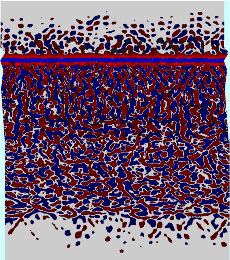
Application domains
             Different application domains of acoustic
             full waveform numerical modeling
                Earthquakes

                                 Ocean
                                 acoustics

             Non destructive testing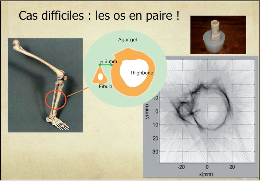
Equations of motion (solid)
Differential or strong form (e.g., finite differences):
u f
2
t
We solve the integral or weak form in the time domain:
2 3 3
w u d
t r w : d r
Μ : w rs S t w nˆ d r
2
F S
+ attenuation (memory variables)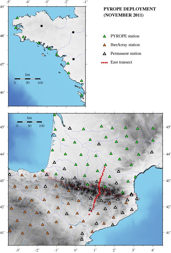
Equations of motion (fluid)
Differential or strong form in the time domain:
t v p t p v
with the adiabatic bulk modulus.
We use a scalar potential
of * displacement:
u p 2
t
The integral or weak form is:
1 1
w d2
tr 3
w d r 3
cheap (scalar potential)
natural coupling with solid
w nˆ v d r
2
F S
Spectral-Element Method Developed in Computational Fluid Dynamics (Patera 1984) Accuracy of a pseudospectral method, flexibility of a finite-element method Extended by Komatitsch and Tromp, Chaljub et al. Large curved “spectral” finite- elements with high-degree polynomial interpolation Mesh honors the main discontinuities (velocity, density) and topography Very efficient on parallel computers, no linear system to invert (diagonal mass matrix)
Finite elements High-degree pseudospectral finite elements N = 5 to 8 usually Strictly diagonal mass matrix No linear system to invert Fully explicit time scheme
Our SPECFEM3D software package

            User download map

Goal: model acoustic / elastic / viscoelastic / poroelastic / seismic wave propagation in in non
      destructive testing, in ocean acoustics, in the Earth (earthquakes, oil industry)…
                   The SPECFEM3D source code is open (GNU GPL v2)

Initially Komatitsch and Vilotte at IPG Paris (France), mostly developed by Dimitri Komatitsch
 and Jeroen Tromp at Harvard University, then Caltech, Princeton (USA) and CNRS (France)
                                          since 1996.
  Improved with INRIA and University of Pau (France), ETH Zürich and University of Basel
         (Switzerland), the Barcelona Supercomputing Center (Spain), NVIDIA…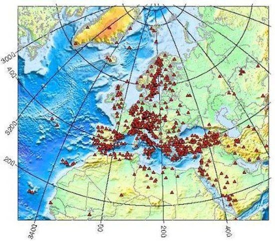
Earthquake hazard assessment
Use parallel computing to   2001 Gujarati (M 7.7) Earthquake, India
simulate earthquakes

Learn about structure of
the Earth based upon
seismic waves
(tomography)

Produce seismic hazard
maps (local/regional
scale) e.g. Los Angeles,       20,000 people killed
Tokyo, Mexico City,            167,000 injured
Seattle                        ≈ 339,000 buildings destroyed
                               783,000 buildings damaged
Earthquakes

                                          (Italy)

                                               310 casualties
                                               ~ 1000 injured
                                             ~ 26000 homeless

                         Istituto Nazionale di
                         Geofisica e Vulcanologia

Collaboration with
Emanuele Casarotti and Federica Magnoni (INGV Roma, Italy)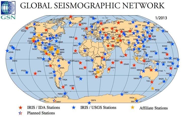
L’Aquila, Italy, April 6, 2009 (Mw = 6.2)

Location of the epicenter
(© Google Maps)             Mesh defined on the
                            JADE supercomputer
                            on April 7, 2009
GSA GSA GSA
AVZ AVZ AVZ
1D flat - max PGV 45 cm/s 1D w topo - max PGV 48 cm/s 3D - max PGV 74 cm/s
Max PGV data in the epicentral area ~ 65 cm/s
(Faenza et al., 2011)Adjoint methods for tomography
and imaging for automatic differentiation (AD, autodiff)
Problem is self-adjoint, thus no need
Theory: A. Tarantola, Talagrand and Courtier.
‘Banana-Donut’ kernels (Tony Dahlen et al., Princeton)
Close to time reversal (Mathias Fink et al.) but not identical,
thus interesting developments to do.
Idea: apply this to tomography of the full Earth
(current ANR / NSF contract with Princeton University, USA), and in acoustic
tomography: ocean acoustics, non destructive testing.Princeton, USA
L-BFGS method
t −1 −1
Iterative Gauss-Newton algorithm mk + 1 = mk + (G k G k + C m ) ∇ J (mk )
δmk
L-BFGS (Low-memory Broyden–Fletcher–Goldfarb–Shanno):
Approximate
δmk
from:
m k − 1 , m k− 2 , m k− 3 , ... , m 0
∇ J (mk − 1 ), ∇ J (m k − 2) , ... , ∇ J (m 0 )
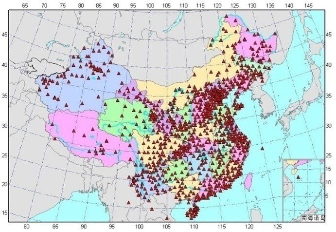
→ no need to invert or even build a big matrixRéseaux denses d’enregistrement Des réseaux denses d’enregistrement impliquent du “big data” pour la tomographie. Ceci va conduire à de bien meilleures images en tomographie et imagerie (ici, de la Terre). Cela veut dire que l’on a besoin de HPDA [web.mst.edu] (High-Performance Data Analysis) et non plus simplement de HPC (High-Performance Computing). [www.geo.uib.no] [data.earthquake.cn] [drh.edm.bosai.go.jp]
Oil industry applications TOTAL S.A.
Offshore In foothill regions
• Elastic wave propagation in complex 3D structures,
• Often fluid / solid problems: many oil fields are located offshore (deep
offshore, or shallower).
• Anisotropic rocks, geological faults, cracks, bathymetry / topography…
• Thin weathered zone / layer at the surface model dispersive surface waves."Big Data" in seismology:
[www.iris.edu]
[www.geo.uib.no] [data.earthquake.cn]
and in the oil and gas industry:
3D marine surveys can involve
5,000 shots and 50,000 receivers:
• Petabytes of data
• Need for « big data » tools
• High-Performance Data Analysis
(HPDA) rather than pure HPCProjet industriel pétrolier « OROGEN »
Imagerie Techniques
sismique d’imagerie
très haute adaptées
résolution
Les ondes sismiques venant de toute la terre éclairent et permettent
d’imager une structure géologique donnée (ici les Pyrénées).
Plus haute résolution jamais atteinte, grâce au calcul haute performance.A hybrid approach: Coupling global and
regional propagations
A hybrid technique for 3-D waveform modeling
and inversion of high frequency teleseismic
body waves
Regional propagation
3-D spherical shell
Global propagation
Spherically symmetric Earth model
S. Chevrot, V. Monteiller, D. Komatitsch & N. Fuji
Geophysical Journal International, 2014Local inversion based on coupling with teleseismic
wave propagation Monteiller et al, GJI 2013
3D mesh box
1D, 2.5D or 3D model outside
computed e.g. based on DSM, GEMINI,
AxiSEM or even SPECFEM3D_GLOBE itself
Full 3D wave propagation inside the box
at the regional scale based on spectral elements
Coupling of both methods for full waveform inversion at high frequency (down to 1 second)Synthetic full waveform inversion example
Full waveform inversion:
Adjoint tomography:
Full waveform modeling :
- Direct P wave
- Converted waves
- Reflected waves
5 L-BFGS iterations of full waveform inversion
vs. 15 iterations of adjoint tomographySynthetic full waveform inversion example
Full waveform modeling :
- Direct P wave
- Converted waves
- Reflected waves
With hierarchical frequency contentSynthetic full waveform inversion example
Full waveform modeling :
- Direct P wave
- Converted waves
- Reflected waves
Without hierarchical frequency content
not good (Pratt et al. 1998)Imaging the Pyrénées Mountains
Drastically-improved quality
of the images thanks to the
high frequencies involved
This results in a much more precise and therefore much more interesting
geological interpretation (how the Earth formed and keeps evolving)
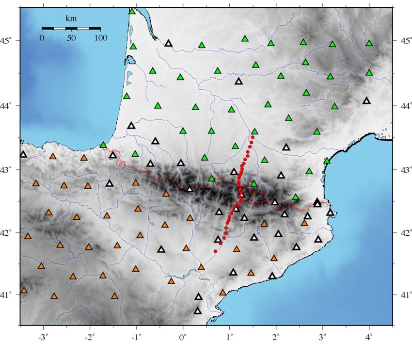
Wang et al., Geology, vol. 44, p. 475-478 (2016).The PYROPE experiment
French/Spanish initiative, supported
by the French ANR
~150 temporary + 50 permanent BB
stations
Interstation spacing ~ 60 km
Dense transects across the PyrénéesAbout the path to exaflops
Projected supercomputer performance evolution
(adapted from www.top500.org)
• End of 2018 for exaflop/s, end of 2017 for petaflop/s easily everywhere,
around 2027 for exaflop/s easily everywhere (?)
• For SPECFEM3D it is increasingly needed to perform a very large number
(thousands!) of medium-size runs (500 to 2000 cores), rather than a single,
very large grand-challenge run; this comes from solving imaging problems
iteratively rather than a single forward problem once.The path to exaflops and beyond
Nomenclature:
• petaflop/s 1015 (current, since 2009)
• exaflop/s 1018 (end of 2018)
• zettaflop/s 1021 ( 2027?)
• yottaflop/s 1024 ( 2036??)
Flop/s: number of floating-point operations
that the computer performs per second.GPU graphics cards Host Device
Grid 1
Kernel Block Block Block
1 (0, 0) (1, 0) (2, 0)
Block Block Block
(0, 1) (1, 1) (2, 1)
Grid 2
Kernel
2
NVIDIA
Block (1, 1)
Why are they so powerful for Thread Thread Thread Thread Thread
scientific computing? (0, 0) (1, 0) (2, 0) (3, 0) (4, 0)
Thread Thread Thread Thread Thread
(0, 1) (1, 1) (2, 1) (3, 1) (4, 1)
Massive lightweight Thread Thread Thread Thread Thread
multithreading.
(0, 2) (1, 2) (2, 2) (3, 2) (4, 2)
Collaboration with D. Peter (ETH Zürich), P. Messmer (NVIDIA),
D. Göddeke (Dortmund, Germany)Our PRACE European project PRACE project with INGV Roma (E. Casarotti, F. Magnoni, D. Melini, A. Michelini) + Princeton University, USA (J. Tromp) + University of Fairbanks, Alaska (C. Tape) to image the Italian lithosphere: 40 million core hours on CURIE (PRACE / TGCC, France) “IMAGINE_IT: 3D full-wave tomographic IMAGINg of the Entire ITalian lithosphere”
Projets EDF et CEA en contrôle non destructif
                                          La modélisation numérique permet d’étudier
                                        facilement différents modèles de chanfreins pour
                                               les tubes de sortie du sodium chaud.

                                           Propagation et contrôle dans du sodium liquide (avec le CEA).

                                        La modélisation numérique permet d’aller au‐delà
                                        des fonctions de diffusion usuelles, aussi d’étudier
                                              la zone interfaciale de transition (ITZ).
Propagation et contrôle dans du béton
            (avec EDF).
Non destructive testing of materials
Collaboration with Non Destructive Testing Lab in
Marseille.
Currently: Physical modeling based on diffusion functions
for objects of complex shape, cracks or multiple cavities in
concrete, metals, or composite materials. Experiments on
samples.
Very accurate calculations without homogenization can
validate (or not) these diffusion functions and extend them
beyond their domain of validity.
Reliable modeling of the “coda” part of the signal, which
contains useful information on the medium.Pour l’imagerie médicale Par Philippe Lasaygues, CNRS, mars 2014.
Exemple de projet en imagerie médicale

                                                      Image d’une paire tibia-péroné reconstruite
                                                         par FWI sur données synthétiques.

                                                              Imagerie médicale

                                    Liens avec notre équipe « Ultrasons médicaux »,
    Imagerie sismique                   qui a de très belles données + expertise.

                 Nouvelles contraintes : l’inversion doit être rapide,
faibles vitesses des ondes de cisaillement, position des récepteurs très différente.
Ocean acoustics
Numerical simulation Collaboration with Paul Cristini.
Wave propagation across an
impedance discontinuity.
Influence on interface waves.
Going beyond usual Chalk Basalt
approximations (parabolic).
Experiments performed in tanks
Experiments in known environment / setup
Experimental tanks in Marseille
Perform experimental benchmarksOcean acoustics and monitoring Numerical simulation Wave propagation across seamounts, earthquake T waves… Experiments performed in tanks Experimental tanks in Marseille Objects with a complex shape
Conclusions and future work
On modern computers, large 3D full-waveform forward modeling
problems can be solved at high resolution in the time domain for
acoustic / elastic / viscoelastic / poroelastic / seismic waves
Inverse (adjoint) tomography / imaging problems can also be
studied, although the cost is still high
Useful in different industries in addition to academia: oil and gas,
medical imaging, ocean acoustics / sonars, non destructive testing
(concrete, composite media, fractures, cracks)
Hybrid (GPU) computing is useful to solve inverse problems in
seismic wave propagation and imaging
PRACE project with INGV Roma to image the Italian lithosphere:
40 million core hours on a petaflop machine
Some future trends: high-frequency ocean acoustics, tomography of
buried objects, wavelet compressionAcknowledgements and funding This project has received funding from the European Union’s Horizon 2020 research and innovation programme under the Marie Sklodowska-Curie grant agreement No 641943.
You can also read