Modeling of negative protein-protein interactions: methods and experiments - arXiv
←
→
Page content transcription
If your browser does not render page correctly, please read the page content below
arXiv:1910.04709v1 [q-bio.MN] 10 Oct 2019

                                            Modeling of negative protein-protein
                                            interactions: methods and experiments

                                            Facoltà di Ingegneria dell’Informazione, Informatica e Statistica
                                            Corso di Laurea Magistrale in Computer Science

                                            Candidate
                                            Andrea Moscatelli
                                            ID number 1667647

                                            Thesis Advisor                                  Co-Advisor
                                            Prof. Paola Velardi                             Prof. Giovanni Stilo

                                            Academic Year 2018/2019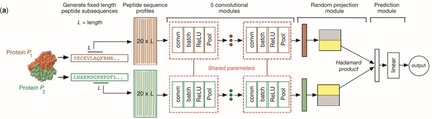
Modeling of negative protein-protein interactions: methods and experiments
Master thesis. Sapienza – University of Rome

© 2019 Andrea Moscatelli. All rights reserved

This thesis has been typeset by LATEX and the Sapthesis class.

Version: October 11, 2019
Author’s email: andrea.moscatelli95@gmail.com
ii

Acknowledgments

First, I would like to thank my thesis advisor, Professor Paola Velardi, who, with
her integrity and transparency, allowed me to grow humanly and professionally. Her
feedback, advice and suggestions were priceless.
I would also like to thank Professor Yang Yu-Liu and Professor Song (Stephen) Yi.
This work would not be as successful without their participation and contribution.
Moreover, I express my profound gratitude to my family, which unconditionally
supported me during my whole life, allowing me to achieve our results. The best is
yet to come.
Finally, I would also like to thank all my friends and colleagues, which, in various
ways, have helped me while I was completing my thesis. Thanks to Luca, which shared
with me joys, sorrows, tv series and video games. Thanks to Monti, 3 Etti and Alessio,
which backed me all the way. Thanks to Motino, which was always there for me.
And a big thanks also to all the others: Lorenzo, Irene, Alessio, Maurizio, Perna,
Martina, Mary, Giulia, Rubia, Macchietta, Flavio, Roberto, Antonio, Federica,
Giuseppe, Vicky, Marianna, Silvia, Omar, Ilaria, Jacopo.
iii

Contents

1 Introduction                                                                           1

2 Backgrounds needed                                                                     3
  2.1   Computer Science background . . . . . . . . . . . . . . . . . . . . . .          3
  2.2   Biological background . . . . . . . . . . . . . . . . . . . . . . . . . .        4

3 Datasets                                                                               8
  3.1   HuRI . . . . . . . . . . . . . . . . . . . . . . . . . . . . . . . . . . . .    10
  3.2   LIT-BM . . . . . . . . . . . . . . . . . . . . . . . . . . . . . . . . . .      11
  3.3   HQND . . . . . . . . . . . . . . . . . . . . . . . . . . . . . . . . . . .      12

4 PPIs prediction review in literature                                                  13
  4.1   Connection-based methods        . . . . . . . . . . . . . . . . . . . . . . .   14
  4.2   Protein-based methods . . . . . . . . . . . . . . . . . . . . . . . . . .       16

5 The negative interactions issue                                                       20
  5.1   Random sampling . . . . . . . . . . . . . . . . . . . . . . . . . . . .         21
  5.2   Subcellular location heuristic . . . . . . . . . . . . . . . . . . . . . .      23
  5.3   Other methods . . . . . . . . . . . . . . . . . . . . . . . . . . . . . .       24
        5.3.1   Bait-prey approach . . . . . . . . . . . . . . . . . . . . . . . .      24
        5.3.2   Negatome 2.0 . . . . . . . . . . . . . . . . . . . . . . . . . . .      25
        5.3.3   Sequence similarity and shortest paths . . . . . . . . . . . . .        27
        5.3.4   Hybrid methods . . . . . . . . . . . . . . . . . . . . . . . . .        28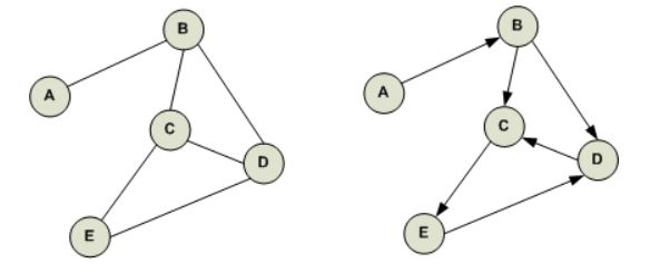
Contents                                                                               iv

6 Comparison of methods generating negative interactions                               29
  6.1   VER and MER . . . . . . . . . . . . . . . . . . . . . . . . . . . . . .        31
  6.2   VSR . . . . . . . . . . . . . . . . . . . . . . . . . . . . . . . . . . . .    36
  6.3   ATER . . . . . . . . . . . . . . . . . . . . . . . . . . . . . . . . . . .     37
  6.4   Final considerations . . . . . . . . . . . . . . . . . . . . . . . . . . .     39

7 Computational PPIs prediction                                                        40
  7.1   Features . . . . . . . . . . . . . . . . . . . . . . . . . . . . . . . . . .   42
  7.2   Models . . . . . . . . . . . . . . . . . . . . . . . . . . . . . . . . . . .   48
        7.2.1   Random Forest Classifier . . . . . . . . . . . . . . . . . . . .       49
        7.2.2   Support Vector Machine . . . . . . . . . . . . . . . . . . . . .       49
        7.2.3   Multi-layer Perceptron classifier . . . . . . . . . . . . . . . . .    50
        7.2.4   Gradient Boosting . . . . . . . . . . . . . . . . . . . . . . . .      50
        7.2.5   Convolutional Neural Networks . . . . . . . . . . . . . . . . .        51
        7.2.6   DNN-PPI . . . . . . . . . . . . . . . . . . . . . . . . . . . . .      51
        7.2.7   DPPI . . . . . . . . . . . . . . . . . . . . . . . . . . . . . . .     52
  7.3   Experiments . . . . . . . . . . . . . . . . . . . . . . . . . . . . . . . .    53
  7.4   Features’ importance . . . . . . . . . . . . . . . . . . . . . . . . . . .     60

8 PPIs extraction from biomedical literature                                           61
  8.1   Negative protein interactions detection . . . . . . . . . . . . . . . . .      62

9 Conclusions                                                                          68
  9.1   Future work . . . . . . . . . . . . . . . . . . . . . . . . . . . . . . . .    69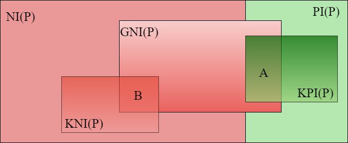
1

Chapter 1

Introduction

The interactions between proteins, also referred as protein-protein interactions
(PPIs), are of fundamental importance for the human body, and the knowledge
about their existence could provide useful insights when performing critical tasks, as
drug target developing and therapy design.
   However, the high-throughput laboratory experiments generally used to discover
new protein-protein interactions are very costly and time consuming, stressing
the need of new computational methods able to predict high-quality PPIs. These
methods have to face two main problems: (i) the very low number of PPIs already
known and (ii) the lack of high-quality negative protein-protein interactions (i.e.
proteins that are known to not interact). The former is due to the high number
of PPIs in the human body and the high cost of the PPIs detection laboratory
experiments. Instead, the latter is usually overlooked by the PPIs prediction systems,
causing a significant bias in the performances and metrics.
   This work is particularly focused on the issue regarding the absence of negative
interactions. This problem is of crucial importance since, to predict high-quality
PPIs, the computational systems have to learn from both positive and negative
instances, and, even when only positive examples are exploited in training, negative
data are still needed to evaluate performances in an appropriate manner.
   Our results show that some methods for generating reliable negative instances
are more effective than others and that the performances reported by the PPIs
prediction systems in literature are usually overestimated, mainly because of the
2

negative interactions used in the training and testing phases.
   The thesis is organized as follows. Chapter 2 contains an overview of the
computer science and biological backgrounds needed to properly understand this
work. Chapter 3 describes the datasets used, after a brief and general introduction
on the PPIs datasets. Chapter 4 introduces the PPIs prediction task, describing
also the computational methods implemented to solve it and the main issues that
these methods have to tackle. Chapter 5 presents the negative interactions issue,
remarking its importance and describing in detail the methods generally used to
generate negative instances, along with their strengths and weaknesses. Chapter 6
contains a comparison between two of the methods described in Chapter 5, analyzing
their performances when very reliable datasets are used. In Chapter 7, several
experiments are presented. First, different features are described, also analysing
their importance with respect to the PPIs prediction task. Then, a PPIs prediction
system is presented and is tested on reliable validation sets, achieving good accuracy.
Finally, two of the state-of-the-art PPIs prediction systems are tested, showing how
their performances drop when reliable negative validation sets are used. Chapter
8 contains a survey on protein-protein interactions extraction from biomedical
literature, with a particular focus on the extraction of negative PPIs. Finally,
Chapter 9 contains the conclusions and the future directions.
3

Chapter 2

Backgrounds needed

The following two sections contain a brief overview of the backgrounds needed to
understand this work.

2.1       Computer Science background

A Graph is a mathematical structure that is often used to define a set of objects
and their relations. A graph consists of:

  1. A finite set of points, called nodes or vertices.

  2. A finite set of lines, called edges or arcs. One important property of the
        edges is that they can be both directed and undirected. If an edge (A, B) is
        undirected, it means that A is linked to B and B is linked to A. Instead, if the
        edge (A, B) is directed, it only means that there is a link from A to B.

        Another important property of the edges is the weight. In a binary graph,
        an edge can only take two values: 0 (the edge does not exist) or 1 (the edge
        exists). In a weighted graph, instead, a numerical value is assigned to each
        edge. Finally, a graph can also be signed, meaning that a sign is attached to
        each edge (allowing negative edges).

  1
      https://codingwithalex.com/introduction-to-graphs/
2.2 Biological background 4
Figure 2.1. The difference between two graphs based on their directionality. The figure
on the left shows an undirected graph, while the figure on the right shows a directed
graph1 .
One of the most important properties of a graph is its density, which is represented
as the ratio between the number of edges and the maximum possible number of
edges.
Formally, for undirected graphs:
2 |E|
(2.1)
|V | (|V | − 1)
Where |E| is the number of edges and |V | is the number of nodes.
2.2 Biological background
Proteins are complex molecules that perform several functions in the body2 . Among
other things, they are responsible for DNA replication, molecule transportation and
for the structure definition of the cells and the organisms.
A protein rarely acts alone, since it tends to establish physical contacts, called
interactions, with other proteins in order to accomplish its functions. Indeed, it
2
https://ghr.nlm.nih.gov/primer/howgeneswork/protein2.2 Biological background 5
has been shown that more than 80% of the proteins act in complexes, rather than
alone [6].
These interactions are of crucial importance for several reasons3 :
1. They help to understand a protein’s function and behaviour.
2. They help to identify the unknown characteristics of a specific protein, based
on its interactions. For example, the function of a protein could be predicted
on the basis of the proteins interacting with it.
3. They represent the edges of the Protein-protein Interaction Networks, which
are used to tackle different problems, from drug design to protein-protein
interactions prediction.
From a structural point of view, the proteins are composed of amino acids, that
can be defined as organic molecules consisting of a basic amino group (-NH2), an
acidic carboxyl group (-COOH), and an organic R group (or side chain)4 . Since they
contain the information about the protein’s structure, the amino acids are often used
in several tasks (e.g. protein-protein interactions prediction). In total, 20 different
amino acids are considered the essential building blocks of all proteins.
Another important concept that must be mentioned is the protein domain, that
is a conserved region of a given protein sequence that can evolve, function, and exist
independently of the rest of the protein chain5 . The domains have a length that
varies from 50 to 250 amino acids, and are generally responsible for a specific function
or interaction. Furthermore, the domains are very important for the protein-protein
interactions prediction task, since only proteins with complementary domains can
interact. Moreover, as shown by Wang et al. [68], domains also provide insights into
human genetic disease.
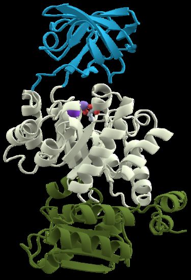
A visual example of the protein domains is shown in Figure 2.2, where is
represented the Pyruvate Kinase, a protein containing three different domains.
3
https://www.ebi.ac.uk/training/online/course/protein-interactions-and-their-importance/
protein-protein-interactions/importance-molecular-i
4
https://www.britannica.com/science/amino-acid
5
https://en.wikipedia.org/wiki/Protein_domain2.2 Biological background 6
Figure 2.2. The protein Pyruvate Kinase, which has three different domains: an all-β
nucleotide binding domain (in blue), an α/β-substrate binding domain (in grey) and an
α/β-regulatory domain (in green)6 .
The knowledge of graphs can be combined with the knowledge of proteins to
create a Protein-protein Interaction Network (PIN), in which the nodes are the
proteins and there is an edge between two proteins A and B (formally (A, B)) when
they are known to physically interact.
Generally, in a PIN, there can be two possible types of edges:
1. Positive edges, between two proteins that are known to physically interact.
2. Negative edges, between two proteins that are known to not interact.
Due to their high importance, the protein-protein interactions are constantly
studied and experimentally detected. One of the most popular and effective methods
for detecting protein-protein interactions is the Yeast two-Hybrid (Y2H) screen.
The Y2H relies on the expression of a specific reporter gene7 . This gene can be
activated by the binding of a transcription factor, composed of two independent
domains: the DNA-binding domain (DB) and the activation domain (AD). These
6
https://en.wikipedia.org/wiki/Protein_domain
7
https://www.singerinstruments.com/application/yeast-2-hybrid/2.2 Biological background 7
Figure 2.3. An overview of the Yeast two-Hybrid assay8 . The bait (in red) is fused to the
DNA-binding domain whereas the prey (in green) is fused to the Activation domain.
If these proteins do not interact, the expression of the reporter gene is not activated
(B), while, if they interact, the reporter gene expression is activated by the activation
domain (C).
domains, since they are functionally and structurally independent, can be fused to
two different proteins. One protein, referred as bait, is fused to the DB domain,
whereas the other, referred as prey, is fused to the AD.
As can be seen from figure 2.3, only when the bait and prey interact the expression
of the reporter gene is possible. Instead, if the two proteins do not interact, the the
activation domain is not able to localize the reporter gene to drive gene expression.
The Y2H experiments can be performed also in a large-scale way, in which a single
bait can be tested, for example, against an array of preys [2], leading to the discovery
of several interaction partners.
8
https://www.singerinstruments.com/application/yeast-2-hybrid/8
Chapter 3
Datasets
One of the problems encountered when retrieving the state-of-the-art systems for
PPI link prediction is that often different datasets were used among different systems,
making a fair comparison impossible.
Indeed, there are a large number of protein-protein interactions databases [24].
The main ones, here referred as primary databases 1 , obtain all of their data by
curating peer-reviewed publications [39, 44, 57, 71]. An example of primary database
is the Biological General Repository for Interaction Datasets (BioGRID), which
currently contains over 380 thousand unique protein-protein interactions only for
the Homo Sapiens organism.
However, in each primary database there are interactions not contained in other
primary databases. Therefore, there are other databases, here referred as secondary
databases, that integrate the contents of multiple primary databases [54, 60]. One of
the most used secondary database is STRING [60], which contains also information
about computationally predicted interactions.
However, with high probability, some of the interactions contained in these
databases (both primary and secondary) are false positives (i.e. they do not exist
although they are reported), making the resulting databases highly biased. This
is also shown in [49], where the authors conducted an experiment to measure the
reliability of the interactions derived from medical literature. Specifically, they
extracted 33,000 literature binary protein interactions and they divided them into
1
Notice that some of them are old or slowly updated [44, 71]9 those reported only in a single publication and detected by only a single method (formally LIT-BS), which accounted for two thirds of the total number of interactions, and those supported by multiple pieces of evidence (formally LIT-BM). Then, they used two protein-protein interaction detection methods, the mammalian protein- protein interaction trap [15] and yeast two-hybrid assay [14], to test the reliability of these two sets (LIT-BS and LIT-BM). As a result, they discovered that the recovery rate for the pairs in LIT-BS was only a bit higher than the one of the random selected protein pairs used as negative control and considerably lower than the recovery rate of the pairs in LIT-BM, showing that only the interactions with multiple pieces of evidence should be considered reliable. At the time the paper was written, the number of these interactions (i.e. those having multiple pieces of evidence) was 11045, which is a very small number with respect to the the estimated size of the human PIN [58]. The proteins in the interactions contained in each database are always associated with an ID that univocally identify them. The most used protein IDs are the UniprotKB IDs, altough other identifiers, such as the Gene names and the Entrez Gene IDs are widely used. Therefore, when two databases using different protein identifiers are used, a mapping from the identifiers used by the first to the identifiers used by the other is required. For example, supposing that one database uses the UniprotKB identifiers while the other uses the Gene names, a specific protein would be identified as P31946 (UniprotKB ID) in the first database while it would be identified as YWHAB (gene name) in the second database. However, the mapping process sometimes could be a source of errors, due to the different structures of the identifiers databases. For example, a specific uniprotKB ID could not be mapped to any (or, more frequently, is mapped to more than one) gene name. During this thesis, several datasets were used: HuRI, LIT-BM, HQND, and some other negative datasets generated by different methods, as will be discussed in Chapter 6. These datasets were used because, although smaller than the majority of primary and secondary databases, they are characterized by a high level of reliability.
3.1 HuRI                                                                                      10

                Proteins          HI-05             HI-14              HI-19
                    HI-05    1570 (100%)        1245 (79%)         1259 (80%)
                    HI-14     1245 (27%)        4523 (100%)        3584 (79%)
                    HI-19     1259 (14%)        3584 (42%)        8490 (100%)
Table 3.1. Overlap among the proteins in the three versions of the HuRI dataset. The
      overlap between the proteins is more consistent with respect to the one of the interactions.
      Indeed, the 79% of the proteins in HI-05 are contained in HI-14, and the same percentage
      is met when comparing the proteins in HI-14 with those in HI-19.

3.1       HuRI

HuRI is the Human Reference Interactome2 . This dataset currently has three
versions:

   1. HI-I-05 [50](HI-05), which contains ~2800 interactions among ~1500 different
        proteins.

   2. HI-II-14 [49](HI-14), which contains ~14000 interactions among ~4500 differ-
        ent proteins.

   3. HI-III-19 [35](HI-19), which contains ~54000 interactions among ~8400 dif-
        ferent proteins.

      Although they are different versions of the same dataset, the overlap between
their interactions and proteins is not so consistent, as shown in Tables 3.1 and 3.2.
      Indeed, regarding the proteins, only 79% of the proteins in HI-05 are in HI-14,
and same percentage is met when comparing the proteins in HI-14 with those in
HI-19. Instead, regarding the interactions, only 27% of the interactions of HI-05 are
also in HI-14, while only 37% of the interactions of HI-14 are contained in HI-19.

      The last version of HuRI (released on April 2019), HI-III-19 (or HI-19), currently
contains about 54496 interactions between 8490 different proteins [35]. All the
interactions in this dataset have been retrieved by a systematic yeast two-hybrid
  2
      http://interactome.baderlab.org/
3.2 LIT-BM 11
Interactions HI-05 HI-14 HI-19
HI-05 2770 (100%) 746 (27%) 773 (28%)
HI-14 746 (5%) 14614 (100%) 5393 (37%)
HI-19 773 (1.4%) 5393 (10%) 54496 (100%)
Table 3.2. Overlap among the interactions in the three versions of the HuRI dataset.
Although they represent different editions of the same dataset, only the 27% of the
interactions in HI-05 are contained in HI-14, whereas only the 37% of the interactions
contained in HI-14 are in HI-19.
screening pipeline and have at least one piece of experimental data. Then, these
interactions were further validated in multiple orthogonal assays, and their quality
turned out to be comparable or greater than the quality of a set of interactions with
more than two pieces of experimental evidence (LIT-BM).
In this dataset, the entries are often protein isoforms (i.e. protein variants
originated from genetic differences), as Q15038-1. However, for some experiments,
we had to convert each protein isoform to the original protein (e.g. Q15038-1 →
Q15038).
The HuRI dataset also contains a wide range of useful information for each
interaction, such as the biological roles of the two proteins in the experiment (e.g.
bait) and the confidence score of each interaction.
The proteins in this database are identified by their UniprotKB IDs and Gene
names.
3.2 LIT-BM
LIT-BM is a database of protein-protein interactions that were retrieved from medical
literature and supported by multiple pieces of evidence, of which at least one comes
from a binary assay type [49]. As previously explained, as a result of the experiment
performed in [49], these interactions are the only ones that should be considered
reliable among all the interactions extracted from medical literature. Indeed, this
dataset has comparable high quality to that of HI-19.3.3 HQND 12
The LIT-BM dataset was downloaded from the Human Reference Protein Inter-
actome website3 and contains 13030 protein interactions among ~6000 proteins. The
main difference between this dataset and the HuRI dataset is that this one, since
the interactions in it are retrieved from the literature, is biased towards well studied
proteins and contains more information in the dense zone of the human Protein
Interaction Network, while the latter, being the result of a screening pipeline, is
more systematic and unbiased.
Among the information for each interaction in LIT-BM, is also present the
mentha-score, that is a confidence score that takes into account all the experimental
evidence retrieved from the different databases4 .
The proteins in this database are identified by their UniprotKB IDs and Gene
names.
3.3 HQND
While the two previous databases (HI-19 and LIT-BM) contain only positive inter-
actions, the High Quality Negative Dataset contains only negative interactions, i.e.
interactions that are known to not exist.
The negative interactions in this dataset are i) not reported in the medical
literature and ii) supported by at least 3 independent orthogonal experimental
methods being negative.
This dataset is not public and has been released to us by the University of
Texas at Austin, in order to perform several experiments. Although it is very
small (676 interactions among ~1200 proteins), its rarity arises from the fact that
the interactions inside it are negative. Indeed, while there are plenty of datasets
containing positive interactions, there are no reliable datasets containing negative
interactions, as will be explained in detail in chapter 5.
The proteins in this database are identified by their Gene IDs.
3
http://interactome.baderlab.org/download
4
http://mentha.uniroma2.it/browser/score.html13
Chapter 4
PPIs prediction review in
literature
Protein-protein interactions (PPIs) are the basis of many biological processes. There-
fore, a thorough understanding of PPIs could lead to a deeper comprehension of the
cell physiology in both normal and disease states, facilitating relevant tasks like drug
target developing and therapy design [1, 3, 10, 70]. Consequently, PPIs prediction,
that is the prediction of new protein-protein interactions given a Protein-protein
Interaction Network, became crucial, both to investigate new associations among
proteins and to check how these associations could contribute to the discovery of
new methods in the biomedical field.
High-throughput technologies1 , like Yeast two-Hybrid screens [14], and literature
analysis have been used to generate a massive amount of data. Two of the most
used high-throughput methods to determine protein-protein interactions are Yeast
two-hybrid (Y2H) screens and Affinity-Purification Mass-Spectrometry (AP-MS).
The main difference between the two is that Y2H is used to identify interactions
between pair of proteins (binary interactions) while AP-MS identifies members of
stable complexes, whether they directly interact with the bait protein or not 2 . Despite
the wide use and the effectiveness of the two aforementioned methods, they are
very expensive and time consuming, revealing the need of high-throughput
1
https://en.wikipedia.org/wiki/Protein%E2%80%93protein_interaction_screening
2
https://web.science.uu.nl/developmentalbiology/boxem/interaction_mapping.html4.1 Connection-based methods 14
computational methods able generate high quality PPIs predictions.
However, there are several problems that make this task difficult to solve, for
example:
1. Absence of explicit encoding of negative knowledge. This problem
arises from the fact that generally only the positive interactions are reported
in the medical literature and consequently contained in the protein-protein
interactions databases. However, also negative interactions are equally useful
when it comes to the training/testing of the PPIs prediction systems. Despite
its importance, the lack of "gold standards" regarding the negative knowledge
is often underestimated by the PPIs prediction systems, leading to biased
performances and metrics. This issue will be discussed in more details in
chapters 5 and 6.
2. Human PIN high incompleteness. This is a problem associated with the
small number of known protein-protein interactions in the human PIN [58, 64].
One of the consequences of this problem is that all the methods that try to
predict new PPIs are strongly limited by the lack of training data.
In fact, according to [34]: Although computational efforts can mitigate the
shortfall of literature-curated efforts and involve minimal experimental cost,
any computational effort would be restricted by current limited knowledge of
biological systems.
Despite the above mentioned problems, the number of systems for PPIs prediction
is huge and constantly growing. These methods can be broadly divided in two
categories: connection-based methods and protein-based methods.
4.1 Connection-based methods
These are the methods that leverage the structural information of the graph.
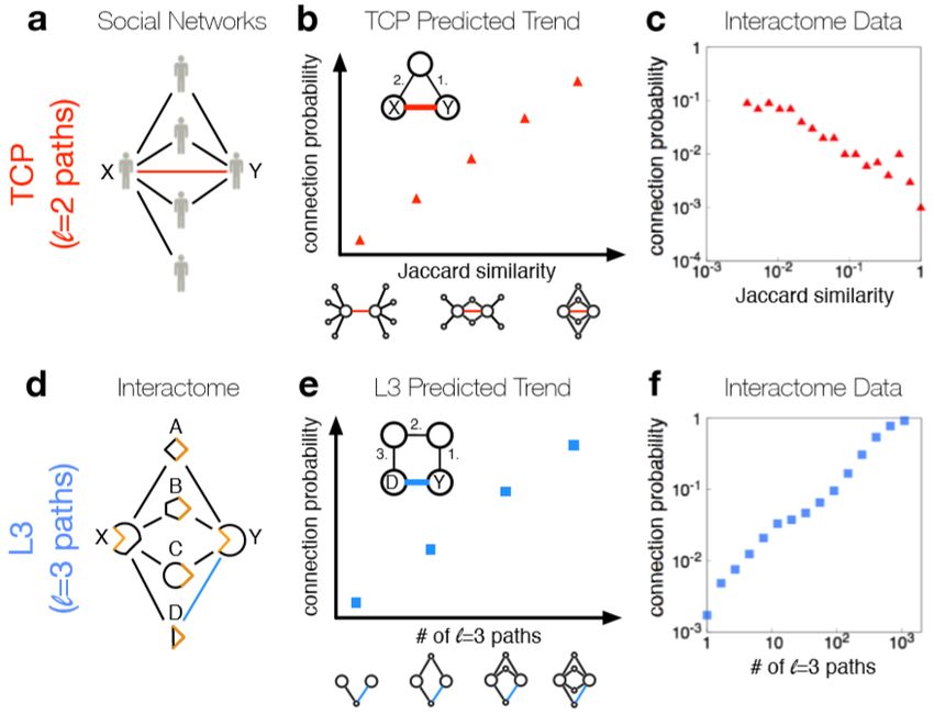
For example, the authors of [26] have shown that the Triadic Closure Principle
(TCP, i.e. that two proteins likely interact if they share multiple interaction partners)
is not valid for most protein pairs. Indeed, from a biological point of view, the4.1 Connection-based methods 15
Figure 4.1. The comparison between the TCP and the L3 principle. Although the TCP
is very effective in social networks (a), it is not as successful in the protein interaction
networks, since the connection probability does not increase with the Jaccard similarity,
as might be expected (b, c). Instead, the L3 principle is effective in the protein interaction
networks, since the connection probability increases with the number of L3 paths (d, e,
f) [26].
interaction of two proteins y and z with an high number of proteins x1 , x2 , .., xn
means that y and z probably have higher interaction profile similarities. Therefore,
since their interaction interfaces are similar, as opposed to complementary, they
will tend not to interact [26, 35]. Instead of TCP, they proposed a link prediction
principle based on paths of length three (L3 principle, figure 4.1). Specifically, they
expect the interaction probability between two proteins A and B to be positively
correlated with the number of paths of length three linking A to B, normalizing this
number to avoid that hubs, since they introduce shortcuts in the network, could
bias the result.
Another example of a connection-based method for PPI prediction is the one
presented in [32]. The idea behind this method is that two nodes having similar
’distances’ to all other nodes in the network can potentially interact with each other.4.2 Protein-based methods 16 To correctly compute the distances, they presented a novel random walk algorithm based on two ideas: (i) a small amount of resistance is added to each edge of the network to encourage the random walker to stay close to the starting point, and (ii) additional resistance is added to discourage the random walk from visiting a new node. The latter condition is introduced to avoid reaching, especially from hubs, nodes that may not be functionally related to the starting node. The result of this procedure is a |V | × |V | probability matrix, where |V | is the number of nodes. Finally, the Pearson correlation between two rows or columns is computed and the pairs of nodes having the correlation above the threshold are considered to be interacting. However, the connection-based methods are strongly limited by data incom- pleteness, since, as explained above, only a small percentage of the total number of protein-protein interactions is known. Furthermore, since these methods explore only network-related information, they are generally not able to properly predict interactions between proteins without known links. For example, applying the link prediction principle discussed in [26] (L3 principle), is not possible to predict an interaction between pairs of proteins not connected by any path of length three. Hence, the connections-based methods should be integrated with other methods using the proteins information (such as the amino acids sequence) to overcome the issue of predicting interactions between proteins not related by any topological property. 4.2 Protein-based methods This category consists of all the methods that leverage the proteins information in order to predict new protein-protein interactions. Specifically, the majority of these methods rely on the proteins’ sequences information in order to predict a score for the probability of their interaction [18, 33, 59, 67, 73]. Indeed, the amino acids sequence of a specific protein can contain relevant information about the protein’s structure and is therefore fundamental to identify possible interactions. Generally, the protein-based methods first construct enriched representations of
4.2 Protein-based methods                                                             17

Figure 4.2. The typical flow of a PPIs prediction system. First, the two proteins of an
   interaction are represented in a more complex way, trying to capture their primary
   characteristics. Then, these representations are given as input to a PPIs prediction
   model (i.e., usually, a machine learning model) which outputs the probability of their
   interaction.

the proteins. For example, the authors of [33], inspired by the "word2vec" model in
Natural Language Processing, created an embedding for each amino acid, considering
proteins’ sequences as documents and amino acids as words. Then, they constructed
an enriched representation of a protein by concatenating the embeddings of the
amino acids in its sequence.
   After their construction, these more detailed representations of the proteins are
given as input to specific models (e.g. deep neural networks) to determine whether
the two input proteins could interact or not.
4.2 Protein-based methods                                                          18

   For example, the authors of [59] used a stacked autoencoder, giving as input
proteins coded into two different ways: Autocovariance method (AC) and Conjoint
Triad method (CT). The AC method [69] is a way to transform a sequence of amino
acids into a N × 7 matrix, where 7 is the number of physicochemical properties
of amino acids that can reflect the various modes of a protein-protein interaction
(hydrophilicity, volumes of sidechainsofaminoacids, polarity, polarizability, solvent-
accessible surface area, hydrophobicity, net charge index of side chains), and N is
the lag used by the formula, which is usually set as 30. Instead, in the Conjoint
Triad method [55], the 20 amino acids are firstly clustered into seven groups, based
on their side chain volumes and their dipole. Then, after replacing each amino acid
with the number of its cluster, a window composed of three amino acids is used to
slide across the sequence, capturing the information about the frequency of each
possible combination of three numbers (from 111 to 777).
   Other examples of deep learning models used for PPIs prediction are those in
[33] and [18], that are, respectively, a CNN followed by a LSTM and a CNN followed
by a random projection module, that helps the model to investigate the combination
of the patterns learned from two inputs proteins and enables the model to ignore
the order of the input profiles. An example of the functioning of a typical PPIs
prediction system is given in Figure 4.2.
   Although the majority of these methods claim to achieve very high accuracies
both on the training sets and on the validation sets, they should be tested under
different datasets and conditions to better understand their predictive power. For
example, the authors of [33] obtained excellent results (accuracy from 92% to 98%)
on six different positive validation sets. However, since they used sets containing
only positive examples, their performances could be incorrect since their model
could be inclined to predict a new interaction as positive (a model predicting always
"positive" would have a perfect accuracy). This hypothesis was also confirmed when
we replicated their model (obtaining comparable results on the external datasets),
and tested in on a dataset containing only negative examples [7], obtaining very
poor results (about 30% accuracy). One of the main reasons for this performance
drop could be related to the bias induced by the choice of negative examples in the
4.2 Protein-based methods   19

training phase.
20

Chapter 5

The negative interactions issue

As mentioned in the previous chapters, the positive interactions are generally reported
in the medical literature and therefore contained in all the databases of protein-
protein interactions. Yet, it is known that the number of positive interactions in the
human PIN is orders of magnitude lower than the number of negative interactions,
since the PIN has a very low density (probably less than 0.005) [58, 64].
   Still, the knowledge about negative protein-protein interactions (hereafter, NPIs)
is very limited, since they are generally considered less valuable than the positive
ones. Despite this, high-quality NPIs are very important for several reasons:

   1. As previously mentioned, machine learning (and, recently, especially deep
      learning) has been widely used to build models designed to discover new PPIs.
      However, these models need to be trained and tested also on high-quality
      negative interactions, to prevent bias and to ensure that the performances and
      metrics reported are not distorted by the choice of inappropriate training and
      testing negative instances.

      For example, analyzing several deep learning models, it seems like, since specific
      negative interactions are used for training, they only learn to distinguish
      the types of negative interactions in the training from the types of positive
      interactions in the training. Consequently, they will have very high accuracy
      on the training and test sets (since these datasets will only contain those
      types of negative and positive interactions), while they will obtain very poor
5.1 Random sampling 21
results when tested on datasets containing positive and negative interactions
of different types. This hypothesis is also confirmed in section 7.3, where some
of these models will be analyzed in more detail.
2. The availability of negative knowledge, when very reliable, could help in decid-
ing which interactions should not be tested in clinical experiments, speeding up
the process of determining new protein-protein interactions. For example, an
experimentally validated NPI between two proteins, could be useful to avoid
testing this interaction again in the future.
3. They could also be useful for the training of specific text mining models
[22]. For example, they are required when distant supervision, which is a
technique adopted to automatically label some training instances, based on
some independent data sources, is used [37].
Despite their importance, currently there are no reliable datasets of negative
interactions, causing a lack of negative "gold standards". Hence, for the training
and testing of the models, NPIs are usually chosen using two different approaches:
random sampling and different subcellular location.
5.1 Random sampling
In this approach, the negative instances are chosen by randomly pairing proteins
and then removing the pairs already included in the positive examples.
Although this approach is currently considered as the most reliable for generating
negative instances and it is widely used by the PPIs prediction systems, it presents
several disadvantages.
One disadvantage of this method is that, since the human PIN is highly incomplete
and we do not know about the majority of the positive interactions, we could choose,
as negative examples, interactions that could exist in reality, and this will add noise
to the training set. However, it should be noted that, because of the low density of
the human PIN, the probability that a negative interaction chosen by the random
sampling approach is, in reality, a positive interaction, is very low (probably <
0.5%).5.1 Random sampling 22
Another disadvantage is that the NPIs generated by this approach are highly
influenced by the presence of hubs in the set of positive PPIs. Indeed, since
they are chosen randomly from the set of non-positive interactions, the probability
that a NPI contains a hub belonging to the set of positive interactions is much lower
than the probability that it contains a protein having a low degree in the positive
set (since, for the way random sampling works, we will be more likely to choose an
interaction between proteins having low centrality degrees). The influence of hubs
is also reported by Yu et al. [72], who showed how the evaluation performances of
different systems drop when it is used, as test set, a negative subset generated by
balanced random sampling, i.e. a negative set where each protein appears as many
times as it does in the positive set.
However, later, Park et al. [40] demonstrated that the NPIs dataset generated
using balanced random sampling is not suitable for testing purposes, since it differs
from the population-level negative subset (i.e. the real negative subset) more than a
negative dataset generated by simple random sampling. On the other hand, in line
with Yu et al. [72], they confirmed how, when the negative instances generated from
random sampling are used to train a model that uses the sequence of the protein as
a feature, the bias induced by the presence of hubs in the positive set contribute,
in an inappropriate way, to increase the performances. Therefore, balanced
random sampling, since it maintains the degree of each proteins and therefore is not
influenced by the presence of hubs, might still be appropriate for training purposes.
Consequently, they suggested two different types of negative subset sampling:
1. The subset sampling used for cross-validated testing, where one prefers unbiased
subsets so that the estimate of predictive performance can be safely assumed to
generalize to the population level. For this type of task, the random sampling
is more suitable than the balanced random sampling, since it is less biased and
closer to reality.
2. The subset sampling used for training, where one desires the subsets that best
train predictive algorithms, even if these subsets are biased. For this type of
task, the balanced random sampling is more suitable than the simple random5.2 Subcellular location heuristic 23
sampling, since its characteristics allow him to avoid the issue regarding the
presence of hubs.
Moreover, the negative protein-protein interactions generated by random sam-
pling are not appropriate for specific biological contexts, where the interaction
probability between proteins is higher than average, as shown in [63].
5.2 Subcellular location heuristic
In this approach, the negative instances are chosen by randomly pairing proteins in
different subcellular locations. Hence, in the negative set generated by this approach
there could not be interactions between two proteins in the Nucleus or two proteins
in the Cytoplasm.
However, although the subcellular location constraint obviously reduces the
number of false negatives, the authors of [5] have shown how this method is highly
affected by bias. Specifically, they showed how the accuracy of a classifier depends
on the co-localization threshold (i.e. the allowed similarity between the cellular
compartments) of pairs of proteins in the negative examples. Indeed, the accuracy
is higher for low co-localization threshold (i.e. using, as negative examples, pairs
of proteins with a strong difference in their subcellular localization), and this can
be explained by the fact that the constraint on localization restricts the negative
examples to a subspace of sequence space, making the learning problem easier than
when there is no constraint.
Furthermore, confirming the previous statement, Zhang et al. [73] trained
the same model using, as negative examples, first, pairs of proteins in different
subcellular locations and next, pairs of proteins retrieved with different methods
(like sequence similarity and length of the shortest paths, as will be explained later).
As a result, the former model (i.e. the one trained using negative interactions derived
from different subcellular locations) performed better on datasets composed only
of positive interactions (96% vs 86%) but much worse on datasets composed only
of negative interactions (4% vs 17%), showing that, when the negative interactions
generated from the different subcellular location strategy are used for training, the5.3 Other methods 24
model is inclined to predict a new protein pair as a positive interaction.
Albeit it has been shown that this approach is highly biased, it is still used in
several recent works [33, 59, 67].
5.3 Other methods
Motivated by the limitations of the existing solutions, a research area has been
focused on how to produce reliable negative examples. The following subsections
contain an analysis regarding the methods proposed.
5.3.1 Bait-prey approach
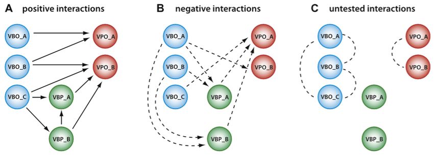
Trabuco et al. [63] proposed a method that generates reliable negative examples
using viability analysis1 . To do this, they retrieved the proteins in the interactions of
the IntAct dataset that were derived from large-scale Y2H experiments, and divided
them into 2 categories: viable baits (VB, i.e. proteins acting as baits for at least one
interaction) and viable prey (VP, similarly defined). Then, a protein is considered
a viable bait only (VBO) if it is a VB but not a VP. Viable prey only (VPO) are
similarly defined. Each link from a VB to a VP that is not present in the dataset of
positive interactions is considered as a negative interaction, since it is assumed to
have been tested (for the way the large-scale Yeast two-hybrid works). Instead, each
link between two VBO or between two VPO is deemed untested, since the proteins
should not have been tested in any way. This method is presented in Figure 5.1.
In order to generate more reliable datasets, the authors also proposed a variant
of their model using a shortest path heuristic, based on the fact that due to the
small-world property exhibited by biological networks [3], interacting proteins are
expected to be near each other in the network. In this variant they removed from the
negative set generated a negative interaction between two proteins A and B if the
shortest path from A to B in the PIN was less than a certain threshold.
Altough the bait-prey method has shown improvements over the random sampling
on the protein-protein interactions networks of different species and organisms (e.g.
1
http://www.russelllab.org/negatives/5.3 Other methods 25
Figure 5.1. The functioning of the viability analysis [63]. (A) the positive interactions
retrieved by the large-scale yeast two-hybrid screens. (B) The negative interactions
generated are those from proteins acting as baits to proteins acting as preys. (C) each
link between two proteins acting only as baits (two VBO) or between two proteins
acting only as preys is not considered as negative interaction, since it is considered to be
untested.
yeast), especially when the shortest path variant was used, it did not show clear
benefits when applied to the human PIN, where the negative interactions generated
using this approach were similar (in terms of performances) to those generated by
random sampling.
This could be partly caused by the human PIN incompleteness issue.
5.3.2 Negatome 2.0
One of the few negative datasets that have been generated is the Negatome 2.0 [7],
which is a database of proteins and protein domains that are unlikely to engage in
physical interactions2 .
The negative interactions contained in this database are retrieved using 2 methods:
(i) analysing, through text mining techniques, a corpus of medical articles, and (ii)
analysing the three-dimensional structures of the proteins.
A first step that is mandatory when trying to retrieve candidate interactions
from the medical literature is that of finding all the sentences that might contain an
interaction, to remarkably decrease the execution time of the method. To address
this problem, the developers used a specific tool, Excerbt [4], to retrieve only the
2
http://mips.helmholtz-muenchen.de/proj/ppi/negatome/5.3 Other methods 26
sentences where: (i) the proteins are both the agent (the entity that carries out the
action of the verb) and the theme (the entity that receives the action of the verb),
(ii) there is a verb referring to interactions or binding and (iii) there is a negation.
Furthermore, the authors defined a confidence score based on simple features, like
the length of the sentence and the type of the relation (some relations are considered
to be stronger than others), to assess the precision of the linguistic analysis. Then,
the precision and the recall of the resulted "non-interactions" have been evaluated
through manual validation.
Regarding the precision, the authors analyzed a sample of the non-interactions
generated, finding that more than 50% of them classified correctly. In addition, it
also turns out that the confidence score was very informative about the annotation
quality. Indeed, among the 20 top scoring sentences the precision of text mining
was 95%, while for the median 20 and the bottom 20 sentences it was 45% and 15%,
respectively. Despite the importance of the confidence score, it is not released by the
authors of the dataset, and it is considered to be internal to the procedure.
To compute the recall, i.e. how many of the non-interactions described in the
literature were found by Excerbt3 , they investigated how well Negatome 1.0 (a small
database derived by the manual curation of the literature) could be reproduced
by text mining. Regarding this measure, the results are unsatisfactory. Indeed,
when they analyzed a sample of 20 non-interactions from Negatome 1.0, they found
out that only five non-interactions were "reachable" from Excerbt, and only 3 of
them were correctly identified. Among the others 15 non-interactions, one was
misclassified by Negatome 1.0, and the remaining 14 could not be found by Excerbt,
since they were present in sentences containing particolar grammar features (e.g.
ellipsis, anaphora) or protein names not covered by the Excerbt ontology.
Overall, the system exhibits a very low recall and a not good enough precision.
Moreover, considering the number of positive interactions already known and the
fact that negative interactions should be considerably more than the positives, the
number of non-interactions contained in Negatome is very small, less than 2000.
3
http://mips.helmholtz-muenchen.de/excerbt/5.3 Other methods 27
5.3.3 Sequence similarity and shortest paths
Very recently, Zhang et al. presented two novel methods for generating negative
protein-protein interactions [73].
The first one selects pairs of proteins having a lower sequence similarity score,
based on the idea that for an experimentally validated PPI between protein i and
j, if a protein k is dissimilar to i, there is a low possibility that k interacts with j.
To do this, they first calculated the sequence similarity score using the BLOSUM50
matrix, and then they normalized the score using the following formula:
bl (i, j) − min {bl (i, 1) , ..., bl (i, n)}
bl
e (i, j) = (5.1)
max {bl (i, 1) , ..., bl (i, n)}
Where n represents the number of proteins and bl (i, j) is the score of the
BLOSUM50 matrix for proteins i and j.
However, Luck et al. [35] have shown that, even if global sequence identity is
indicative of shared interaction interfaces, it likely fails to identify pairs of proteins
whose shared interaction interface is small and that the functional relationships
between proteins are not necessarily identified by sequence identity.
Instead, the second method selects negative interactions based on the following
observation: the probability, for a pair of proteins, to share similar functions (so
to interact) reduces with the increase of the length of the (shortest) path between
the two proteins. However, as also mentioned in section 3.1, the authors of [26]
have shown that the principle that two proteins are likely to interact if they share
multiple interaction partners, that can also be called L2, is not valid for PPI networks.
Furthermore, they have shown that the connection probability varies using different
path lengths, demonstrating that there is no clear correlation. Hence, the assumption
on which the second method of negative interactions generation is based (i.e. that
two proteins are more likely to interact if the path between them is shorter), could
be partly unfounded.5.3 Other methods 28 5.3.4 Hybrid methods Finally, there are some methods that use cellular compartment information (CCI) and other information to generate high-quality NPIs, stating that the two proteins in each pair should not have overlap in any of these areas (i.e. they should have different cellular compartment, different functions, etc.) [51, 56]. Yet, if only the use of different CCI led to biased results since the constraint makes the task easier and the performance biased, as shown in [5], imposing a filter using the intersection between CCI and other constraints, even though it obviously reduces false positives even more, could worsen the problem.
29

Chapter 6

Comparison of methods
generating negative interactions

We performed several experiments in order to assess the reliability of the negative
interactions generated by two of the previously explained methods: random sampling
(section 5.1) and bait-prey (subsection 5.3.1, [63]). The former was chosen because it
is widely used and surely less biased than the different subcellular location approach,
and the latter was chosen because, although not extensively used, its premises classify
it as one of the most reliable methods among those described in chapter 5.
       Both of these methods, to generate negative interactions, need a training set
of positive interactions, from which the set of proteins will be extracted. For this
purpose, we decided to consider the 5393 interactions contained both in HI-14 and
HI-19 as high-quality positive interactions, and, from now on, they will be referred
as HI-19-TRAIN.
       First, we considered the set P of proteins in HI-19-TRAIN (2642 different
proteins)1 .
       Using the set of 5393 positive interactions in HI-19-TRAIN (i.e. the interactions
between pairs in P which are in HI-14 and are also present in HI-19), different
sets of negative interactions, GN I(P ), were generated, using the random sampling
   1
       It should be noted that the proteins in HI-19-TRAIN are only a subset of the proteins in
the intersection between HI-14 and HI-19. Indeed, a protein present in both datasets that is not
contained in a common interaction is not present in HI-19-TRAIN.
30
approach, the bait-prey, and some variations of the latter.
One of the available ways to test the quality of the negative interactions generated
by these methods is to calculate the number false negative interactions (i.e. predicted
negative interactions that were instead positive).
Since these methods, for how they work, can only generate negative interactions
between proteins in P, the positive interactions that can be used as "ground truth"
are only those between the same set of proteins P, that are in HI-19 (that
also represents our test set) and are not in HI-14 (since, if they are both in HI-19
and in HI-14, they would be contained in the training set HI-19-TRAIN). These
positive interactions, that represent our test set, will be, from now on, referred as
HI-19-TEST, and their number is 10358 (|HI-19-TEST|= 10358).
For clarification, figure 6.1 presents a graphical view of all the possible interactions
between a set of proteins P.
In this figure:
1. N I(P ) are all the existing negative interactions among pairs of proteins in P.
2. P I(P ) are all the existing positive interactions among pairs of proteins in P.
3. KP I(P ) are the known (tested) positive interactions between proteins in P. In
our case, KP I(P ) is represented by the interactions in HI-19 between proteins
in P. Each of these interactions will be in HI-19-TRAIN if it is contained also
in HI-14 and will be in HI-19-TEST otherwise.
4. KN I(P ) are the known (tested) negative interactions between the proteins in
P. In our case, KN I(P ) is represented by the interactions in HQND between
proteins in P.
5. GN I(P ) are the generated negative interactions between proteins in P . The
negative interactions generated by a specific method m (see Chapter 5) will
be referred as GN Im (P ).
On the basis of these sets, several evaluation metrics were defined: Verified Error
Rate, Minimum bound of Error Rate, Verified Success Rate and Approximated True
Error Rate.6.1 VER and MER 31
Figure 6.1. Diagram of positive and negative interactions between a set of proteins P .
N I(P ) are the negative interactions between proteins in P, whereas P I(P ) are the
positive ones. KN I(P ) are the known negative interactions between proteins in P,
which, in our case, are a subset of all the negative interactions in HQND. Instead,
KP I(P ) are the known positive interactions between proteins in P, that are, in our
case, a subset of the interactions contained in HI-19. Each method m generates a
set of negative interactions, in the figure denoted as GN I(P ). Finally, A and B are,
respectively, the negative interaction generated which are known to be positive and
those which are known to be negative. Please note that the proportions of the sets in
the figure do not reflect reality.
6.1 VER and MER
Considering the sets in figure 6.1, the Verified Error Rate (VER) of a specific method
m can be defined as:
GN Im (P ) ∩ KP I (P )
V ER = (6.1)
KP I (P )
That is the fraction of known positive interactions (KP I(P )) that were generated
as negative interactions by the method m (GN Im (P )). This measure quantifies how
good the method is at avoiding the generation of positive interactions with respect
to the number of positive interactions known.
Obviously, this measure is strictly related to the number of interactions generated6.1 VER and MER 32
by the method, since, for example, a simple method not generating any negative
instance would have a perfect score (0% VER).
Instead, the Min. bound of Error Rate (MER) of a specific method m can be
defined as:
GN Im (P ) ∩ KP I (P )
M ER = (6.2)
GN I (P )
That is the fraction of the negative interactions generated that were instead
positive (false negatives). This measure defines a lower bound on the real error rate
of the negative interactions generated.
We generated negative interactions with four different methods, and the overall
results are presented in Table 6.1.
As first method, the bait-prey approach [63] was used to obtain about 2.32
million negative interactions. The interactions that turned out to be incorrect (based
on the "ground truth" of the 10358 interactions in HI-19-TEST) were 8618 (83%
VER). In relation to the total number of negative interactions generated, the wrong
ones represent the 0.37% (MER).
In the same way, we generated 2.32 million negative interactions using the
random sampling approach2 . The interactions that turned out to be incorrect
were 6856 (66.2% VER). In relation to the total number of generated negative
interactions, we also obtained better results with respect to the bait-prey approach,
since the wrong interactions represent the 0.294% (MER) of the total number of
negative interactions generated. For the negative interactions generated by the
random sampling approach, since they are randomly chosen, the experiment has
been repeated 50 times, taking the average of the wrong interactions at the end.
Given how random sampling works, the number of generated interactions does not
affect the MER (i.e. it can generate a different number of interactions maintaining a
2
Note that, differently from the bait-prey approach, the number of negative interactions generated
by the random sampling approach must be set.6.1 VER and MER 33
Generated Wrong Verified Error Minimum Error
Method
NI Interactions Rate (VER) Rate (MER)
Bait-prey 2.32 million 8618 83% 0.37%
2.32 million 6856 ± 55 66.2% ± 0.5 0.294% ± 0.002
Random sampling 785 thousand 2318 ± 17 22.38% ± 0.16 0.295% ± 0.002
705 thousand 2077 ± 15 20.05% ± 0.14 0.294% ± 0.002
Modified
785 thousand 2625 25.3% 0.33%
Bait-prey
Modified &
Filtered 705 thousand 1067 10.3% 0.15%
Bait-prey
Table 6.1. Comparison of the error rates on the HI-19 test set. The best results are
obtained by the MFB-P method, which generates a set of interactions in which only the
0.15% are wrong.
similar MER). However, the VER, as described previously, is highly dependent on
the number of interactions generated. Therefore, the experiment with the random
sampling approach was repeated several times with different sizes, considering the
number of interactions generated by the three other methods, as reported in table
6.1.
Then, trying to improve the bait-prey approach, we considered only the interac-
tions from Viable Bait Only to Viable Prey Only (i.e. a subset of the interactions
generated by the original bait-prey method). This modification, from now on referred
as Modified Bait-Prey (MB-P) method, generated 785 thousand negative interactions,
of which 2625 were wrong (25.3% VER). In relation to the total number of negative
interactions generated, the wrong ones represent the 0.33% (MER). Hence, the
change proposed led to an increase in the quality of the interactions generated with
respect to the original bait-prey approach. Nonetheless, MER and VER are still
higher than those of the random sampling approach (0.33% vs 0.294% and 25.3%
vs 22.38%) and this difference turned out, after a one-tail test, to be statistically
significant (p < .00001).You can also read