Multilateration with Self-Calibration: Uncertainty Assessment, Experimental Measurements and Monte-Carlo Simulations
←
→
Page content transcription
If your browser does not render page correctly, please read the page content below
Article
Multilateration with Self-Calibration: Uncertainty Assessment,
Experimental Measurements and Monte-Carlo Simulations
Joffray Guillory * , Daniel Truong and Jean-Pierre Wallerand
Laboratoire Commun de Métrologie LNE-Cnam (LCM), Conservatoire National des Arts et Métiers (Cnam),
1 Rue Gaston Boissier, 75015 Paris, France; daniel.truong@cnam.fr (D.T.); jean-pierre.wallerand@cnam.fr (J.-P.W.)
* Correspondence: joffray.guillory@cnam.fr
Abstract: Large-volume metrology is essential to many high-value industries and contributes to the
factories of the future. In this context, we have developed a tri-dimensional coordinate measurement
system based on a multilateration technique with self-calibration. In practice, an absolute distance
meter, traceable to the SI metre, is shared between four measurement heads by fibre-optic links. From
these stations, multiple distance measurements of several target positions are then performed to, at
the end, determine the coordinates of these targets. The uncertainty on these distance measurements
has been determined with a consistent metrological approach and it is better than 5 µm. However,
the propagation of this uncertainty into the measured positions is not a trivial task. In this paper, an
analytical solution for the uncertainty assessment of the positions of both targets and heads under a
multilateration scenario with self-calibration is provided. The proposed solution is then compared to
Monte-Carlo simulations and to experimental measurements: it follows that all three approaches are
well agreed, which suggests that the proposed analytical model is accurate. The confidence ellipsoids
provided by the analytical solution described well the geometry of the errors.
Citation: Guillory, J.; Truong, D.;
Keywords: large-volume metrology; multilateration with self-calibration; uncertainty assessment
Wallerand, J.-P. Multilateration with
Self-Calibration: Uncertainty
Assessment, Experimental
Measurements and Monte-Carlo
Simulations. Metrology 2022, 2,
1. Introduction
241–262. https://doi.org/10.3390/ We have developed a three-dimensional coordinate measurement system based on
metrology2020015 an absolute distance meter [1–3]. With the use of four stations, called measurement heads,
Academic Editors: Stephen Kyle,
distributed through a large volume and a multilateration technique, the positions of targets
Stuart Robson and Ben Hughes
can be determined at a micrometric scale. With the use of self-calibration, the knowledge
of the positions of the heads is not even necessary, only distance observations of at least
Received: 24 March 2022 6 targets [4] from our four measurement heads are required.
Accepted: 5 May 2022 In this system, each distance is determined by measuring the phase accumulated by a
Published: 11 May 2022 Radio Frequency (RF) modulated light during its propagation in air up to a target. Indoors,
Publisher’s Note: MDPI stays neutral in a controlled environment, and if the received power is sufficient, the accuracy for a
with regard to jurisdictional claims in displacement measurement is around 2 µm (k = 1) up to 100 m. For absolute distance
published maps and institutional affil- measurements, the accuracy is limited by the mechanical design of the measurement heads
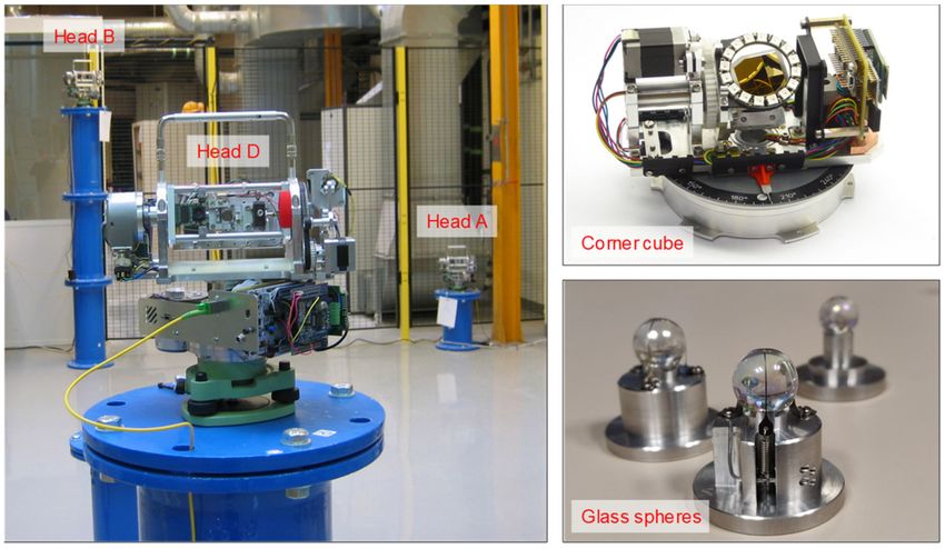
iations. and of the targets depicted in Figure 1. The measurement heads, which play the role of
aiming system, consist of a gimbal mechanism for rotation of the laser beam in every
direction of space, and around an invariant point in space, to hit any targets. The target is a
retroreflector, either a corner cube that can be oriented in any direction, or a sphere of glass
Copyright: © 2022 by the authors. refractive index n = 2. The model of the global error on an absolute distance measurement
Licensee MDPI, Basel, Switzerland.
has been studied in [2,3]: it has been demonstrated that the error due to the developed
This article is an open access article
system follows a distribution close to a Gaussian one with a mean of zero and a standard
distributed under the terms and
deviation σsystem around 5 µm.
conditions of the Creative Commons
Attribution (CC BY) license (https://
creativecommons.org/licenses/by/
4.0/).
Metrology 2022, 2, 241–262. https://doi.org/10.3390/metrology2020015 https://www.mdpi.com/journal/metrology
Metrology 2022, 2                                                                                                    242

                    Figure 1. Three of the four measurement heads (identified by letters) and the two types of targets.

                          The measured distances must also be corrected by the air refractive index. In practice,
                    this index is determined using an updated Edlén equation [5] and data from environmental
                    sensors.
                          Let di,j ◦ be the true distances between the m measurement heads (of index i with m = 4
                    in our experiments) and the n targets (of index j with n ≥ 6), and ni,j be the random noise
                    affecting these distances. Thus, the measured distances are equal to:

                                                             di,j = di,j ◦ + ni,j                                    (1)

                          Our objective is to assess with a consistent metrological approach the uncertainties
                    of the target positions obtained with such a coordinate measurement system. The study
                    of this paper is applicable to any multilateration system such as those presented in [6,7]
                    and based on laser tracking interferometers, the one presented in [8] and based on laser
                    tracking absolute distance meters (repeatability of about 3.4 µm) or the one presented
                    in [9] and based on absolute distance meters using the Frequency Scanning Interferometry
                    technique (uncertainty of 5 ppm including air refractive index). In these works, the results
                    from the multilateration technique with self-calibration have been compared to reference
                    positions provided by a coordinate measuring machine, a calibrated Zerodur® hole plate
                    standard, or a commercial laser tracker. For target without movements, the observed
                    deviations between the measured positions and the reference ones were below 5 µm in [6]
                    for a measurement volume of less than 1 m3 , and submicrometric in [7] for a measurement
                    volume of 5 m × 4 m × 2 m. The deviations, expressed as standard deviation, were equal to
                    about 18 µm for a measurement volume of 1 m3 in [8] and to about 40 µm for a measurement
                    volume of 10 m × 5 m × 2.5 m in [9].
                          The uncertainties of the target positions depend obviously on the uncertainties on the
                    measured distances, but they also depend on the multilateration algorithm, wherein the
                    geometric arrangement of the heads relatively to the targets plays a determinant role. First,
                    if a large number of measurements are made, the repeatability and reproducibility over
                    positions can be quantified (uncertainty called “type A” and characterized by experimental
                    standard deviations), and if different configurations are tested, the contribution of the
                    different input parameters can be identified [10,11]. Such an approach is difficult to imple-
                    ment in our case, simply because a single multilateration measurement requires several
                    hours. Then, the input uncertainties can be propagated to assess the output uncertainties,
                    which is a statistical method frequently applied. However, in some cases, the identifica-
                    tion of models to propagate the uncertainties appears to be particularly difficult, like in
                    multilateration with self-calibration where the positions are determined by minimizing
                    the sum of square errors. Monte Carlo simulations can then be adopted to cope with the
                    uncertainty propagation problem [12], even if they are computationally intensive and time
                    consuming since they require hundreds or thousands of simulations, especially for complex
Metrology 2022, 2                                                                                                        243

                    models. Other approaches than sampling-based methods could be also considered for un-
                    certainty quantification, like approaches based on metamodels. This consists of formulating
                    a mathematical function (a metamodel, i.e., a surrogate) that describes the relation between
                    the inputs (e.g., measured distances) and the outputs (e.g., positions), then computing
                    the output statistics by using the generated mathematical function. Such approaches are
                    presented in [13,14]. Lastly, the uncertainties can be assessed by extrapolating discrepancies
                    between calculated results (resulting from code) and relevant experimental data [15].
                           This paper provides analytical solutions for uncertainty assessment of every target
                    under any multilateration scenario. Indeed, the different multilateration techniques have
                    been studied, from the classical approach where the positions of the measurement heads are
                    assumed to be known and error free to the more advanced approach with self-calibration,
                    i.e., where the positions of the heads are totally unknown. The different processing elements
                    necessary for the implementation of the multilateration algorithm with self-calibration
                    are thus explained step by step. Moreover, this paper proposes a new way to assess the
                    uncertainties of the target and head positions for self-calibration. In [7,9], some positions are
                    fixed for the origin and the orientation of the multilateration frame and have uncertainties
                    equal to zero. The uncertainties of the other positions are derived from the non-linear
                    least-squares solver used for multilateration with self-calibration. In the mathematical
                    approach we proposed, the uncertainties are distributed among all the positions so as not
                    to obtain zero uncertainties on some positions and excessive uncertainties on others. Thus,
                    the result is independent of the multilateration frame chosen by the user.
                           The work is organized as follows: Section 2 presents the multilateration technique
                    when the positions of the heads are perfectly known, Section 3 when they are affected
                    by position errors, and Section 4 when they are unknown and so when a self-calibration
                    method is adopted. These sections explain how to solve each of these specific problems, and
                    how to assess the uncertainties on the target positions in each of these cases. The original
                    point here is the solution proposed for the multilateration algorithm with self-calibration,
                    the other approaches being already studied in detail in the literature. Nevertheless, all these
                    different cases are treated in this paper because the solution to the self-calibration problem
                    is based on them. Section 5 compares, in the case of the multilateration with self-calibration,
                    the uncertainties calculated analytically to Monte-Carlo simulations and to experimental
                    measurements made with our coordinate measurement prototype designed in house.

                    2. Multilateration with Measurement Head Positions Perfectly Known
                    2.1. Determination of the Target Position
                           The classical multilateration problem consists of determining the coordinates of
                    one target T from a set of several measurement heads Hi located at known coordinates
                    [xHi , yHi , zHi ], and performing distance measurements di up to this target. The true distance
                    between one of these heads and the unknown target position [xT , yT , zT ] is:
                                                               q
                                  di ◦ ( x T , y T , z T ) =       ( x T − x Hi )2 + ( y T − y Hi )2 + ( z T − z Hi )2   (2)

                         From a geometrical point of view, the target position is located at the intersection of
                    spheres centered on the measurement heads and of radius equal to the distances measured
                    by the absolute distance meter. At least four measurement heads are required to obtain
                    a unique solution. Nevertheless, in practice, the use of three heads can be sufficient: this
                    leads to two solutions, but the ambiguity can be resolved with basic assumptions based on
                    the application.
                         In other words, with algebraic terms, when the number of distance measurements is
                    higher than the number of unknown variables to estimate (i.e., the three coordinates of the
                    target), the localization problem can be solved. However, due to uncertainties associated to
                    the distance measurements, the target position should be determined using a non-linear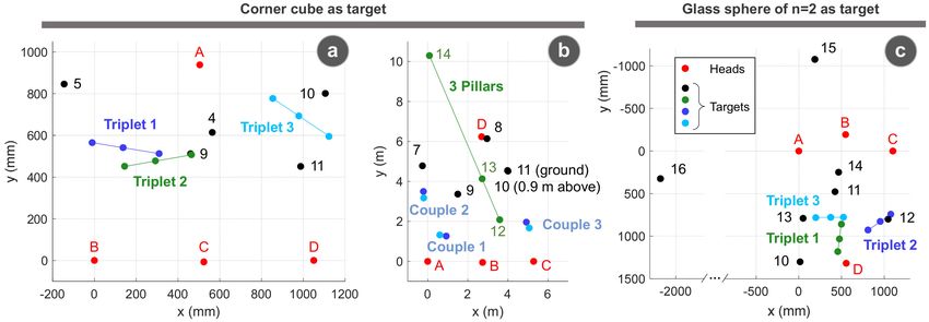
Metrology 2022, 2 244
least-squares approach where the optimal coordinates [xT , yT , zT ] of the target T are those
which minimize the following quantity:
m
cost function = ∑ ( di ( x T , y T , z T ) − k Hi − T k)2 (3)
i =1
where k.k denotes the Euclidian norm of a vector and di (xT , yT , zT ) is the distance measured
between the measurement head Hi and the target T. It is assumed that the measured dis-
tances are affected by an additive random zero-mean Gaussian noise of known covariance.
To solve the multilateration problem of Equation (3), an iterative Gauss–Newton
algorithm has been adopted. Indeed, Equation (3) is non-linear with unknown parameters
vector [xT , yT , zT ]. Linearizing it via a Taylor series expansion is one possible solution.
Thus, an estimate of the coordinates of the target is first assumed, T0 = [xT0 , yT0 , zT0 ]. Then,
from this estimate, the approximation of the measured distances di (xT , yT , zT ) is obtained
using a first-order Taylor expansion:
di ( x T , y T , z T )
∂di ( x T ,y T ,z T ) ∂di ( x T ,y T ,z T ) ∂di ( x T ,y T ,z T )
≈ di ( x T0 , y T0 , z T0 ) + ∆x + ∆y + ∆z
∂x T x T0 ∂y T x T0 ∂z T x T0
y T0 y T0 y T0
z T0 z T0 z T0
x T − x Hi y −y z T −z Hi
≈ di ( x T0 , y T0 , z T0 ) + ∆x + d ( xT ,y Hi,z ) ∆y + ∆z
di ( x T ,y T ,z T ) x T0 i T T T x T0 di ( x T ,y T ,z T ) x T0
y T0 y T0 y T0
z T0 z T0 z T0
x T0 − xi y T0 −yi z T0 −zi
≈ di ( x T0 , y T0 , z T0 ) + di ( x T0 ,y T0 ,z T0 )
∆x + d ( x ,y ,z )
∆y + d ( x ,y ,z
∆z
i T0 T0 T0 i T0 T0 T0 )
(4)
with ∆x = (xT − xT0 ), and similarly for ∆y and ∆z. Arranged in a matrix form, this gives:
∆x
∆d = J × ∆y (5)
∆z
where ∆d is a column vector equal to the differences between the measured distances and
the approximate ones:
∆di = di ( x T , y T , z T ) − di ( x T0 , y T0 , z T0 ) (6)
and where J is a n × 3 matrix whose row numbered i corresponds to the derivatives:
y T0 −y Hi
h i
x T0 − x Hi z T0 −z Hi
Ji = di ( x T0 ,y T0 ,z T0 ) di ( x T0 ,y T0 ,z T0 ) di ( x T0 ,y T0 ,z T0 ) (7)
The error correction vector is then calculated as follows:
∆x
−1
∆y = J T J × J T × ∆d (8)
∆z
From this result, the estimate of the target coordinates T0 is updated. In practice, this
Gauss–Newton recursive process is repeated until the coordinates of the error correction
vector are small enough.
x T0 + ∆x
T0 updated = y T0 + ∆y (9)
z T0 + ∆z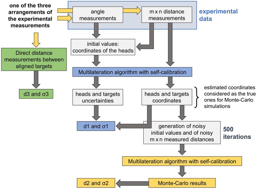
Metrology 2022, 2 245
This method is simple to implement and provide accurate results. Nevertheless, it is
not the only way to resolve a multilateration problem with measurement head positions
perfectly known, other approaches are proposed in the literature [16–19].
Lastly, to take into account the potential different uncertainties on the measured
distances, a weighted least-squares method can be implemented by introducing the weight
matrix W = cov(d)−1 . In such a case, the error correction vector is calculated as follows
(Gauss-Markov theorem [20]):
∆x
−1
∆y = J T W J × J T × W × ∆d (10)
∆z
The covariance matrix of the measured distances, cov(d), is a m × m square matrix
of indices a (rows) and b (columns) which depends on the variances of the distances di
measured by the heads i:
2
di for a = b and i = a
cov(d) = (11)
0 otherwise
2.2. Uncertainty Assessment and Confidence Ellipsoid
To establish how sensitive is the estimate of a target position with respect to the inac-
curacy of the distance measurements, but also with respect to the geometric arrangement
of the system, the Cramér-Rao Lower bound (CRLB) is widely used. This is a well-known
result of the mathematical statistics that gives a lower bound of the covariance of the
estimated target position T [21,22].
cov( T ) ≥ CRLB (12)
In the case of an efficient and unbiased localization algorithm (called estimator in
estimation theory), the lower bound will be reached, which is the case for the localization
algorithm presented in the preceding part and for our experiments where the measured
distances are characterized by a zero-mean Gaussian noise.
In practice, this was determined from a first-order Taylor expansion of the measured
distances. As shown in Formula (8), the residual error on the target position along the
three axes, ∆T = [∆x ∆y ∆z]T , can be expressed as a function of the differences ∆d between
the measured distances and the approximate ones. Thus, using the law of propagation of
uncertainty, it can be written:
−1 −1
cov( T ) = J T J J T cov(d) J J T J (13)
with cov(T) = cov(∆T), and cov(d) defined in Formula (11).
The uncertainty σT on the target position, for a confidence region of one-sigma (i.e.,
68%), can then be deduced as follows:
q
σT = Trace(cov( T )) (14)
where Trace is an operator that returns the sum of the diagonal elements of the matrix.
The covariance of T is a symmetric matrix. Therefore, there are orthonormal vectors v1 ,
v2 and v3 in which cov(T) is a diagonal matrix, called Q. These vectors are the eigenvectors
of cov(T), with corresponding eigenvalues λj . v1 corresponds to the direction with the
highest uncertainty, while v3 corresponds to the direction with the lowest uncertainty.
λ1 2
0 0
Q= 0 λ2 2 0 (15)
0 0 λ3 2
Metrology 2022, 2                                                                                                    246

                         By this way, we define the confidence ellipsoid depicted in Figure 2 whose axes are in
                    the direction of the eigenvectors and the corresponding eigenvalues give half the length of
                    the axes. These parameters are obtained by proceeding to a singular value decomposition
                    (SVD) of cov(T).

                    Figure 2. Confidence ellipsoid.

                          This confidence ellipsoid approximates a confidence region of 20% around a measured
                    target position in space. In general, confidence regions of 68%, 95% and 99% are used. To
                    obtain them, scaling factor of, respectively, 1.88, 2.79 and 3.58 are applied to move towards
                    a trivariate error distribution under the assumption that the uncertainties follow Gaussian
                    distributions [23,24].

                    2.3. Best Arrangements for Multilateration with 4 Heads
                         The optimal arrangement that minimized the uncertainty for a configuration with four
                    measurement heads has been studied in [25]. There are three possible arrangements. First,
                    in Figure 3a, the geometry formed by the four heads can be a regular tetrahedron with the
                    target located at the centre. Then, in Figure 3b, the four heads can be distributed regularly
                    on a circle with an angle between two adjacent head-target vectors equal to 70.53◦ . Lastly,
                    in Figure 3c, the geometry formed by the four heads can be an isosceles tetrahedron with
                    the target located slightly outside.

                    Figure 3. Best arrangements for multilateration with 4 heads: there are three types of geometry (a–c)
                    that minimize the uncertainty on the target position.

                         In these three cases, the uncertainty is equal to its minimum value, i.e., k × σd /
                    sqrt(m) = 1.5 × σd , with k = 3 the number of the dimensional space, m = 4 the number of
                    measurement heads, and σd the uncertainty on the measured distances [26]. This means
                    that our coordinate measurement system, with uncertainties on the measured distances
                    around 5 µm and assuming the positions of the measurement heads known and error free,
                    will not have an uncertainty of less than 7.5 µm.

                    3. Multilateration in the Presence of Uncertainties on the Measurement
                    Head Positions
                    3.1. Determination of the Target Position
                         Up to now, only two influencing factors have been considered: the distance errors and
                    the geometry. In this part, the errors made on the positions of the measurement heads are
                    also considered. To resolve it, we have adopted the localization method presented in [27].
                         The true distances di ◦ and the true coordinates of the measurement heads Hi ◦ are
                    affected by additive random zero-mean Gaussian noises of known covariance. Let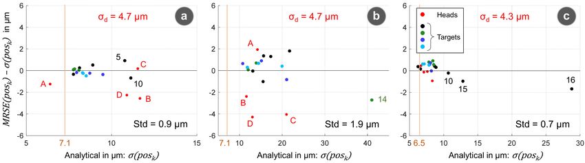
Metrology 2022, 2 247
nd = [nd1 nd2 . . . ndm ]T be the first error vector and nH = [nxH1 nyH1 nzH1 . . . nzHm ]T be
the second one.
d i = d i ◦ + n di
x H = x H ◦ + nx
i i Hi
◦+n (16)
y H i
= y H i y H
z = z ◦+n i
Hi Hi zH i
The unknown true target position T ◦ = [xT ◦ , yT ◦ , zT ◦ ] should so satisfy a system of m
equations described in the following form:
(di − ndi )2 =( x T ◦ − ( x Hi − n xHi ))2 + · · ·
2 (17)
y T ◦ − y Hi − nyHi + (z T ◦ − (z Hi − nzHi ))2
When second order noise terms are ignored, we obtain m equations of the form:
di 2 − 2 di ndi = x T ◦ 2 + y T ◦ 2 + z T ◦ 2 − 2 ( x T ◦ x Hi + y T ◦ y Hi + z T ◦ z Hi ) . . .
+2 x T ◦ n xHi + y T ◦ nyHi + z T ◦ nzHi + x Hi 2 + y Hi 2 + z Hi 2 . . . (18)
−2 x Hi n xHi + y Hi nyHi + z Hi nzHi
Let A be a m × 4 matrix containing the position information of the measurement heads
and B a column vector:
1 −2 x H1 −2 y H1 −2 z H1
1 −2 x H2 −2 y H2 −2 z H2
A= . (19)
.. .. ..
..
. . .
1 −2 x Hm −2 y Hm −2 z Hm
d1 2 − x H1 2 + y H1 2 + z H1 2
d2 2 − x H2 2 + y H2 2 + z H2 2
B= (20)
..
.
dnm 2 − x Hm 2 + y Hm 2 + z Hm 2
Therefore, the system of Equation (18) can be written in this form:
xT ◦ 2 + yT ◦ 2 + zT ◦ 2
xT ◦
B = A× + e1 (21)
yT ◦
zT ◦
with e1 the error matrix:
d1 0 0
0 d2 0
e1 = 2 × nd + 2 × . . .
.. ..
. .
0 0 ... dm
◦ ◦ (22)
x T − x H1 y T − y H1 z T ◦ − z H1
01×3
.. .. ..
nH
. . .
01×3 x T ◦ − x Hm y T ◦ − y Hm z T ◦ − z Hm
= Nd × nd + NH × n H
The system of Equation (21) is non-linear with respect to the coordinates of the target
xT ◦ , yT ◦ and zT ◦ . However, if we assume that xT ◦ 2 + yT ◦ 2 + zT ◦ 2 is independent of the
variables xT ◦ , yT ◦ and zT ◦ , which is mathematically non-rigorous, the system can be
Metrology 2022, 2 248
resolved, but at the cost of inaccurate results. Let T1 be a first approximation of the result
of this system of equations:
xT 2 + yT 2 + zT 2
xT T −1
× AT × B
T1 = = A A (23)
yT
zT
In practice, to take into account the error e1 , a weighted least-squares method is
implemented with the weight matrix W 1 = E[e1 e1 T ]−1 (Gauss-Markov theorem [20]):
xT 2 + yT 2 + zT 2
xT T −1
A T W1 × B
T1 = = A W1 A (24)
yT
zT
with: −1
W1 = Nd Cov(d) Nd T + NH Cov( H ) NH T (25)
The calculation of the weight matrix W 1 , and more precisely NH , requires the knowl-
edge of the true target position T ◦ . However, the latter can be replaced by a first estimate of
the target using Equation (23) or applying the algorithm presented previously in Section 2.1.
For a better estimate, a second step is then performed to determine a second ap-
proximation of the true value T ◦ . Let first ∆T be the error on the approximation made
previously:
xT 2 + yT 2 + zT 2
xT
T1 =
yT
zT
(26)
xT + yT ◦ 2 + zT ◦ 2
◦ 2
∆x T 2 + 2x T ◦ ∆x T + ∆y T 2 + 2y T ◦ ∆y T + ∆ZT 2 + 2z T ◦ ∆z T
xT ◦ ∆x T
= +
yT ◦ ∆y T
zT ◦ ∆z T
A new matrix D is then defined from the square of the coordinates of T1 .
xT 2 + yT 2 + zT 2 T1 (1)
xT 2 T1 (2)2
D= = (27)
yT 2 T1 (3)2
zT 2 T1 (4)2
From the Formula (26), and ignoring the second order noises, D can also be expressed
as follows:
1 1 1 ◦2 1 0 0 0
∆x T
1 0 0 x T ◦
◦2 +
0 2x T 0 0 × ∆y T
0 1 0 × yT
D=
2y T ◦
0 0 0
zT ◦ 2 ∆z T
0 0 1 0 0 0 2z T ◦ (28)
◦ 2
xT
= C × y T ◦ 2 + NT × ∆T
zT ◦ 2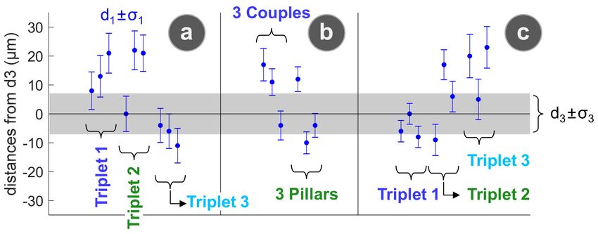
Metrology 2022, 2 249
Thus, the square of the true value of T ◦ can be approximated as:
xT ◦ 2
−1
T2 = y T ◦ 2 = C T C × CT × D (29)
◦ 2
zT
In practice, the error e2 = NT × ∆T is taken into account by using the weight matrix
W 2 = E[e2 e2 T ]−1 :
−1
T2 = C T W2 C C T W2 × D (30)
with: −1 −1 −1
W2 = NT Cov( T1 )−1 NT T = NT T A T W1 A NT −1 (31)
To calculate the weight matrix W 2 , and more precisely NT , the target values from the
first estimation T1 are used instead of the values of T ◦ .
3.2. Uncertainty Assessment
As explained in Section 2, it is of interest to know the Cramér-Rao Lower Bound of
the estimated parameters. Let θ ◦ be the vector of the unknown parameters. It is com-
posed of the exact values of the coordinates of the target and of the m measurement heads:
θ ◦ = [xT ◦ yT ◦ zT ◦ xH1 ◦ yH1 ◦ zH1 ◦ xH2 ◦ yH2 ◦ zH2 ◦ . . . xHm ◦ yHm ◦ zHm ◦ ]T . The distances di ◦ are
not part of this vector as they are already included since di ◦ = f (xT ◦ , yT ◦ , zT ◦ , xHi ◦ , yHi ◦ , zHi ◦ ).
In estimation theory, it is stated that the covariance of the estimate of θ ◦ , noted cov(θ),
is at least as high as the inverse of the Fisher information matrix, denoted by FIM. In other
words, the CRLB is the inverse of the FIM.
cov(θ ) ≥ FI M (θ ◦ )−1 (32)
The FIM represents the information provided by the observation λ (i.e., the measure-
ments) about the unknown parameter vector θ ◦ . The observation vector λ is composed
of the measured distances and of the estimated coordinates of the m measurement heads:
λ = [d1 . . . dm xH1 yH1 zH1 . . . zHm ]T . Each value of this observation vector has an associated
uncertainty with a known distribution.
Let l be the log-likelihood function of θ ◦ given λ, noted l(θ ◦ | λ). Therefore:
∂2
◦ ◦ X Y
FI Ma,b (θ ) = − E l (θ |λ) = (33)
∂θ a ◦ ∂θb ◦ YT Z
with X the second-order partial derivatives of the log-likelihood function l(θ ◦ | λ) with
respect to the true coordinates of the target, Z the second-order partial derivatives of
l(θ ◦ | λ) with respect to the true coordinates of the four measurement heads, Y is the partial
derivatives of l(θ ◦ | λ) with respect to the true coordinates of both, the target and the m
measurement heads. The FIM is a square matrix of indexes a and b, and of size 3 (m + 1) ×
3 (m + 1).
Let f be the probability density function (PDF) of the values of the observation vector.
For instance, for the first coordinate of the measurement head i, xHi , described by a Gaussian
distribution:
( x − x ◦ )2
1 − Hi Hi2
2σxHi
f xHi ( x Hi ) = p e (34)
2πσxHi 2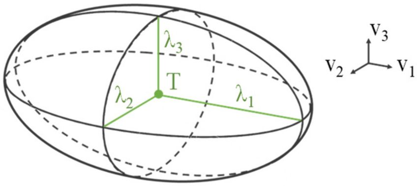
Metrology 2022, 2 250
This function is so parametrized by θ ◦ . In the same manner, similar formulas are
obtained for the other coordinates of the four measurement heads of the observation vector
λ. Besides, for the distances di :
√ 2
( di − ( x Hi ◦ − x T ◦ )2 +(y Hi ◦ −y T ◦ )2 +(z Hi ◦ −z T ◦ )2 )
1 −
2σdi 2
f di (di )= p e
2πσdi 2
(35)
( d i − d i ◦ )2
1 −
2σdi 2
= p e
2πσdi 2
The log-likelihood function can then be developed as follows since the variables of the
observation vector are statistically independent of each other [28]:
m m m
l (θ ◦ |λ) = ∑ ln f di (di ; θ ◦ ) + ∑ ln f xHi ( x Hi ; θ ◦ ) + ∑ ln f yHi (y Hi ; θ ◦ ) . . .
i =1 i =1 i =1
m
+ ∑ ln f zHi (z Hi ; θ◦ )
i =1 (36)
m m
= ∑ ln f di (di ; x T ◦ , y T ◦ , z T ◦ , x Hi ◦ , y Hi ◦ , z Hi ◦ ) + ∑ ln f xHi ( x Hi ; x Hi ◦ ) . . .
i =1 i =1
m m
+ ∑ ln f yHi (y Hi ; y Hi ◦) + f zHi (z Hi ; z Hi ◦ )
∑ ln
i =1 i =1
From this, the calculation of the FIM can be performed. After an onerous calculation,
not detailed in this paper, the three block matrices X, Y and Z are equal to [27,29]:
X = Md T × cov(d)−1 × Md
Y = Md T × cov(d)−1 × M H (37)
Z = M H T × cov(d)−1 × M H + cov( H )−1
with cov(d) defined in Formula (11) and:
h i
cov( H ) = diag σxH1 2 , σyH1 2 , σzH1 2 , . . . , σxH1 2 . (38)
x T ◦ − x H1 ◦ y T ◦ −y H1 ◦ z T ◦ −z H1 ◦
d1 d1 d1
.. .. ..
. . .
∂d
Md = = (39)
∂T ◦ .. .. ..
. . .
x T ◦ − x H4 ◦ y T ◦ −y H4 ◦ z T ◦ −z H4 ◦
d4 d4 d4
x T ◦ − x H1 ◦ y T ◦ −y H1 ◦ z T ◦ −z H1 ◦
d1 d1 d1
0 0
..
x T ◦ − x H2 ◦
∂d 0 0 0 d2 .
MH = ◦ = (40)
∂H .. .. ..
. . .
y T ◦ −y H4 ◦
x T ◦ − x H4 ◦ z T ◦ −z H4 ◦
0 0 d4 d4 d4
At the end, the CRLB of the target location corresponds to the upper left 3 × 3
submatrix of the inverse of the FIM. As previously, by proceeding to a singular value
decomposition of this matrix, the confidence ellipsoid of the target can be obtained.
4. Multilateration with Self-Calibration
4.1. Determination of the Targets and Head Positions
In a multilateration technique with self-calibration, the measurement heads are located
at unknown positions. However, by performing distance measurements for several target
positions, a system of equations with more observations than unknowns is created. Thus,Metrology 2022, 2 251
the coordinates of each target position, but also the coordinates of the measurement heads
can be determined.
The multilateration algorithm with self-calibration requires initial values sufficiently
accurate for the target and head positions [30]. For that purpose, in our system, the n
positions of the targets are determined with an accuracy around 1 mm from the measure-
ments of a single head, in the same way as a laser tracker. Indeed, each measurement head
also records its two orthogonal angles (horizontal and vertical), thanks to angle encoders
of around 400 µrad of resolution. Thus, in a cartesian system, the rough estimate of the
position of a target j is:
x j = di,j × sin ϕi cos θi , y j = di,j × sin ϕi sin θi , z j = di,j × cos ϕi (41)
with di,j the distances measured by the measurement head i (positive values), θ i and ϕi
the azimuth and elevation angles of this head (in radians, θ i between 0 and 2π and ϕi
between –π/2 and +π/2). This corresponds to the standard transformation from spherical
to Cartesian coordinates.
In practice, the results from several heads are combined to mitigates the errors. To this
end, a registration step based on Horn’s quaternion-based method is performed to express
the different results in a unique system of coordinates. This consists of finding rotation
matrices and translation vectors that best match one collection of target coordinates to
another in a least-squares sense. Once that is carried out, a fusion algorithm is applied [23].
Lastly, when the initial values of the target positions have been determined, the initial
values of the measurement head positions are calculated using the multilateration algorithm
presented in Section 2.
At this step, the heads and targets are referenced in a new system of coordinates where
one head defines the origin, a second one defines the x axis, and a last one defines the
xOy plane. An example is provided in Equation (43). This is an arbitrary choice to fix
the orientation of the coordinate system, but at the end, the positions of the heads and
of the targets could be transformed into any coordinate system, thanks to a translation
and rotations.
[ x1 , y1 , z1 ] = [ 0 , 0 , 0 ]
[ x2 , y2 , z2 ] = [ x2 , 0 , 0 ] (42)
[ x3 , y3 , z3 ] = [ x3 , y3 , 0]
The coordinates x2 , x3 , y3 and those of the other measurement heads must now be
refined from their initial values. To do this, the following cost function is minimized:
2 2
∑ di,j 2 − Hi − Tj Hi , di,j
cost f unction = (43)
i, j
where the unknown inputs are the coordinates of the heads, reduced by 6 since some
of them have been fixed to zero. For a given set of inputs Hi , the coordinates of the
target positions Tj are calculated from the measured distances by using the multilateration
algorithm presented in Section 2.
From a geometrical point of view, minimizing the cost function in Formula (43) is like
looking for the radical center of four spheres, i.e., minimization of the sum of the squares of
the power of the point Tj with respect to a sphere of center Hi and radius di,j [31].
In practice, a Levenberg–Marquardt method has been adopted to minimize the cost
function. It is an algorithm for solving the non-linear least-squares problems. Like the
Gauss–Newton method, it proceeds iteratively, and uses the Jacobian to define an error
correction vector. However, it has the advantage of offering a better stability against the
rank-deficiency of the Jacobian matrix [32].
When the cost function is minimized, and so the coordinates of the heads determined,
the uncertainties on these coordinates are determined. By this way, the problem is basically
the same as the one presented in Section 3: A multilateration system where the positions of
the heads and their uncertainties are known.Metrology 2022, 2 252
4.2. Uncertainty Assessment
For multilateration algorithm with self-calibration, the FIM (or CRLB) is not used to
analytically determine the uncertainties of the coordinates since it is rank deficient due
to the translational and rotational ambiguity in the self-calibration solution [33]. In other
words, the FIM is not invertible. To solve this problem, we propose in this paper our
own solution.
First, we impose constraints on the multilateration problem in Formula (43) to remove
the ambiguity. In our case, this consists of studying each measurement head separately: for
a given head, numbered k, the problem is simplified considering that the coordinates of
the heads Hi are known, error-free when i 6= k and noise corrupted only when i = k. An
approximation of the uncertainties of the coordinates of the heads can then be calculated
on the basis of the empirical study in [34], which presents a method to determine the
covariance matrix of parameters estimated by non-linear least-squares. To this end, it is
assumed that the distances between the different measurement heads and targets can be
written as a mathematical function f :
f θ = Hk , di,j , Hi = Hi − Tj di,j , Hi (44)
with the target positions Tj determined from the classical multilateration algorithm pre-
sented in Section 2 using the measured distances di,j and the coordinates [xHi , yHi , zHi ]
determined in Section 4.1.
The measured distances di,j are the response variables, while the positions of both
targets Tj and heads Hi (with i 6= k) are the predictor variables. The parameter to estimate
is here θ ◦ , the true but unknown coordinates of Hk . At the end, the measured distances di,j
can therefore be modelled as follows:
di,j = f θ ◦ , Tj , Hi + ei,j
(45)
with ei,j random errors between the measured distances and the true ones. These errors
are assumed independent and Gaussian distributed of mean equal to zero. According
to [34], the covariance matrix of the estimated coordinates θ can be approximated from the
Jacobian of f at the position θ = [xHk , yHk , zHk ].
−1
cov(θ = Hk ) = s2 × J ( Hk ) T J ( Hk ) (46)
where s is the estimated residual variance of f at position Hk :
m n
1
×∑ ∑
2
s2 = di,j − f ( Hk ) (47)
m × n − p i =1 j =1
with p is the length of vector θ, i.e., p = 3.
The Jacobian matrix of f at position Hk describes how small changes into the coordi-
nates of the head Hk will modify the distances derived from that position.
∂ f (θ ) ∂ f (θ ) ∂ f (θ )
J ( Hk ) = ∂x H ∂y H ∂z H (48)
k Hk k Hk k Hk
The calculation of the first-order partial derivatives of f (θ) appears particularly com-
plex. It is in fact numerically differentiated at the estimated value Hk , for instance using the
jacobianest function under Matlab® [35].
In the proposed approach, each measurement head is treated independently. This
approach is justified by the fact that if we consider in Formula (46) a function f of input
variables the coordinates of all the measurement heads, the obtained covariance matrix
would be rank-deficient with a rank equal to 3 × (m − 6).Metrology 2022, 2 253
As previously, from the covariance matrix of the estimated position θ, the confidence
ellipsoid of each measurement head can be determined. This is now a multilateration
problem with the uncertainties on both the distance measurements and the measurement
head positions as previously presented in Section 3. It is therefore easy to also determine
the uncertainties on the target positions.
Lastly, once the target positions and their uncertainties known, the uncertainties of the
coordinates of the heads (but not their value) are refined using the method in Section 3.2.
Section 5 compares this analytical approach for computing the uncertainties, and so
the confidence regions, from experimental results to Monte Carlo simulations.
4.3. Instrument Offsets
In the developed system, there are also instrument offsets to consider, one per mea-
surement head. They are additive constants, expressed in meters, that compensate from
delays in cables, electrical components and optical paths. Such corrections are required
to have an electro-optical origin that corresponds to the zero of the instrument, and so to
achieve absolute distance measurements between each measurement head and the targets.
di,j absolute = di,j + oi (49)
with oi the offset linked to the head Hi .
In practice, these offsets can be determined, thanks to additional measurements on a
small baseline composed of three pillars [36]: with the developed system, this calibration
step provides offsets with uncertainties of a few micrometers.
Alternatively, these additional unknown variables can also be determined simulta-
neously to the multilateration measurement with self-calibration. To this end, the cost
function in Formula (43) is modified as follows:
2 2
∑
2
cost f unction = di,j + oi − Hi − Tj Hi , di,j + oi (50)
i,j
Once the offsets have been determined by using one of the two above methods, the
measured distances are corrected. The offsets are assumed constant. As a consequence, the
offset calibration of the developed coordinate measurement system can be performed just
once. In practice, it is better to determine them occasionally because they can change with
time due to, for instance, a temperature dependency.
If we assume that the measured distances were corrected from the offsets after a first
calibration step: the offsets are known, but affected by an additive zero-mean Gaussian
noise of known standard deviation. Thus, we can perform multilateration measurements
with self-calibration as detailed in Section 4 by replacing the measured distances by the
absolute distances calculated in Formula (49). In that case, the uncertainties on the absolute
distances are calculated as follows:
2
σdi,j absolute = σdi,j 2 + σoi 2 (51)
In this paper, the uncertainty assessment of a multilateration measurement with a
self-calibration that includes the offsets has not been considered. In such a case, with
unknown offsets, it is like if the observations, i.e., the measured distances di,j , are corrupted
by non-zero mean errors: the random errors ei,j in Formula (45) include also the offset, they
do not have therefore a zero mean value. The method proposed in Section 4.2 and based on
the empirical study in [34] is simply not valid.Metrology 2022, 2 254
5. Experimental Results versus Monte-Carlo Simulations for Multilateration with
Self-Calibration
5.1. Experimental Results
To validate the approach developed in Section 4 that provides the confidence ellipsoids
of the target and measurement head positions, three different experimental measurements
have been performed:
• The first case is a small volume of one cubic meter using a corner cube as target in 14
different positions.
• The second case is a large volume with distances up to 11.5 m and a corner cube in 14
different positions.
• The third case is a small volume of one cubic meter using a glass sphere of index n = 2
as target in 16 different positions.
Figure 4 depicts the layouts of the 4 measurement heads (identified by letters from
A to D corresponding to heads Hi , with i from 1 to 4) and of the different target positions
for these three experimental cases. The arrangements of the heads were always close to a
regular tetrahedron in order to optimize the uncertainties (see Figure 3a), and the targets
were preferably placed inside the volume formed by the heads, with the exception of
specific cases for testing longer distances.
Figure 4. Top view of the layouts of the 4 measurement heads and of the targets for the three
experimental measurements that were carried out (a–c). In the two first cases (a,b), a corner cube is
used as target, while in the last case (c), a glass sphere is used as target.
The uncertainty on the measured distances (at k = 1) has been assessed at 4.7 µm when
the target is a corner cube [2] and at 4.3 µm when it is a glass sphere of index n = 2 [3].
These values include the contribution of the target uncertainty. When the target is a corner
cube, the target can be oriented in any direction by means of a gimbal mechanism. Like any
mechanical system, not perfectly machined and assembled, this gimbal mechanism induces
errors on the geometric distances. These errors have been characterized, then minimized
by adjusting the position of the corner cube into the gimbal mechanism. In addition, some
systematic errors are corrected. At the end, they represent the main contribution to the
uncertainty of the distance measurements with a value of 3.9 µm (k = 1, zero-mean Gaussian
distributed [2]). When the target is a sphere visible from almost any angle, it does not
require such a mechanism. In this case, the main contribution to the distance uncertainty
comes from the random noise of 2.1 µm observed on the distance measurements. In fact,
the random noise is lower when a corner cube is used and is equal to 0.8 µm. The bad
reflectivity of the spheres and the beam deflection they induce increase the random noise.
However, the uncertainty may be a little bit higher in practice due to the determination ofMetrology 2022, 2 255
the atmospheric parameters, especially in the large volume where a vertical temperature
gradient of 1 ◦ C was observed.
The multilateration algorithm with self-calibration described in Section 4.1 has been
applied to the three experimental measurements to obtain the positions of both targets and
measurement heads. However, it must be emphasized that in all these cases, the instrument
offsets have been determined simultaneously to the multilateration process, which is the
critical case where the uncertainty assessment has not been studied. The algorithm has
always perfectly converged: the standard deviations on the difference between the distances
measured by our absolute distance meter, and those deduced from the positions provided
by the multilateration algorithm were always lower than 4 µm.
Then, from the uncertainty assessment described in Section 4.2, all the determined
positions k (both heads and targets) have been characterized by a covariance matrix and
an associated confidence ellipsoid. We have operated ignoring the instrument offsets, as if
they had no impact. This approach should be seen as an approximation in the absence of
any more reliable solution. The comparisons presented subsequently will assess the impact
of this choice.
The uncertainty, expressed as a single-number indicator, has been calculated as follows:
q
σ ( posk ) = Trace(cov( posk )) (52)
To validate the experimental results, reference measurements are required. To address
this issue, some distances between different target positions have been measured in a direct
way by the absolute distance meter (it means without multilateration) and compared to the
same distances when calculated from the target positions provided by the multilateration
algorithm. For the small volumes, these points correspond to a triplet of aligned target
positions mounted on a same breadboard, breadboard which has been displaced several
times into the volume. For the large volume, these points correspond to a couple of
target positions mounted on a same breadboard, and to three aligned pillars. Table 1
summarized the results, with the column d1 for the interpoint distances calculated from the
target positions (multilateration algorithm) and the column d3 for the interpoint distances
measured in a direct way.
An interpoint distance measured in a direct way is the difference between two dis-
tance measurements performed by the absolute distance meter when it is positioned in the
alignment of two target positions. These measurements were carried out after the multilat-
eration measurements, the target was so removed and mounted again in their holders, i.e.,
tribraches. The results were therefore limited by the centring repeatability of the tribraches
equal to 5 µm [37]. At the end, the uncertainty σ3 on the interpoint distance was assessed
to 7.1 µm, which corresponds the combined uncertainty of two distance measurements.
The uncertainties σ1 on the distances d1 have also been calculated as the combined
uncertainty of two positions. Let Ta and Tb be these two target positions. Uncertainty of Ta
with respect to Tb , noted σa , can be deducted from its confidence ellipsoid: it is equal to
the distance between its ellipsoid centre (of coordinates Ta ) and the point of the ellipsoid
in the direction of Tb ; and inversely for uncertainty of Tb with respect to Ta . If the used
confidence ellipsoids (at 68%) correspond to trivariate error distributions, a 1.88 scaling
factor has to be applied to recover a one-dimensional error distribution, as reminded in
Section 2.2. Uncertainty σ1 can then be written in the following form:
1
q
σ1 (k Ta − Tb k) = × σa 2 + σb 2 (53)
1.88Metrology 2022, 2 256
Table 1. Comparison of the interpoint distances.
Monte-Carlo
Measured Experimental Results Direct Measurements
Case Simulations
Distance
d1 (mm) σ 1 (µm) d2 (mm) σ 2 (µm) d3 (mm) σ 3 (µm)
kT1 –T2 k 150.030 6.5 150.030 6.4 150.022
triplet 1 kT2 –T3 k 174.628 7.2 174.628 7.2 174.615
kT1 –T3 k 324.657 6.9 324.657 6.9 324.636
kT6 –T7 k 150.022 6.1 150.022 7.0 150.022
small volume,
corner cube triplet 2 kT7 –T8 k 174.637 6.7 174.637 6.7 174.615
kT6 –T8 k 324.657 6.3 324.658 6.8 324.636
kT12 –T13 k 150.018 5.9 150.018 5.7 150.022
triplet 3 kT13 –T14 k 174.609 6.0 174.608 5.9 174.615
kT12 –T14 k 324.625 6.0 324.624 5.9 324.636 7.1
kT1 –T2 k 324.088 5.6 324.088 6.4 324.071
3 couples kT3 –T4 k 324.082 4.6 324.081 5.0 324.071
large volume, kT5 –T6 k 324.067 5.0 324.067 5.5 324.071
corner cube kT12 –T13 k 2232.049 4.3 2232.049 4.8 2232.037
3 pillars kT13 –T14 k 6700.461 3.8 6700.461 5.1 6700.471
kT12 –T14 k 8932.505 4.1 8932.506 5.3 8932.509
kT2 –T3 k 150.090 3.7 150.091 4.0 150.096
triplet 1 kT3 –T4 k 174.410 3.6 174.411 4.0 174.410
kT2 –T4 k 324.498 3.7 324.500 4.1 324.506
kT5 –T6 k 150.087 5.4 150.087 5.6 150.096
small volume,
glass sphere triplet 2 kT6 –T7 k 174.427 5.2 174.424 5.9 174.410
kT5 –T7 k 324.512 5.3 324.509 5.8 324.506
kT9 –T10 k 150.116 7.5 150.114 7.9 150.096
triplet 3 kT10 –T11 k 174.415 7.0 174.419 7.7 174.410
kT9 –T11 k 324.529 7.2 324.531 7.6 324.506
5.2. Monte-Carlo Simulations
In parallel, Monte-Carlo simulations have been performed. Figure 5 describes how
they were constructed.
First, for each geometric arrangement depicted in Figure 4, we calculate the true
distances between the measurement heads and the target positions assuming all positions
perfectly known. Then, we simulate the measured distances adding a zero-mean Gaussian
noise of standard deviation 4.7 µm or 4.3 µm according to the used target, i.e., a corner cube
or a glass sphere. We also generate the initial values needed to launch our multilateration
algorithm with self-calibration: a zero-mean Gaussian noise of standard deviation 1 mm
is thus added to simulate the results of a single head used as a laser tracker. Lastly, the
multilateration algorithm is applied and the resulting positions are recorded. It has to be
noted that the Monte-Carlo simulations have considered a system that has no instrument
offset. The simulated measured distances are therefore not affected by an additional noise
due to the instrument offsets. This corresponds to the ideal case described in Section 4.Metrology 2022, 2 257
Figure 5. The Monte-Carlo diagram.
The Monte-Carlo simulations were made under Matlab® , and for each simulation,
the random sampling of the measured distances and of the initial measurement head
coordinates was repeated 500 times. The simulated outputs are positions Hi and Tj , which
are compared with the true ones Hi ◦ and Tj ◦ . The true positions are here the results of the
experimental measurements. In order to know how well the analytical calculation of the
uncertainties fits the Monte-Carlo simulations, a definition of the Monte-Carlo uncertainties
has to be provided. It is equal to the mean radial spherical error (MRSE), a single-number
indicator used in the global navigation satellite system (GNSS) world [38]:
q
2
MRSE( posk ) = σ (∆ x ( posk ))2 + σ ∆y ( posk ) + σ(∆z ( posk ))2 (54)
with σ the function that returns the standard deviation and ∆x , ∆y and ∆z the vectors of
the differences between the true position k and the positions observed after a Monte-Carlo
simulation along each of the three axes. According to [38], the MRSE contains about 61%
probability, a confidence region close enough to the one defined in Formula (52) to perform
a comparison.
As explained in Section 4.1, the measurement heads are set arbitrarily in a system of
coordinates where the head A defines the origin, the head B defines the x axis, and the
head C defines the xOy plane. Thus, due to the algorithm design, xA , yA , zA , yB , zB , and zC
are always equal to zero and any error cannot be noticed on these coordinates. However,
forcing certain coordinates values may result in excessive errors on others. Therefore,
before calculating the errors, a registration step based on Horn’s quaternion-based method
has been added: this consists of finding a translational vector and a rotational matrix
that best match the positions of the heads and targets obtained by multilateration to their
true coordinates in a weighted least-squares sense. The applied weights are here the
inverse of the square analytical position uncertainties. It has to noted that the uncertainty
calculation in Section 4.2 also considered uncertainties for each head so as not to obtain
zero uncertainties on some heads and excessive uncertainties on others.
As shown in Figure 5, the MRSE have been compared to the uncertainties calculated
analytically from the experimental data, σ(posk ), as described in Section 4.2.
As previously, a comparison of interpoint distances instead of positions is still relevant.
Thus, to complete Table 1, the average value over 500 iterations of some interpoint distances
have been reported in the column d2 as well as the corresponding standard deviation σ2 .
5.3. Results
In Figure 6, the MRSE computed from the Monte-Carlo simulations has been compared
to the analytical uncertainties calculated from a set of data randomly generated. TheMetrology 2022, 2 258
discrepancy between the two approaches is low for the target positions, with errors of few
micrometers only. Nevertheless, the results appear less consistent for the measurement
heads. In addition, it should be recalled that the analytical uncertainties in Formula (52)
represent a confidence region of 68% while MRSE in Formula (54) represents a confidence
region around 61%. The MRSE should be lower than the analytical results, which is not
necessarily the case.
Figure 6. Comparison between the Monte-Carlo simulations and the analytical calculation of the
uncertainties for the three experimental measurements that were carried out (a–c). The number of the
positions is indicated when the obtained uncertainties are high.
MRSE and σ(posk ) are usefull to, respectively, quantify and anticipated the uncertain-
ties of a position using single numbers. However, they do not describe the geometry of the
errors. Consequently, the confidence ellipsoids have been directly compared to the results
of the Monte-Carlo simulations as shown in Figure 7 with the second configuration, i.e., the
large volume, and when the corner cube is located in position 14. This case corresponds
to the highest observed uncertainty with a RMSE around 40 µm. In Figure 7, the 500
positions obtained from the Monte-Carlo simulation have been projected on the plane of
the confidence ellipse of eigenvectors v1 and v2, then on the plane of the confidence ellipse
of eigenvectors v2 and v3. These orthonormal vectors are the eigenvectors of the confidence
ellipsoid (at 68%) of the position 14. The red dot corresponds to the true position, while the
other dots correspond to the results of the Monte-Carlo simulation, with in green the points
inside the ellipse and in blue those outside the ellipse. In theory, the probability that the
projections of the three-dimensional points from the simulation on these planes lie within
the confidence ellipses is equal to 82.9% [24]. The simulation results are, therefore, very
close to the expected values with percentages of 84% for the v1–v2 plane and 78% for the
v2–v3 plane. In addition, the shape of the confidence ellipsoid is a good approximation of
the shape of the true contour. Figures 6 and 7 validate, therefore, the analytical calculation
of the uncertainties.
Figure 7. Case 2—multilateration in a large volume when the target, a corner cube, is in position 14:
positions obtained from the Monte-Carlo simulation versus confidence ellipsoid at 68%.Metrology 2022, 2 259
As shown in Figure 8, the results of the Monte-Carlo simulations were also depicted
for the case 3, when a glass sphere is used. For this position, numbered 14, percentages of
80% and 75% were obtained for the v1–v2 and v2–v3 planes, respectively.
Figure 8. Case 3—multilateration in a small volume when the target, a sphere, is in position 14:
positions obtained from the Monte-Carlo simulation versus confidence ellipsoid at 68%.
At the end, with our system composed of four measurement heads, and for the
geometrical arrangements depicted in Figure 4, we typically obtain uncertainties on the
positions of both heads and targets between 6 µm and 10 µm for a small volume of one
cubic meter and between 10 µm and 22 µm for the large volume. The positions outside the
volume formed by the heads have higher uncertainties, for instance the target positions 5
and 10 in case 1, 14 in case 2, 10, 15 and 16 in case 3. However, from the results presented
in Section 2.3 for optimal arrangements of the measurement heads, we would expect in
Figure 6 uncertainties always higher than 1.5 × σd ~7 µm (value depicted with an orange
vertical line). For instance, in the case 3, the analytical calculation of the uncertainties of the
target 14 equals to 6.2 µm, when the corresponding MRSE equals to 6.6 µm. This analytical
result is therefore slightly undervalued (by 6%), which is confirmed in Figure 8.
Concerning the interpoint distances, the process to determine their value is recalled in
Figure 9 while the results are presented in Table 1. First, the Monte-Carlo simulations, built
from data of the experimental measurements, give the same results as the experimental
measurements. Then, it has been verified that the experimental results are consistent with
the direct distance measurements. Thus, in Figure 10, the distances d1 and d3 have been
plotted, relatively to the distances d3 considered here as reference values, with uncertainty
bars corresponding to the uncertainties σ1 and σ3 , respectively. These uncertainty bars
are consistent between them for 16 interpoint distances over 24, i.e., 67% of the points lie
within one standard deviation (for 68% expected).
As explained previously, in the experimental measurements, four instrument offsets
have been determined by the multilateration algorithm with self-calibration in addition to
the coordinates of the measurement heads and targets. On the contrary, in the Monte-Carlo
simulations, there were no instrument offsets. Nevertheless, in both cases, the uncertainties
have been evaluated in the same manner by considering there were no instrument offset.
The consideration of the offsets for the experimental measurements would surely
increase the uncertainties of all the positions, and so σ1 . However, in the absence of a math-
ematical method to determine these uncertainties, the results achieved in Figure 10 show a
good agreement between the experimental measurements and the direct measurements.Metrology 2022, 2 260
Figure 9. Description of the determination of d1 , d2 and d3 and of their associated uncertainties.
Figure 10. Comparison of the experimental results d1 with the direct distance measurements d3 for the
three experimental measurements that were carried out (a–c), with uncertainty bars corresponding to
confidence intervals of 68% (k = 1).
6. Conclusions
Our objective was to assess with a consistent metrological approach the uncertainties
of target positions obtained with our coordinate measurement system. For this purpose,
the uncertainty contribution of the data processing has been studied: we have provided an
analytical solution for the uncertainty assessment of both targets and heads under different
multilateration scenarios.
The original point here was the multilateration algorithm with self-calibration. For this
case, we have proposed our own method to assess the uncertainties. First, an approximation
of the uncertainties of the coordinates of the heads was calculated from the estimate of
Jacobian matrices. The problem was then addressed as a multilateration algorithm with
uncertainties on both the distance measurements and the measurement head positions. It
was therefore easy to determine the uncertainties of the target positions from the Fisher
information matrix (FIM). Lastly, the uncertainties of the coordinates of the heads were
refined from the target positions using again the FIM.
This new approach has then been validated, thanks to comparisons between experi-
mental measurements made with our system and Monte-Carlo simulations. It has been
demonstrated that the analytical solution for uncertainty assessment provides results very
close to the Monte-Carlo simulations, with differences of few micrometres only. Moreover,
the confidence ellipsoids provided by the analytical approach describe well the geometry
of the errors. It is, therefore, possible to determine the uncertainties in different directions.
At the end, the accuracy that can be achieved with the developed system, when the
arrangement of the heads is close to a regular tetrahedron, is typically between 6 µm andYou can also read